Dielectric function of the semiconductor hole liquid:
Full frequency and wave vector dependence

Abstract

We study the dielectric function of the homogeneous semiconductor hole liquid of $p$-doped bulk III-V zinc-blende semiconductors within random phase approximation. The single-particle physics of the hole system is modeled by Luttinger’s four-band Hamiltonian in its spherical approximation. Regarding the Coulomb-interacting hole liquid, the full dependence of the zero-temperature dielectric function on wave vector and frequency is explored. The imaginary part of the dielectric function is analytically obtained in terms of complicated but fully elementary expressions, while in the result for the real part nonelementary one-dimensional integrations remain to be performed. The correctness of these two independent calculations is checked via Kramers-Kronig relations.

The mass difference between heavy and light holes, along with variations in the background dielectric constant, leads to dramatic alternations in the plasmon excitation pattern, and generically, two plasmon branches can be identified. These findings are the result of the evaluation of the full dielectric function and are not accessible via a high-frequency expansion. In the static limit a beating of Friedel oscillations between the Fermi wave numbers of heavy and light holes occurs.

I Introduction

The interacting electron gas, combined with a homogeneous neutralizing background, is one of the paradigmatic systems of many-body physics Giuliani05 ; Mahan00 ; Bruus04 . Albeit the result of drastic approximations, its predictions provide a good description of important properties of three-dimensional bulk metals and, in the regime of lower carrier densities, $n$-doped semiconductors where the electrons reside in the s-type conduction band.

On the other hand, in a $p$-doped zinc-blende III-V semiconductor such as GaAs, the defect electrons or holes occupy the p-type valence band whose more complex band structure can be expected to significantly modify the electronic properties. Moreover, the most intensively studied ferromagnetic semiconductors such as Mn-doped GaAs are in fact $p$-doped with the holes playing the key role in the occurrence of carrier-mediated ferromagnetism among the localized Mn magnetic moments Jungwirth06 . Thus, such $p$-doped bulk semiconductor systems lie at the very heart of the still growing field of spintronics Fabian07 , and therefore it appears highly desirable to gain a deeper understanding of their many-body physics.

Ab-initio-type approaches to the description of ferromagnetic semiconductors constitute an important subfield of this endeavor, and there is a lively discussion on strengths and weaknesses of the pertaining concepts and numerical techniquesSato10 . In the present paper we will follow a somewhat different route by developing an analytical theory of the most prominent class of host materials given by $p$-doped bulk III-V zinc-blende systems such as GaAs. Specifically, we investigate the dielectric function of the interacting hole liquid within random phase approximation (RPA)Giuliani05 ; Mahan00 ; Bruus04 where the non-interacting hole system in the valence band is described by Luttinger’s Hamiltonian in the spherical approximationLuttinger56 . We evaluate the zero-temperature dielectric function in the entire range of wave vectors and frequencies building upon a recent study where the problem was analyzed in the static limit, and in the case of large frequenciesSchliemann10 . Another previous work investigated, among other issues, properties of Hartree-Fock solutions of the two-component carrier system consisting of heavy and light holesSchliemann06 . Moreover, very recently Kyrychenko and Ullrich have put forward a study of holes in magnetically doped III-V systems Kyrychenko09 by modeling the band structure by an $8\times 8$ $\vec{k}\cdot\vec{p}$ Hamiltonian (similar as in the present work) while disorder effects and interaction among the carriers are treated by a combination of equations-of-motion techniques and time-dependent density functional theory Kyrychenko09 ; Kyrychenko11 . Further below we will compare our fairly analytical results with the ones of Ref. Kyrychenko11 which rely heavier on numerical evaluations.

Finally we mention a series of related recent studies of the dielectric properties of two-dimensional fermionic systems (instead of three-dimensional bulk semiconductors) whose single-particle states carry a non-trivial spinor structure. These include $n$-doped quantum wells with spin-orbit coupling Pletyukhov06 ; Badalyan09 ; Agarwal11 ; Chesi11 and two-dimensional hole systems Kernreiter10 . Other recent investigations have dealt with planar graphene sheets where an effective spin is incorporated by the sublattice degree of freedomWunsch06 ; Stauber10 ; Pyatkovskiy09 .

The plan of the paper is as follows. In section II we give an overview on elementary properties of the single-particle Hamiltonian describing the band structure around the $\Gamma$-point, and on the many-body formalism leading to the RPA result for the dielectric function. In Section III we present explicit analytical expressions for the free polarizability; the corresponding derivations are deferred to the appendices. Section IV discusses physical properties of the dielectric function and its full dependence on wave vector and frequency. Special attention is paid to the static limit, and to the limit of large frequencies. We close with conclusions and an outlook in section V.

II Preliminaries: Hamiltonian, eigensystem, and many-body formalism

Luttinger’s Hamiltonian describing heavy and light hole states around the $\Gamma$-point in III-V zinc-blende semiconductors reads in its spherical approximationLuttinger56 ,

$${\cal H}=\frac{1}{2m_{0}}\left(\left(\gamma_{1}+\frac{5}{2}\gamma_{2}\right)\vec{p}^{2}-2\gamma_{2}\left(\vec{p}\cdot\vec{S}\right)^{2}\right)\,.$$ (1)

Here $m_{0}$ is the bare electron mass, $\vec{p}$ is the hole lattice momentum, and $\vec{S}$ are spin-$3/2$-operators, resulting from adding the $l=1$ orbital angular momentum to the $s=1/2$ electron spin. The dimensionless Luttinger parameters $\gamma_{1}$ and $\gamma_{2}$ describe the valence band of the specific material with effects of spin-orbit coupling being included in $\gamma_{2}$. We note that , while the present work is mostly motivated by III-V semiconductors, the above model for the $\Gamma_{8}$ valence band also applies to other systems with zinc-blende or diamond structure including elemental semiconductors like Si and Ge, but also zero-gap semiconductors such as HgSe and HgTe.

The above Hamiltonian is rotationally invariant and commutes with the helicity operator $\lambda=(\vec{k}\cdot\vec{S})/k$, where $\vec{k}=\vec{p}/\hbar$ is the hole wave vector. The heavy (light) holes correspond to $\lambda=\pm 3/2$ ($\lambda=\pm 1/2$) with the energy dispersions

$$\varepsilon_{h/l}(\vec{k})=\frac{\hbar^{2}k^{2}}{2m_{h/l}}$$ (2)

and heavy ($h$) and light ($l$) hole masses $m_{h/l}=m_{0}/(\gamma_{1}\mp 2\gamma_{2})$. The corresponding eigenstates are given by

$$\langle\vec{r}|\vec{k},\lambda\rangle=\frac{e^{i\vec{k}\vec{r}}}{\sqrt{V}}|\chi_{\lambda}(\vec{k})\rangle\,,$$ (3)

where $V$ is the volume of the system. Using the conventional basis of eigenstates of $S^{z}$ and introducing polar coordinates $\vec{k}=k(\cos\varphi\sin\vartheta,\sin\varphi\sin\vartheta,\cos\vartheta)$ , the eigenspinors $|\chi_{\lambda}(\vec{k})\rangle$ of the helicity operator read explicitly Schliemann06

$$|\chi_{\frac{3}{2}}(\vec{k})\rangle = \left(\begin{array}[]{c}\cos^{3}\frac{\vartheta}{2}e^{-\frac{3i}{2}\varphi}\\ \sqrt{3}\cos^{2}\frac{\vartheta}{2}\sin\frac{\vartheta}{2}e^{-\frac{i}{2}\varphi}\\ \sqrt{3}\cos\frac{\vartheta}{2}\sin^{2}\frac{\vartheta}{2}e^{+\frac{i}{2}\varphi}\\ \sin^{3}\frac{\vartheta}{2}e^{+\frac{3i}{2}\varphi}\end{array}\right)$$ (8)

$$|\chi_{\frac{1}{2}}(\vec{k})\rangle = \left(\begin{array}[]{c}-\sqrt{3}\cos^{2}\frac{\vartheta}{2}\sin\frac{\vartheta}{2}e^{-\frac{3i}{2}\varphi}\\ \cos\frac{\vartheta}{2}\left(\cos^{2}\frac{\vartheta}{2}-2\sin^{2}\frac{\vartheta}{2}\right)e^{-\frac{i}{2}\varphi}\\ \sin\frac{\vartheta}{2}\left(2\cos^{2}\frac{\vartheta}{2}-\sin^{2}\frac{\vartheta}{2}\right)e^{+\frac{i}{2}\varphi}\\ \sqrt{3}\cos\frac{\vartheta}{2}\sin^{2}\frac{\vartheta}{2}e^{+\frac{3i}{2}\varphi}\end{array}\right)$$ (13)

and the remaining eigenspinors $|\chi_{-3/2}(\vec{k})\rangle$, $|\chi_{-1/2}(\vec{k})\rangle$ can be obtained from the above ones by spatial inversion $\vartheta\mapsto\pi-\vartheta$, $\varphi\mapsto\varphi+\pi$. In what follows, mutual overlaps squared Schliemann06 between spinors will be of key importance,

$$|\langle\chi_{\frac{3}{2}}(\vec{k}_{1})|\chi_{\frac{3}{2}}(\vec{k}_{2})\rangle|^{2} = \left(\frac{1}{2}\left(1+\frac{\vec{k}_{1}\vec{k}_{2}}{k_{1}k_{2}}\right)\right)^{3}$$ (14)

$$|\langle\chi_{\frac{1}{2}}(\vec{k}_{1})|\chi_{\frac{1}{2}}(\vec{k}_{2})\rangle|^{2} = \frac{1}{8}\left(1+\frac{\vec{k}_{1}\vec{k}_{2}}{k_{1}k_{2}}\right)\left(3\frac{\vec{k}_{1}\vec{k}_{2}}{k_{1}k_{2}}-1\right)^{2}$$ (15)

$$|\langle\chi_{\frac{3}{2}}(\vec{k}_{1})|\chi_{\frac{1}{2}}(\vec{k}_{2})\rangle|^{2} = \frac{3}{8}\left(1+\frac{\vec{k}_{1}\vec{k}_{2}}{k_{1}k_{2}}\right)^{2}\left(1-\frac{\vec{k}_{1}\vec{k}_{2}}{k_{1}k_{2}}\right)$$ (16)

Combining the above single-particle Hamiltonian with Coulomb repulsion among holes and a neutralizing background, the dielectric function within RPA at wave vector $\vec{q}$ and frequency $\omega$ is given byGiuliani05 ; Mahan00 ; Bruus04

$$\varepsilon^{RPA}(\vec{q},\omega)=1-V(\vec{q})\chi_{0}(\vec{q},\omega)\,.$$ (17)

Here $V(\vec{q})$ is the Fourier transform of the interaction potential, and the free polarizability reads

$$\chi_{0}(\vec{q},\omega) = \frac{1}{(2\pi)^{3}}\sum_{\lambda_{1},\lambda_{2}}\int d^{3}k\Biggl{[}\left|\langle\chi_{\lambda_{1}}(\vec{k})|\chi_{\lambda_{2}}(\vec{k}+\vec{q})\rangle\right|^{2}$$ (18)

$$\cdot\frac{f(\vec{k},\lambda_{1})-f(\vec{k}+\vec{q},\lambda_{2})}{\hbar\omega+i0-\left(\varepsilon_{\lambda_{2}}(\vec{k}+\vec{q})-\varepsilon_{\lambda_{1}}(\vec{k})\right)}\Biggr{]}$$

with $f(\vec{k},\lambda)$ being Fermi functions. In what follows we will concentrate on the case of zero temperature and Coulomb repulsion, $V(\vec{q})=e^{2}/(\varepsilon_{r}\varepsilon_{0}q^{2})$ where $\varepsilon_{r}$ is a background dielectric constant taking into account screening by deeper bands.

III The free polarizability

We now present our analytical results for the real and imaginary part of the free polarizability. Details of the derivations are can be found in appendices A.1 and A.2. A discussion of the physical properties of the corresponding dielectric function follows further below in section IV. Defining

$$\chi_{hh}(\vec{q},\omega)=\frac{1}{(2\pi)^{3}}\int_{k\leq k_{h}}d^{3}k\left(\frac{1}{2}+\frac{3}{2}\frac{\left(\vec{k}\cdot(\vec{k}+\vec{q})\right)^{2}}{k^{2}(\vec{k}+\vec{q})^{2}}\right)$$

$$\qquad\qquad\Biggl{[}\frac{1}{\hbar\left(\omega+i0\right)-\left(\varepsilon_{h}(\vec{k}+\vec{q})-\varepsilon_{h}(\vec{k})\right)}$$

$$\qquad\qquad-\frac{1}{\hbar\left(\omega+i0\right)+\left(\varepsilon_{h}(\vec{k}+\vec{q})-\varepsilon_{h}(\vec{k})\right)}\Biggr{]}\,,$$ (19)

$$\chi_{hl}(\vec{q},\omega)=\frac{1}{(2\pi)^{3}}\int_{k\leq k_{h}}d^{3}k\left(\frac{3}{2}-\frac{3}{2}\frac{\left(\vec{k}\cdot(\vec{k}+\vec{q})\right)^{2}}{k^{2}(\vec{k}+\vec{q})^{2}}\right)$$

$$\qquad\qquad\Biggl{[}\frac{1}{\hbar\left(\omega+i0\right)-\left(\varepsilon_{l}(\vec{k}+\vec{q})-\varepsilon_{h}(\vec{k})\right)}$$

$$\qquad\qquad-\frac{1}{\hbar\left(\omega+i0\right)+\left(\varepsilon_{l}(\vec{k}+\vec{q})-\varepsilon_{h}(\vec{k})\right)}\Biggr{]}\,,$$ (20)

one can formulate the polarizability (18) as follows,

$$\chi_{0}(\vec{q},\omega)=\sum_{\alpha,\beta\in\{h,l\}}\chi_{\alpha\beta}(\vec{q},\omega)\,,$$ (21)

where the remaining quantities $\chi_{ll}(\vec{q},\omega)$ and $\chi_{lh}(\vec{q},\omega)$ are given by (19) and (20) via the replacement $h\leftrightarrow l$, and $k_{h}$ ($k_{l}$) is the Fermi wave number for heavy (light) holes corresponding to the common Fermi energy $\varepsilon_{f}$.notechi Introducing the obvious decomposition $\chi_{\alpha\beta}(\vec{q},\omega)=R_{\alpha\beta}(\vec{q},\omega)+iI_{\alpha\beta}(\vec{q},\omega)$ with real functions $R_{\alpha\beta}(\vec{q},\omega)$, $I_{\alpha\beta}(\vec{q},\omega)$ ($\alpha,\beta\in\{h,l\}$), we will now analyze the real and imaginary part of the free polarizability of the hole gas. The respective expressions to be presented below are the result of independent calculations and perfectly fulfil Kramers-Kronig relationsGiuliani05 ; Mahan00 ; Bruus04 .

III.1 The real part of the free polarizability

Following the steps detailed in appendix A.1 the real part of the free polarizability can be obtained as

$$R_{hh}(\vec{q},\omega)+R_{hl}(\vec{q},\omega)=\frac{-m_{h}}{(2\pi\hbar)^{2}}\Biggl{[}2k_{h}+\frac{q}{4}\frac{1}{(\varepsilon_{h}(q))^{2}}\Biggl{(}\left(4\varepsilon_{f}\varepsilon_{h}(q)-\left(\varepsilon_{h}(q)+\hbar\omega\right)^{2}\right)\ln\left|\frac{\varepsilon_{h}(q)+\hbar\omega+\hbar^{2}qk_{h}/m_{h}}{\varepsilon_{h}(q)+\hbar\omega-\hbar^{2}qk_{h}/m_{h}}\right|$$

$$\qquad\qquad\qquad\qquad\qquad\qquad\qquad\qquad\qquad\qquad+\left(4\varepsilon_{f}\varepsilon_{h}(q)-\left(\varepsilon_{h}(q)-\hbar\omega\right)^{2}\right)\ln\left|\frac{\varepsilon_{h}(q)-\hbar\omega+\hbar^{2}qk_{h}/m_{h}}{\varepsilon_{h}(q)-\hbar\omega-\hbar^{2}qk_{h}/m_{h}}\right|\Biggr{)}\Biggr{]}$$

$$\qquad\qquad\qquad-\frac{3}{(2\pi\hbar)^{2}}\left(m_{h}-m_{l}\right)k_{h}$$

$$\qquad\qquad\qquad+\frac{3}{(2\pi\hbar)^{2}}\frac{m_{h}q}{32}\left(1-\frac{m_{h}}{m_{l}}\right)^{2}\left[\int_{0}^{2k_{h}/q}dyy\ln\left|\frac{1-\hbar\omega/\varepsilon_{l}(q)+y+(1-m_{l}/m_{h})y^{2}/4}{1-\hbar\omega/\varepsilon_{l}(q)-y+(1-m_{l}/m_{h})y^{2}/4}\right|+\left(\omega\mapsto-\omega\right)\right]$$

$$\qquad\qquad\qquad+\frac{3}{(2\pi\hbar)^{2}}\frac{m_{h}q}{8}\Biggl{[}\frac{\varepsilon_{h}(q)}{\hbar\omega}\left(1+\frac{\hbar\omega}{\varepsilon_{h}(q)}\right)^{2}{\cal P}\int_{0}^{2k_{h}/q}dy\frac{y}{y^{2}+4\hbar\omega/\varepsilon_{h}(q)}\Biggl{(}\ln\left|\frac{1-\hbar\omega/\varepsilon_{h}(q)+y}{1-\hbar\omega/\varepsilon_{h}(q)-y}\right|$$

$$\qquad\qquad\qquad\qquad\qquad\qquad\qquad\qquad\qquad\qquad-\ln\left|\frac{1-\hbar\omega/\varepsilon_{l}(q)+y+(1-m_{l}/m_{h})y^{2}/4}{1-\hbar\omega/\varepsilon_{l}(q)-y+(1-m_{l}/m_{h})y^{2}/4}\right|\Biggr{)}+\left(\omega\mapsto-\omega\right)\Biggr{]}$$

$$\qquad\qquad\qquad-\frac{3}{(2\pi\hbar)^{2}}\frac{m_{h}q}{8}\left[\frac{\varepsilon_{h}(q)}{\hbar\omega}\left(1-\frac{\hbar\omega}{\varepsilon_{h}(q)}\right)^{2}\int_{0}^{2k_{h}/q}dy\frac{1}{y}\ln\left|\frac{1-\hbar\omega/\varepsilon_{h}(q)+y}{1-\hbar\omega/\varepsilon_{h}(q)-y}\right|+\left(\omega\mapsto-\omega\right)\right]$$

$$\quad+\frac{3}{(2\pi\hbar)^{2}}\frac{m_{h}q}{8}\left[\frac{\varepsilon_{h}(q)}{\hbar\omega}\left(1-\frac{\hbar\omega}{\varepsilon_{l}(q)}\right)^{2}\int_{0}^{2k_{h}/q}dy\frac{1}{y}\ln\left|\frac{1-\hbar\omega/\varepsilon_{l}(q)+y+(1-m_{l}/m_{h})y^{2}/4}{1-\hbar\omega/\varepsilon_{l}(q)-y+(1-m_{l}/m_{h})y^{2}/4}\right|+\left(\omega\mapsto-\omega\right)\right]\,,$$ (22)

where $(\omega\mapsto-\omega)$ denotes terms with the sign of the frequency changed compared to the preceding expression, and the remaining contribution $R_{ll}(\vec{q},\omega)+R_{lh}(\vec{q},\omega)$ follows via $h\leftrightarrow l$. In the limit $m_{h}=m_{l}$ the first two lines in Eq. (22) express the result for the standard textbook case of a fermion gas without spin-orbit coupling Giuliani05 ; Mahan00 ; Bruus04 , while all other terms vanish in this limit and represent corrections arising from $m_{h}\neq m_{l}$. The contribution in the third line of Eq. (22) is constant, i.e. independent of $\vec{q}$ and $\omega$. However, in the limit of large frequencies this term cancels against the terms in the last two lines of the above equation such that $\lim_{\omega\to\infty}\chi_{0}(\vec{q},\omega)=0$. The integral occurring in the fourth line of Eq. (22) is elementary but lengthy (cf. appendix A.1) while all other integrals cannot be cast be cast into elementary expressions. Note that in the fifth line of the above expression a proper Cauchy principal value (denoted by $\cal{P}$) occurs. This mathematical detail arises from the Dirac identity, and the corresponding integral does for negative frequency $\omega<0$ not converge in the general sense. The occurrence of such nontrivial principal values is also a technical difference to the standard jellium model.

III.2 The imaginary part of the free polarizability

As the free polarizability $\chi_{0}(\vec{r},t)$ is a real quantity, let us concentrate on non-negative frequencies $\omega\geq 0$. The regions of non-zero contribution $I_{hh}(\vec{q},\omega)$ in the $q$-$\omega$-plane are given explicitly in table 1 and are depicted for typical system parameters in Fig. 1a). In region I and II $I_{hh}(\vec{q},\omega)$ is given by

$${\rm I:}\qquad I_{hh}(\vec{q},\omega) = \frac{-1}{4\pi q}\frac{m_{h}^{2}}{\hbar^{4}}\hbar\omega\left[2-\frac{3}{8}\left(1+\frac{\varepsilon_{h}(q)}{\hbar\omega}\right)^{2}\ln\left|1+\frac{\hbar\omega}{\varepsilon_{f}}\right|-\frac{3}{8}\left(1-\frac{\varepsilon_{h}(q)}{\hbar\omega}\right)^{2}\ln\left|1-\frac{\hbar\omega}{\varepsilon_{f}}\right|\right]\,,$$ (23)

$${\rm II:}\qquad I_{hh}(\vec{q},\omega) = \frac{-1}{4\pi q}\frac{m_{h}^{2}}{\hbar^{4}}\hbar\omega\Biggl{[}\frac{2\varepsilon_{f}}{\hbar\omega}-\left(1-\frac{\varepsilon_{h}(q)}{\hbar\omega}\right)^{2}\left(\frac{\hbar\omega}{2\varepsilon_{h}(q)}-\frac{3}{4}\ln\left|\frac{\hbar^{2}qk_{h}/m_{h}}{\varepsilon_{h}(q)-\hbar\omega}\right|\right)$$ (24)

$$\qquad\qquad\qquad-\frac{3}{8}\left(1+\frac{\varepsilon_{h}(q)}{\hbar\omega}\right)^{2}\ln\frac{4\varepsilon_{h}(q)(\varepsilon_{f}+\hbar\omega)}{(\varepsilon_{h}(q)+\hbar\omega)^{2}}\Biggr{]}\,,$$

respectively, and are zero for all other values of $q$ and $\omega$. The region boundaries given in table 1 are completely analogous to the ones found for a standard jellium gas of spinless particles with mass $m_{h}$ and Fermi momentum $k_{h}$; for more details see appendix A.2. The contributions to the imaginary part occurring in these regions are, however, clearly different from the standard case. The regions of nonvanishing contributions of and the corresponding expressions for $I_{ll}(\vec{q},\omega)$ can be obtained directly via the replacement $h\mapsto l$.

The cases of the remaining expressions $I_{hl}(\vec{q},\omega)$ and $I_{lh}(\vec{q},\omega)$ are substantially more complicated. It is useful to distinguish two separate terms,

$$I_{hl}(\vec{q},\omega)=I_{hl}^{+}(\vec{q},\omega)-I_{hl}^{-}(\vec{q},\omega)\,,$$ (25)

and likewise for $I_{lh}(\vec{q},\omega)$. The corresponding regions of nonzero contribution to $I_{hl}^{\pm}(\vec{q},\omega)$ and $I_{lh}^{\pm}(\vec{q},\omega)$ are given in tables 2 and 3, respectively, and plotted in Figs. 1c) and d) for typical parameters. Now defining

$$G_{\pm}(q,\omega;k_{1},k_{2};m_{1},m_{2}) = \frac{3}{8\pi q}\frac{m_{1}}{\hbar^{2}}\Biggl{[}\pm\left(\frac{q^{2}}{2}\pm\frac{m_{2}\omega}{\hbar}\right)^{2}\frac{\hbar}{2m_{1}\omega}\left(\ln\frac{k_{1}}{k_{2}}-\frac{1}{2}\ln\left|\frac{k_{1}^{2}\mp 2m_{1}\omega/\hbar}{k_{2}^{2}\mp 2m_{1}\omega/\hbar}\right|\right)$$ (26)

$$\qquad+\left(q^{2}-\left(1-\frac{m_{2}}{m_{1}}\right)\left(\frac{q^{2}}{2}\pm\frac{m_{2}\omega}{\hbar}\right)\right)\frac{1}{2}\ln\left|\frac{k_{1}^{2}\mp 2m_{1}\omega/\hbar}{k_{2}^{2}\mp 2m_{1}\omega/\hbar}\right|$$

$$\qquad-\frac{1}{4}\left(1-\frac{m_{2}}{m_{1}}\right)^{2}\left(\frac{1}{2}\left(k_{1}^{2}-k_{2}^{2}\right)\pm\frac{m_{1}\omega}{\hbar}\ln\left|\frac{k_{1}^{2}\mp 2m_{1}\omega/\hbar}{k_{2}^{2}\mp 2m_{1}\omega/\hbar}\right|\right)\Biggr{]}$$

$I_{hl}^{+}(\vec{q},\omega)$ in regions I and II can be expressed as

$${\rm I:}\quad I_{hl}^{+}(\vec{q},\omega) = G_{+}(q,\omega;k_{h},\underline{k}_{h}^{+};m_{h},m_{l})\,,$$ (27)

$${\rm II:}\quad I_{hl}^{+}(\vec{q},\omega) = G_{+}(q,\omega;\overline{k}_{h}^{+},\underline{k}_{h}^{+};m_{h},m_{l})\,,$$ (28)

respectively, where

$$\underline{k}_{h}^{\pm} = \frac{q}{1-\frac{m_{l}}{m_{h}}}\left|1-\sqrt{1-\left(1-\frac{m_{l}}{m_{h}}\right)\left(1\pm\frac{\hbar\omega}{\varepsilon_{l}}\right)}\right|\,,$$ (29)

$$\overline{k}_{h}^{\pm} = \frac{q}{1-\frac{m_{l}}{m_{h}}}\left(1+\sqrt{1-\left(1-\frac{m_{l}}{m_{h}}\right)\left(1\pm\frac{\hbar\omega}{\varepsilon_{l}}\right)}\right)\,.$$ (30)

The nonzero contributions to $I_{hl}^{-}(\vec{q},\omega)$ in regions III and IV of table 2 are given by

$${\rm III:}\quad I_{hl}^{-}(\vec{q},\omega) = G_{-}(q,\omega;k_{h},\underline{k}_{h}^{-};m_{h},m_{l})\,,$$ (31)

$${\rm IV:}\quad I_{hl}^{-}(\vec{q},\omega) = G_{-}(q,\omega;\overline{k}_{h}^{-},\underline{k}_{h}^{-};m_{h},m_{l})\,,$$ (32)

The nonvanishing contributions to $I_{lh}^{\pm}(\vec{q},\omega)$ can be expressed in a similar manner. For $I_{lh}^{+}(\vec{q},\omega)$ in regions I and II of table 3 one finds

$${\rm I:}\quad I_{lh}^{+}(\vec{q},\omega) = G_{+}(q,\omega;k_{l},\underline{k}_{l}^{+};m_{l},m_{h})\,,$$ (33)

$${\rm II:}\quad I_{lh}^{+}(\vec{q},\omega) = G_{+}(q,\omega;\overline{k}_{l}^{+},\underline{k}_{l}^{+};m_{l},m_{h})\,,$$ (34)

with

$$\underline{k}_{l}^{\pm} = \frac{q}{\frac{m_{h}}{m_{l}}-1}\left|1-\sqrt{1+\left(\frac{m_{h}}{m_{l}}-1\right)\left(1\pm\frac{\hbar\omega}{\varepsilon_{h}}\right)}\right|\,,$$ (35)

$$\overline{k}_{l}^{\pm} = \frac{q}{\frac{m_{h}}{m_{l}}-1}\left(1+\sqrt{1+\left(\frac{m_{h}}{m_{l}}-1\right)\left(1\pm\frac{\hbar\omega}{\varepsilon_{h}}\right)}\right)\,.$$ (36)

Likewise, the contributions to $I_{lh}^{-}(\vec{q},\omega)$ in regions I and II are given by

$${\rm III:}\quad I_{lh}^{-}(\vec{q},\omega) = G_{-}(q,\omega;k_{l},\underline{k}_{l}^{-};m_{l},m_{h})\,,$$ (37)

$${\rm IV:}\quad I_{lh}^{-}(\vec{q},\omega) = G_{-}(q,\omega;\overline{k}_{l}^{-},\underline{k}_{l}^{-};m_{l},m_{h})\,,$$ (38)

I	$q\leq 2k_{h}\,\wedge\,\hbar\omega\leq\hbar^{2}qk_{h}/m_{h}-\varepsilon_{h}(q)$
II	$[q\leq 2k_{h}\,\wedge\,\hbar^{2}qk_{h}/m_{h}-\varepsilon_{h}(q)\leq\hbar\omega$
	$\leq\hbar^{2}qk_{h}/m_{h}+\varepsilon_{h}(q)]$
	$\vee\,\,[q\geq 2k_{h}\,\wedge\,-\hbar^{2}qk_{h}/m_{h}+\varepsilon_{h}(q)\leq\hbar\omega$
	$\leq\hbar^{2}qk_{h}/m_{h}+\varepsilon_{h}(q)]$

Table 1: Boundaries of regions of nonzero imaginary contribution $I_{hh}(\vec{q},\omega)$. The boundaries for $I_{ll}(\vec{q},\omega)$ are obtained via the replacement $h\mapsto l$.

I	$(1-\sqrt{m_{l}/m_{h}})k_{h}\leq q\leq(1+\sqrt{m_{l}/m_{h}})k_{h}$
	$\wedge\,\hbar\omega\leq\hbar^{2}qk_{h}/m_{l}-\varepsilon_{l}(q)-(m_{h}/m_{l}-1)\varepsilon_{f}$
II	$[q\leq(1-m_{l}/m_{h})k_{h}$
	$\wedge\,\hbar^{2}qk_{h}/m_{l}-\varepsilon_{l}(q)-(m_{h}/m_{l}-1)\varepsilon_{f}\leq\hbar\omega$
	$\leq\varepsilon_{h}(q)/(1-m_{l}/m_{h})]$
III	$[q\leq(1-\sqrt{m_{l}/m_{h}})k_{h}$
	$\wedge\,-\hbar^{2}qk_{h}/m_{l}+\varepsilon_{l}(q)+(m_{h}/m_{l}-1)\varepsilon_{f}\leq\hbar\omega$
	$\leq\hbar^{2}qk_{h}/m_{l}+\varepsilon_{l}(q)+(m_{h}/m_{l}-1)\varepsilon_{f}]$
	$\vee\,\,[(1-\sqrt{m_{l}/m_{h}})k_{h}\leq q\leq(1+\sqrt{m_{l}/m_{h}})k_{h}$
	$\wedge\,\hbar\omega\leq\hbar^{2}qk_{h}/m_{l}+\varepsilon_{l}(q)+(m_{h}/m_{l}-1)\varepsilon_{f}]$
	$\vee\,\,[q\geq(1+\sqrt{m_{l}/m_{h}})k_{h}$
	$\wedge\,-\hbar^{2}qk_{h}/m_{l}+\varepsilon_{l}(q)+(m_{h}/m_{l}-1)\varepsilon_{f}\leq\hbar\omega$
	$\leq\hbar^{2}qk_{h}/m_{l}+\varepsilon_{l}(q)+(m_{h}/m_{l}-1)\varepsilon_{f}]$
IV	$q\leq(1-\sqrt{m_{l}/m_{h}})k_{h}$
	$\wedge\,\hbar\omega\leq-\hbar^{2}qk_{h}/m_{l}+\varepsilon_{l}(q)+(m_{h}/m_{l}-1)\varepsilon_{f}$

Table 2: Boundaries of regions of nonzero contributions to $I_{hl}^{+}(\vec{q},\omega)$ (regions I, II) and $I_{hl}^{-}(\vec{q},\omega)$ (regions III, IV).

I	$[q\leq(\sqrt{m_{h}/m_{l}}+1)k_{l}$
	$\wedge\,-\hbar^{2}qk_{l}/m_{h}-\varepsilon_{h}(q)-(m_{l}/m_{h}-1)\varepsilon_{f}\leq\hbar\omega$
	$\leq\hbar^{2}qk_{l}/m_{h}-\varepsilon_{h}(q)-(m_{l}/m_{h}-1)\varepsilon_{f}]$
II	$q\leq(\sqrt{m_{h}/m_{l}}-1)k_{l}$
	$\wedge\,\hbar\omega\leq-\hbar^{2}qk_{l}/m_{h}-\varepsilon_{h}(q)-(m_{l}/m_{h}-1)\varepsilon_{f}$
III	$[(\sqrt{m_{h}/m_{l}}-1)k_{l}\leq q\leq(\sqrt{m_{h}/m_{l}}+1)k_{l}$
	$\wedge\,\hbar\omega\leq\hbar^{2}qk_{l}/m_{h}+\varepsilon_{h}(q)+(m_{l}/m_{h}-1)\varepsilon_{f}]$
	$\vee\,\,[q\geq(\sqrt{m_{h}/m_{l}}+1)k_{l}$
	$\wedge\,-\hbar^{2}qk_{l}/m_{h}+\varepsilon_{h}(q)+(m_{l}/m_{h}-1)\varepsilon_{f}\leq\hbar\omega$
	$\leq\hbar^{2}qk_{l}/m_{h}+\varepsilon_{h}(q)+(m_{l}/m_{h}-1)\varepsilon_{f}]$
IV	$[q\leq(m_{h}/m_{l}-1)k_{l}$
	$\wedge\,\hbar^{2}qk_{l}/m_{h}+\varepsilon_{h}(q)+(m_{l}/m_{h}-1)\varepsilon_{f}\leq\hbar\omega$
	$\leq\varepsilon_{l}(q)/(m_{h}/m_{l}-1)]$

Table 3: Boundaries of regions of nonzero contributions to $I_{lh}^{+}(\vec{q},\omega)$ (regions I, II) and $I_{lh}^{-}(\vec{q},\omega)$ (regions III, IV).

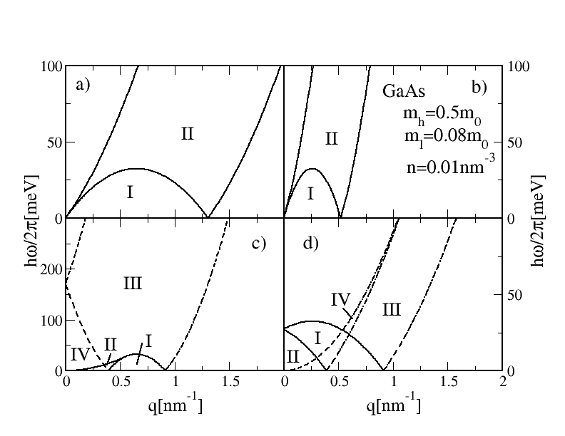
Figure 1: Regions of nonvanishing contributions to a): $I_{hh}(\vec{q},\omega)$, b): $I_{ll}(\vec{q},\omega)$, c): $I_{hl}^{+}(\vec{q},\omega)$ (solid lines) and $I_{hl}^{-}(\vec{q},\omega)$ (dashed lines), and d): $I_{lh}^{+}(\vec{q},\omega)$ (solid lines) and $I_{lh}^{-}(\vec{q},\omega)$ (dashed lines); cf. tables 1-3. We have chosen the mass parameters of GaAs, $m_{h}=0.5m_{0}$, $m_{l}=0.08m_{0}$, and a hole density of $n=0.01{\rm nm}^{-3}$.

IV The dielectric function

Let us now analyze the RPA dielectric function resulting from the above free polarizability. We first concentrate on the effect of the mass difference between heavy and light holes. To this end we eliminate effects of the dielectric background by putting $\varepsilon_{r}=1$, and we fix the total density $n=n_{h}+n_{l}$, $n_{h/l}=k_{h/l}^{3}/3\pi^{2}$, to $n=0.01{\rm nm}^{-3}$.

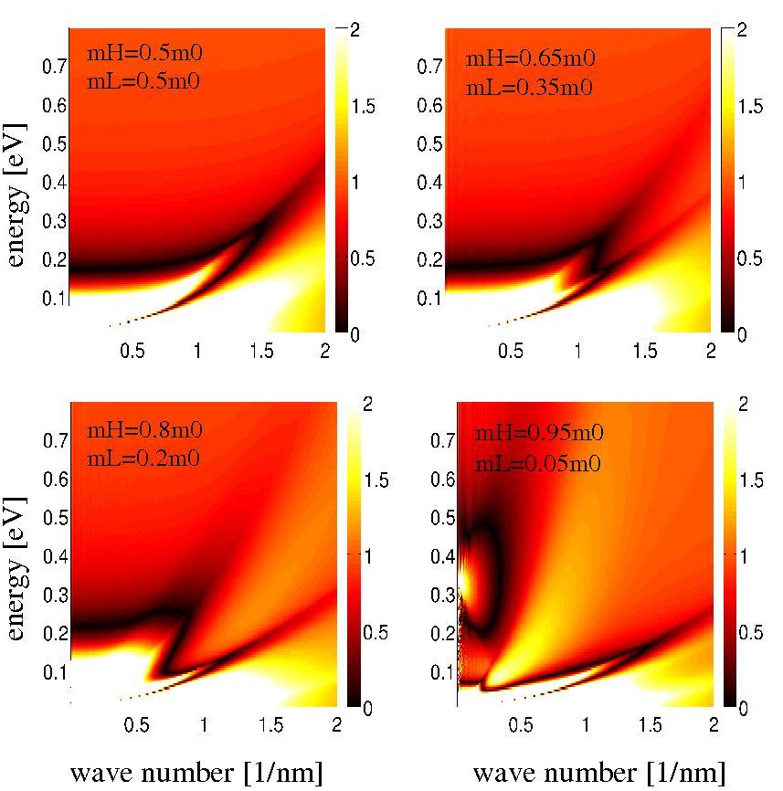
Figure 2: The modulus $|{\rm Re}(\varepsilon^{RPA}(\vec{q},\omega))|$ of the real part of the RPA dielectric function as a function of wave number $q$ and energy $\hbar\omega$ for a model system with $\varepsilon_{r}=1$. The ratio of heavy and light mass is varied at constant $m_{H}+m_{l}=m_{0}$, and the total hole density is $n=0.01{\rm nm}^{-3}$.

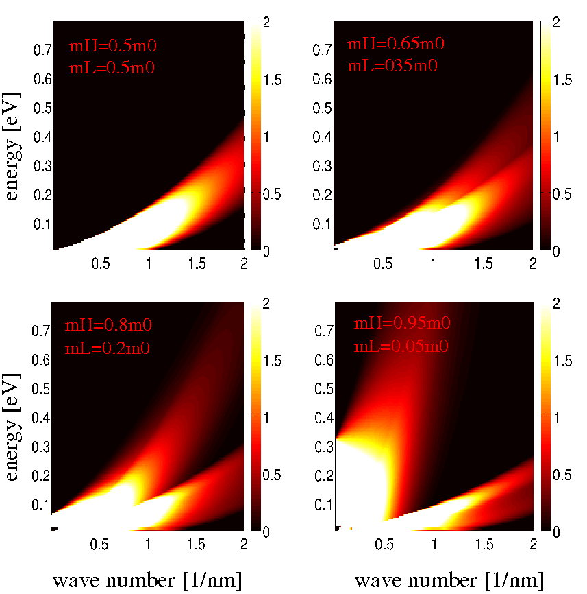
Figure 3: The imaginary part ${\rm Im}(\varepsilon^{RPA}(\vec{q},\omega))$ of the the RPA dielectric function as a function of wave number $q$ and energy $\hbar\omega$ for a model system with $\varepsilon_{r}=1$. The ratio of heavy and light mass is varied at constant $m_{H}+m_{l}=m_{0}$, and the total hole density is $n=0.01{\rm nm}^{-3}$.

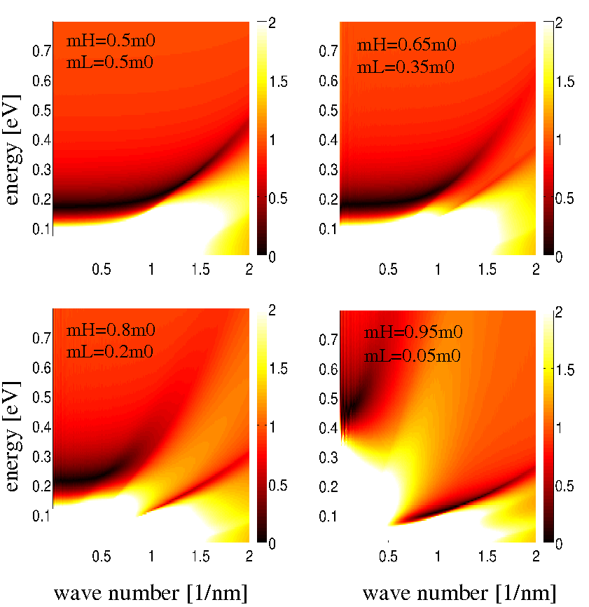
Figure 4: The modulus $|\varepsilon^{RPA}(\vec{q},\omega)|$ of the RPA dielectric function as a function of wave number $q$ and energy $\hbar\omega$ for a model system with $\varepsilon_{r}=1$. The ratio of heavy and light mass is varied at constant $m_{H}+m_{l}=m_{0}$, and the total hole density is $n=0.01{\rm nm}^{-3}$. The dark areas indicate zeros of the dielectric function corresponding to plasmon excitations.

Figs. 2, 3 show the realnotereal and imaginary part of the dielectric function as a function of wave number and frequency in a color-coded density plot, whereas in 4 the modulus of $\varepsilon^{RPA}(\vec{q},\omega)$ is shown. The top left panel in each figure illustrates the textbook caseGiuliani05 ; Mahan00 ; Bruus04 of equal masses $m_{H}=m_{l}=m_{0}/2$ with its well-known plasmon dispersion $\omega(q)$ determined by $\varepsilon^{RPA}(\vec{q},\omega(q))=0$. With increasing mass difference between heavy and light holes a more complex structure arises and the plasmon dispersion splits into two branches as seen in the bottom panels of Fig. 4: A branch with comparatively high energies at small wave numbers is accompanied by a branch at lower energies and large wave vectors. It is an interesting speculation whether one can interpret these two plasmon branches in analogy to phonons: On one branch both heavy and light holes possibly perform (speaking in classical terms) joint collective oscillations of charge density (analogous to acoustic phonons), while on the other branch they oscillate opposite to each other (similar to optical phonons). We leave this particular issue to future investigations.

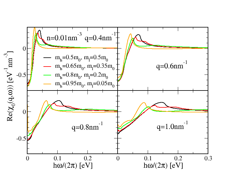
Figure 5: The real part of the free polarizability $\chi_{0}(\vec{q},\omega)$ as a function of frequency at different wave vectors for the same choice of heavy and light hole masses as in the previous figures.

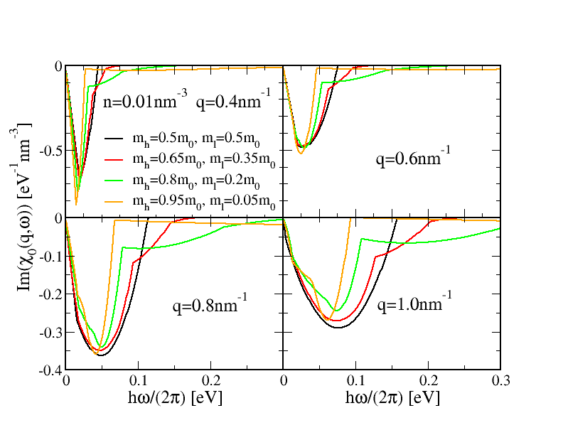
Figure 6: The imaginary part of the free polarizability $\chi_{0}(\vec{q},\omega)$ as a function of frequency at different wave vectors for the same choice of heavy and light hole masses as in the previous figures.

Finally, Figs. 5, 6 show the free polarizability as a function of frequency at different wave vectors for the same choice of heavy and light hole masses as in the previous figures.

Let us now discuss our results for the dielectric function with respect to concrete III-V semiconductors. In order to make contact to typical ferromagnetic semiconductor systemsJungwirth06 , and to compare with results of Ref.Kyrychenko11 we choose here a higher carrier density of $n=0.35{\rm nm}^{-3}$. We consider four typical III-V systems whose relevant parametersVurgaftman01 are given in table 4. Note that now also the background dielectric constant $\varepsilon_{r}$ plays a nontrivial role. In Figs. 7, 8, 9 we have plotted the realnotereal and imaginary part, and the modulus, respectively, of the dielectric function as a function of wave number and frequency. As seen from Fig. 9, the zeros of the dielectric function $\varepsilon^{RPA}(\vec{q},\omega)$ defining the plasmon excitations form a clearly more complex pattern than in the standard jellium liquid, and, as in the previous case, two dispersion branches can be identified. In particular, the plasmon excitation in GaAs at small wave vector occurs slightly below $0.3{\rm eV}$ which agrees very well with Fig. 4 of Ref.Kyrychenko11 where a more complex model for the band structure was used. However, differently from the findings there, we can identify two plasmon dispersion branches with small damping. Moreover, In Fig. 10 we show the free polarizability $\chi_{0}(\vec{q},\omega)$ as a function of frequency at different wave vectors for the same semiconductor systems. Again, the imaginary part for GaAs agrees nicely with data given in Fig. 2 of Ref.Kyrychenko11 . In this regime the imaginary part of the free polarizability is dominated by transitions between heavy-hole states, i.e. the main contributions is $I_{hh}(\vec{q},\omega)$, in accordance with Ref.Kyrychenko11 .

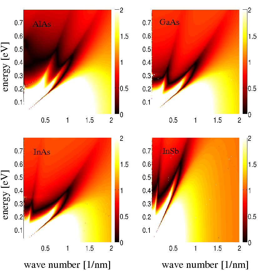
Figure 7: The modulus $|{\rm Re}(\varepsilon^{RPA}(\vec{q},\omega))|$ of the real part of the RPA dielectric function as a function of wave number $q$ and energy $\hbar\omega$ for various semiconductor systems at a total hole density of $n=0.35{\rm nm}^{-3}$.

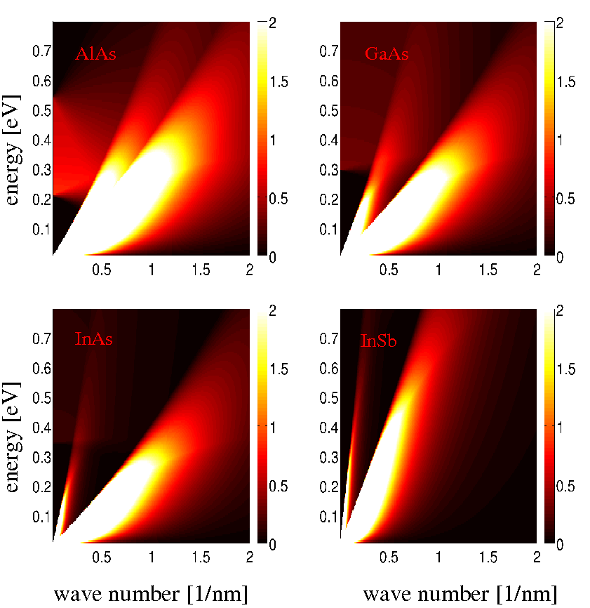
Figure 8: The imaginary part ${\rm Im}(\varepsilon^{RPA}(\vec{q},\omega))$ of the the RPA dielectric function as a function of wave number $q$ and energy $\hbar\omega$ for various semiconductor systems at a total hole density of $n=0.35{\rm nm}^{-3}$.

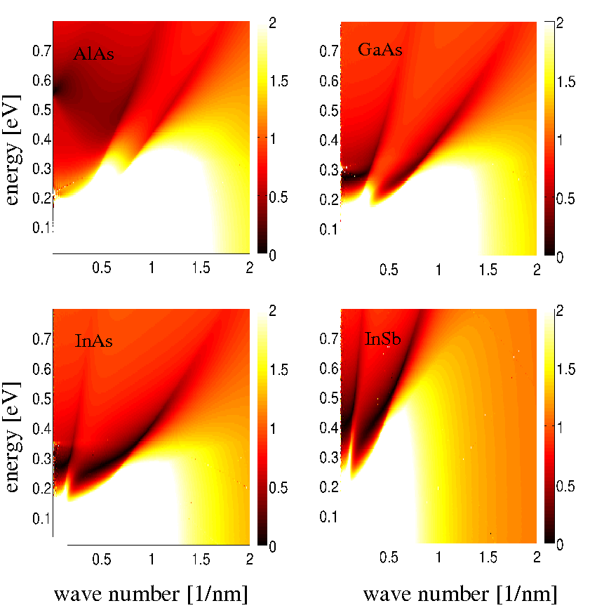
Figure 9: The modulus $|\varepsilon^{RPA}(\vec{q},\omega)|$ of the RPA dielectric function as a function of wave number $q$ and energy $\hbar\omega$ for various semiconductor systems at a total hole density of $n=0.35{\rm nm}^{-3}$. The dark areas indicate zeros of the dielectric function corresponding to plasmon excitations.

	$\frac{m_{h}}{m_{0}}$	$\frac{m_{l}}{m_{0}}$	$\varepsilon_{r}$
AlAs	0.47	0.18	10.0
GaAs	0.5	0.08	12.8
InAs	0.5	0.026	14.5
InSb	0.2	0.015	18.0

Table 4: Heavy and light hole masses long with background dielectric constants for various III-V semiconductorsVurgaftman01 .

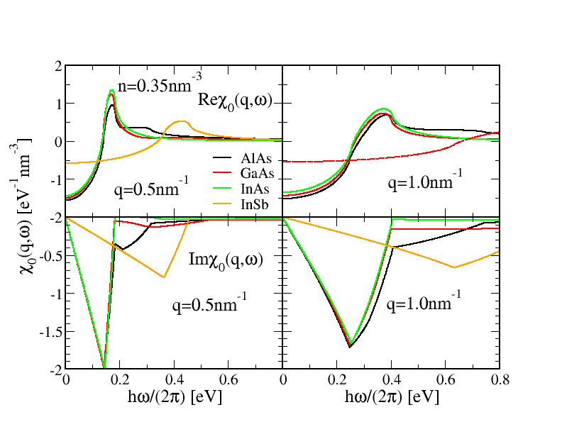
Figure 10: The real (top panels) and imaginary (bottom panels) part of the free polarizability $\chi_{0}(\vec{q},\omega)$ as a function of frequency at different wave vectors for the same semiconductor systems as before (cf. table 4).

IV.1 Static limit

In the static limit $\omega=0$, the rather complex contributions (22) to the free polarizability of the hole system simplify considerably to Schliemann10 ; notecorr1

$$\chi_{0}(\vec{q},0) = -\frac{m_{h}}{\pi^{2}\hbar^{2}}k_{h}\left(1+3\left(\frac{q}{2k_{h}}\right)^{2}\right)L\left(\frac{q}{2k_{h}}\right)$$ (39)

$$-\frac{m_{l}}{\pi^{2}\hbar^{2}}k_{l}\left(1+3\left(\frac{q}{2k_{l}}\right)^{2}\right)L\left(\frac{q}{2k_{l}}\right)$$

$$+\frac{3\left(\sqrt{m_{h}}+\sqrt{m_{l}}\right)^{2}}{4\pi^{2}\hbar^{2}}\frac{q^{2}}{k_{h}+k_{l}}L\left(\frac{q}{k_{h}+k_{l}}\right)$$

$$-\frac{3\left(m_{h}-m_{l}\right)}{4\pi^{2}\hbar^{2}}\left(k_{h}-k_{l}\right)\left(1-L\left(\frac{q}{k_{h}+k_{l}}\right)\right)$$

$$+\frac{3m_{h}}{2\pi^{2}\hbar^{2}}qH\left(\frac{q}{2k_{h}}\right)+\frac{3m_{l}}{2\pi^{2}\hbar^{2}}qH\left(\frac{q}{2k_{l}}\right)$$

$$-\frac{3\left(m_{h}+m_{l}\right)}{2\pi^{2}\hbar^{2}}qH\left(\frac{q}{k_{h}+k_{l}}\right)\,,$$

where $L(x)$ is the so-called Lindhard correction,

$$L(x)=\frac{1}{2}+\frac{1-x^{2}}{4x}\ln\left|\frac{1+x}{1-x}\right|\,,$$ (40)

and the function $H$ is defined as

$$H(x) = \frac{1}{2}\int_{0}^{1/x}dy\frac{1}{y}\ln\left|\frac{1+y}{1-y}\right|$$ (43)

$$= \left\{\begin{array}[]{ll}\frac{\pi^{2}}{4}-\sum_{n=0}^{\infty}\frac{x^{2n+1}}{(2n+1)^{2}}&|x|\leq 1\\ \sum_{n=0}^{\infty}\frac{\left(\frac{1}{x}\right)^{2n+1}}{(2n+1)^{2}}&|x|\geq 1\end{array}\right.\,.$$

Details of the derivation of the above result can be found in appendix A.1.1. Note that the static polarizability can entirely be expressed in terms of the arguments $k/2k_{h}$, $k/2k_{l}$, and $k/k_{h}+k_{l}$ with the latter one being the harmonic mean of the two former. In the case $m_{h}=m_{l}$ (i.e. $k_{h}=k_{l}=:k_{F}$) one obtains the usual result $\chi_{0}(\vec{q},0)=-D(\varepsilon_{F})L(q/2k_{F})$ for charge carriers without spin-orbit coupling where $D(\varepsilon)$ is the density of states Simion05 . For $m_{h}\neq m_{l}$, however, the static polarizability (39) has a clearly more complicated structure. Fig. 11 displays the static free polarizability and dielectric function for the systems discussed above. In particular, the data in the left panel at fixed $m_{h}+m_{l}=m_{0}$ shows that the static polarizability develops richer features with increasing difference in heavy and light hole mass.

Moreover, in the long-wave approximation $\chi_{0}(\vec{q},0)\approx\chi_{0}(0,0)$ one recovers the usual Thomas-Fermi (TF) screening,

$$\varepsilon^{RPA}(\vec{q},0)\approx 1-q^{2}_{TF}/q^{2}$$ (44)

with a Thomas-Fermi wave number $q^{2}_{TF}=(e^{2}/\varepsilon_{r}\varepsilon_{0})3n/(2\varepsilon_{f})$.

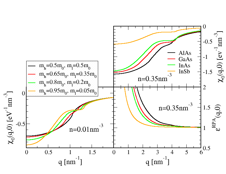
Figure 11: Left panel: The static free polarizability $\chi_{0}(\vec{q},0)$ for the same choice of parameters as in Figs. 2-6. Right panels: $\chi_{0}(\vec{q},0)$ and $\varepsilon^{RPA}(\vec{q},0)$ the same III-V semiconductor systems as in Figs. 7-10 (cf. table 4).

As discussed in Ref. Schliemann10 , the full screened potential of a pointlike probe charge $Q$,

$$\Phi(\vec{r})=\frac{1}{(2\pi)^{3}}\int d^{3}q\frac{\frac{Q}{\varepsilon_{r}\varepsilon_{0}q^{2}}}{\varepsilon^{RPA}(\vec{q})}e^{i\vec{q}\vec{r}}$$ (45)

can conveniently be approximated using Lighthill’s theorem Lighthill58 as

$$\Phi(r)\approx\frac{m_{h}}{m_{0}}\phi_{\infty}(2k_{h},r)+\frac{m_{l}}{m_{0}}\phi_{\infty}(2k_{l},r)$$ (46)

where

$$\phi_{\infty}(q,r)=\frac{Q}{4\pi\varepsilon_{0}a_{0}}\frac{2}{\pi}\frac{1}{\left(\varepsilon_{r}\varepsilon^{RPA}(q)\right)^{2}}\frac{\cos(qr)}{(qr)^{3}}$$ (47)

and $a_{0}=4\pi\varepsilon_{0}\hbar^{2}/(m_{0}e^{2})$ being the usual Bohr radius. As a result, a beating of Friedel oscillations between the two wave numbers $2k_{h/l}$ (but not $k=(k_{h}+k_{l})/2$) takes placeSchliemann10 . This beating is a peculiarity of the holes residing in the p-type valence band and should be observable via similar scanning tunneling microscopy techniques as used in metals Crommie93 and $n$-doped semiconductors Kanisawa01 . Moreover, as theoretical studies have revealed, such oscillations can have a profound impact on the magnetic properties of ferromagnetic semiconductors by giving way to the possibility of noncollinear magnetic orderingSchliemann02 ; Fiete05 .

IV.2 Limit of large frequencies

In the regime of large frequencies and small wave vectors. one can expand the denominators in Eq. (18) assuming $\hbar\omega>>\varepsilon_{h/l}(\vec{q})$ and $\hbar\omega>>(\hbar k_{h/l}/m_{h/l})\hbar q$. The result within the two leading orders readsSchliemann10 ; notecorr2

$$\varepsilon^{RPA}(\vec{q},\omega)=1-\frac{1}{\omega^{2}}\frac{e^{2}}{\varepsilon_{r}\varepsilon_{0}}\frac{1}{6\pi^{2}}\left(\frac{1}{m_{h}}+\frac{1}{m_{l}}\right)\left(k_{h}^{3}+k_{l}^{3}\right)$$

$$\qquad-\frac{1}{\omega^{4}}\frac{e^{2}\hbar^{2}}{\varepsilon_{r}\varepsilon_{0}\pi^{2}}\frac{1}{2}\left(\frac{1}{m_{h}^{3}}+\frac{1}{m_{l}^{3}}\right)\Biggl{[}\frac{1}{5}q^{2}\left(k_{h}^{5}+k_{l}^{5}\right)$$

$$\qquad\qquad+\frac{1}{12}q^{4}\left(k_{h}^{3}+k_{l}^{3}\right)\Biggr{]}$$

$$\qquad-\frac{1}{\omega^{4}}\frac{e^{2}\hbar^{2}}{\varepsilon_{r}\varepsilon_{0}\pi^{2}}\Biggl{[}-\frac{1}{56}\left(\frac{1}{m_{h}}-\frac{1}{m_{l}}\right)^{3}\left(k_{h}^{7}-k_{l}^{7}\right)$$

$$\qquad\qquad+\frac{21}{200}q^{2}\left(\frac{1}{m_{h}^{3}}-\frac{1}{m_{l}^{3}}\right)\left(k_{h}^{5}-k_{l}^{5}\right)$$

$$\qquad\qquad-\frac{3}{40}q^{2}\left(\frac{1}{m_{h}}-\frac{1}{m_{l}}\right)\left(\frac{k_{h}^{5}}{m_{l}^{2}}-\frac{k_{l}^{5}}{m_{h}^{2}}\right)\Biggr{]}$$ (48)

For $m_{h}=m_{l}$ the first three lines of the above expression reproduce again the standard textbook result Mahan00 while all other terms vanish in this limit. On the other hand, if $m_{h}\neq m_{l}$, contributions in order $1/\omega^{4}$ occur that are independent of the wave vector $\vec{q}$. Such terms are absent in the case of the standard electron gas where the contributions of order $1/\omega^{2n}$ are at least of order $q^{2n-2}$ in the wave vector Mahan00 . The technical reason why such contributions are present for the hole gas is that the expression $\varepsilon_{\lambda_{2}}(\vec{k}+\vec{q})-\varepsilon_{\lambda_{1}}(\vec{k})$ in Eq.(18) contains for $|\lambda_{1}|\neq|\lambda_{2}|$ an additive term which is independent of $k$ (and vanishes for $m_{h}=m_{l}$). As a consequence, although the result (48) is the valid high frequency expansion of the dielectric function, it is not possible to obtain from it a reliable expression for the plasmon dispersion $\omega(q)$ defined by $\varepsilon^{RPA}(\vec{q},\omega(q))=0$. This statement holds even for the long-wavelength plasma frequency $\omega(q=0)$ and is due to the fact that in any order in $(1/\omega^{2})$ the prefactor in the expansion contains contributions being of low order (including zeroth order) in $q$. As an example, relying on the expansion (48) being of up to quartic order in $1/\omega$, the condition $\varepsilon^{RPA}(\vec{q},\omega(q))=0$ translates toSchliemann10 ; notecorr2

$$\omega^{2}(q)=\left(\omega_{p}^{(0)}\right)^{2}\Biggl{[}\frac{1}{2}+\frac{1}{2}\Bigl{[}1+4\Bigl{(}u\left(n^{1/3}a_{0}\right)$$

$$\qquad\qquad+\left(v+w\right)\frac{(qa_{0})^{2}}{n^{1/3}a_{0}}\Bigr{)}\Bigr{]}^{1/2}\Biggr{]}+{\cal O}\left(q^{4}\right)\,.$$ (49)

Here we have defined

$$\left(\omega_{p}^{(0)}\right)^{2}=\frac{e^{2}}{\varepsilon_{r}\varepsilon_{0}}\frac{n}{2}\left(\frac{1}{m_{h}}+\frac{1}{m_{l}}\right)\,,$$ (50)

and the density-independent coefficients $u$, $v$, and $w$ are given by

$$u=\frac{-Q\left(m_{h},m_{l}\right)}{\left(3\pi^{2}\right)^{1/3}\left(m_{h}^{3/2}+m_{l}^{3/2}\right)^{2/3}}$$

$$\quad\times\frac{3}{14}\left(\frac{1}{m_{h}}-\frac{1}{m_{l}}\right)^{3}\left(m_{h}^{7/2}-m_{l}^{7/2}\right)\,,$$ (51)

$$v=\frac{2Q\left(m_{h},m_{l}\right)}{5\pi^{2}}\left(\frac{1}{m_{h}^{3}}+\frac{1}{m_{l}^{3}}\right)\left(m_{h}^{5/2}+m_{l}^{5/2}\right)\,,$$ (52)

$$w=\frac{3Q\left(m_{h},m_{l}\right)}{10\pi^{2}}\Biggl{[}\frac{7}{5}\left(\frac{1}{m_{h}^{3}}-\frac{1}{m_{l}^{3}}\right)\left(m_{h}^{5/2}-m_{l}^{5/2}\right)$$

$$\qquad\qquad-\left(\frac{1}{m_{h}}-\frac{1}{m_{l}}\right)\left(\frac{m_{h}^{5/2}}{m_{l}^{2}}-\frac{m_{l}^{5/2}}{m_{h}^{2}}\right)\Biggr{]}$$ (53)

with the common prefactor

$$Q\left(m_{h},m_{l}\right)=\frac{\frac{\varepsilon_{r}}{4\pi}m_{0}}{\left(\frac{1}{m_{h}}+\frac{1}{m_{l}}\right)^{2}}\frac{(3\pi^{2})^{5/3}}{\left(m_{h}^{3/2}+m_{l}^{3/2}\right)^{5/3}}\,.$$ (54)

Clearly, the coefficients $u$ and $w$ vanish for $m_{h}=m_{l}$ while from $v$ one recovers usual textbook result for an electron gas without spin-orbit coupling Mahan00 . However, if $m_{h}$ and $m_{l}$ differ substantially, the neglected contributions occurring in higher order in the inverse frequency but being independent of or of low order in the wave vector can substantially modify the plasmon excitations. This can even affect the plasma frequency $\omega(q=0)$ at zero wave vector: E.g. for the parameters of GaAs (cf. table 4) and a total hole density of $n=0.35{\rm nm}^{-3}$ one obtains from Eq. (49) $\hbar\omega(q=0)\approx 0.8{\rm eV}$, in contrast to the value of slightly less than $0.3{\rm eV}$ found from a full evaluation of the dielectric function (cf. Fig. 9 top right panel) which is also in accordance with Ref.Kyrychenko11 . In summary, although the expansion 48 is the correct description of the dielectric function in the limit of large frequencies, it does not lead to reliable expressions for the plasmon dispersion. This is due to peculiarities of the expansion occurring for $m_{h}\neq m_{l}$. On the other hand, as seen from e.g. Fig. 9, the interplay between the hole mass difference and the background dielectric constant leads to plasmon excitations patterns which differ dramatically from the textbook case of the jellium model. This alternations, however, are not accurately described by expressions of the type (49), in contrast to an earlier approach where results for the full wave vector and frequency dependence of the dielectric function were not available yetSchliemann10 .

V Conclusions and outlook

We have investigated the RPA dielectric function of the homogeneous semiconductor hole liquid in $p$-doped bulk III-V zinc-blende semiconductors. The single-particle physics of the hole system is modeled by Luttinger’s four-band Hamiltonian in its spherical approximation. Regarding the Coulomb-interacting hole liquid, the full dependence of the zero-temperature dielectric function on wave vector and frequency has been explored. The imaginary part of the dielectric function is analytically obtained in terms of complicated but fully elementary expressions, while in the result for the real part nonelementary one-dimensional integrations remain to be performed. The correctness of these two independent calculations is checked via Kramers-Kronig relations.

The mass difference between heavy and light holes, along with variations in the background dielectric constant, leads to dramatic alternations in the plasmon excitation pattern, and generically, two plasmon branches can be identified. These findings are the result of the evaluation of the full dielectric function and are not accessible via a high-frequency expansion. In the static limit a beating of Friedel oscillations between the Fermi wave numbers of heavy and light holes occurs.

Regarding future developments, possible extensions of the present work could include the implementation of more general single-particle Hamiltonians modeling the band structure. For instance, one could drop the spherical approximation to the Luttinger Hamiltonian and consider parameters $\gamma_{2}\neq\gamma_{3}$. However, such a reduction of the full rotational invariance to tetrahedral symmetry might prohibit analytical progress as achieved here. However, we do not expect drastic effects from such a generalization, in particular not since for the generic material GaAs $\gamma_{2}$, $\gamma_{3}$ are very close to each otherVurgaftman01 . Moreover, our results obtained here for the spherically symmetric $4\times 4$ valence band Hamiltonian agree, where overlapping, very reasonably with findings in Ref. Kyrychenko11 where a more complicated $8\times 8$ band structure model was evaluated numerically.

Having in mind ferromagnetic semiconductors such as Mn-doped GaAs, another obvious extension would be a coupling to the hole spins by a homogeneous Zeeman-type field mimicking the magnetization of the Mn ions. A technical difficulty here lies in the fact that the resulting single-particle Hamiltonian cannot be diagonalized any more in a convenient analytical fashion. However, analytical progress might still be possible if the Zeeman coupling is treated as a perturbation. This strategy leads of course to also consider the spin susceptibility, i.e. spin-spin response function. For a standard jellium systems of spin-$1/2$ fermions without spin-orbit coupling, this quantity is, up to constant prefactors, identical to the free electrical polarizationGiuliani05 . For the $4\times 4$ hole system studied here, however, this simple relation is rendered invalid by the larger spin length and, more importantly, the presence of manifest spin-orbit coupling. Thus, a study of the spin susceptibility in a similarly analytical fashion as done here for the electric polarizability and the dielectric function appears also to be useful.

Finally, from the point of view of general many-particle physics, the inclusion of so-called local many-body field factors would be an important step towards correlations beyond RPAGiuliani05 . The practical treatment of such local field factors in the presence of strong spin-orbit coupling, however, is still in its infancy.

Appendix A Calculation of the free polarizability

A.1 The real part

With the help of the Dirac identity

$$\frac{1}{x+i0}={\cal P}\frac{1}{x}-i\pi\delta(x)$$ (55)

the contributions to the real part of the free polarizability of the hole gas read

$$R_{hh}(\vec{q},\omega) = \frac{-1}{(2\pi\hbar)^{2}}\frac{m_{h}}{q^{2}}{\cal P}\int_{0}^{k_{h}}dkk^{2}\int_{-1}^{1}dx\left(1+3\frac{k^{2}+2kqx+q^{2}x^{2}}{k^{2}+2kqx+q^{2}}\right)$$ (56)

$$\qquad\qquad\qquad\times\left[\frac{1}{1+(2k/q)x-2m_{h}\omega/(\hbar q^{2})}+\left(\omega\mapsto-\omega\right)\right]\,,$$

$$R_{hl}(\vec{q},\omega) = \frac{-1}{(2\pi\hbar)^{2}}\frac{m_{l}}{q^{2}}{\cal P}\int_{0}^{k_{h}}dkk^{2}\int_{-1}^{1}dx\left(3-3\frac{k^{2}+2kqx+q^{2}x^{2}}{k^{2}+2kqx+q^{2}}\right)$$ (57)

$$\qquad\qquad\qquad\times\left[\frac{1}{1+(2k/q)x+(1-m_{l}/m_{h})k^{2}/q^{2}-2m_{l}\omega/(\hbar q^{2})}+\left(\omega\mapsto-\omega\right)\right]\,.$$

The integration over the polar variable $x$ can be performed by applying the identity

$$\frac{k^{2}+2kqx+q^{2}x^{2}}{k^{2}+2kqx+q^{2}}\frac{1}{1+(2k/q)x+\alpha} = \left(\frac{q}{2k}\right)^{2}-\frac{q/(8k)}{1-(q/k)^{2}\alpha}\left(1-\frac{q^{2}}{k^{2}}\right)\frac{1}{x+q/(2k)+k/(2q)}$$ (58)

$$+\frac{q/(2k)}{1-(q/k)^{2}\alpha}\left(1-\frac{q^{2}}{2k^{2}}(1+\alpha)\right)^{2}\frac{1}{x+q(1+\alpha)/(2k)}$$

for $\alpha=-2m_{h}\omega/(\hbar q^{2})$ and $\alpha=(1-m_{l}/m_{h})k^{2}/q^{2}-2m_{l}\omega/(\hbar q^{2})$. Adding both contributions, and introducing a dimensionless radial integration variable $y=2k/q$, the result can be formulated as

$$R_{hh}(\vec{q},\omega)+R_{hl}(\vec{q},\omega) = \frac{-1}{(2\pi\hbar)^{2}}\frac{q}{4}{\cal P}\int_{0}^{2k_{h}/q}dyy^{2}\Biggl{[}\frac{m_{h}}{2}\frac{1}{y}\ln\left|\frac{1-2m_{h}\omega/(\hbar q^{2})+y}{1-2m_{h}\omega/(\hbar q^{2})-y}\right|+\frac{3}{y^{2}}(m_{h}-m_{l})$$ (59)

$$+\frac{3m_{l}}{2}\frac{1}{y}\ln\left|\frac{1-2m_{l}\omega/(\hbar q^{2})+y+(1-m_{l}/m_{h})y^{2}/4}{1-2m_{l}\omega/(\hbar q^{2})-y+(1-m_{l}/m_{h})y^{2}/4}\right|$$

$$+\frac{3m_{h}}{2}\frac{y}{y^{2}+8m_{h}\omega/(\hbar q^{2})}\left(1-\frac{2}{y^{2}}\left(1-\frac{2m_{h}\omega}{\hbar q^{2}}\right)\right)^{2}\ln\left|\frac{1-2m_{h}\omega/(\hbar q^{2})+y}{1-2m_{h}\omega/(\hbar q^{2})-y}\right|$$

$$-\frac{3m_{h}}{2}\frac{y}{y^{2}+8m_{h}\omega/(\hbar q^{2})}\left(\frac{1}{2}\left(1+\frac{m_{l}}{m_{h}}\right)-\frac{2}{y^{2}}\left(1-\frac{2m_{l}\omega}{\hbar q^{2}}\right)\right)^{2}$$

$$\qquad\qquad\times\ln\left|\frac{1-2m_{l}\omega/(\hbar q^{2})+y+(1-m_{l}/m_{h})y^{2}/4}{1-2m_{l}\omega/(\hbar q^{2})-y+(1-m_{l}/m_{h})y^{2}/4}\right|+\left(\omega\mapsto-\omega\right)\Biggr{]}$$

Now, by rearranging the terms in the integrand and performing elementary integrations, one obtains the result (22). We note that also the integral in the third line of Eq. (22) is elementary but lengthy,

$$\int_{0}^{x}dy\,y\ln\left|\frac{ay^{2}+by+c}{ay^{2}-by+c}\right| = \frac{1}{2}\left(x^{2}-\frac{b^{2}}{2a^{2}}+\frac{c}{a}\right)\ln\left|\frac{ay^{2}+by+c}{ay^{2}-by+c}\right|+\frac{b}{a}x$$ (61)

$$- \left\{\begin{array}[]{ll}\frac{b}{a}\sqrt{\frac{b^{2}}{4a^{2}}-\frac{c}{a}}\left(\tanh^{-1}\left(\frac{x+b/(2a)}{\sqrt{b^{2}/(4a^{2})-c/a}}\right)+\tanh^{-1}\left(\frac{x-b/(2a)}{\sqrt{b^{2}/(4a^{2})-c/a}}\right)\right)&\frac{b^{2}}{4a^{2}}-\frac{c}{a}\geq 0\\ \frac{b}{a}\sqrt{\frac{c}{a}-\frac{b^{2}}{4a^{2}}}\left(\tan^{-1}\left(\frac{x+b/(2a)}{\sqrt{c/a-b^{2}/(4a^{2})}}\right)+\tan^{-1}\left(\frac{x-b/(2a)}{\sqrt{c/a-b^{2}/(4a^{2})}}\right)\right)&\frac{b^{2}}{4a^{2}}-\frac{c}{a}\leq 0\end{array}\right.\,,$$

whereas all other integrals in Eq. (22) cannot be expressed via elementary functions.

A.1.1 Static limit

In the static limit $\omega\to 0$ one obtains from Eq. (22) (or, alternatively, Eq. (59))

$$R_{hh}(\vec{q},0)+R_{hl}(\vec{q},0) = \frac{-m_{h}}{(2\pi\hbar)^{2}}\left(2k_{h}+\frac{q/2}{\varepsilon_{h}(q)}\left(\varepsilon_{f}-\varepsilon_{h}(q)\right)\ln\left|\frac{\varepsilon_{h}(q)+\hbar^{2}qk_{h}/m_{h}}{\varepsilon_{h}(q)-\hbar^{2}qk_{h}/m_{h}}\right|\right)-\frac{3}{(2\pi\hbar)^{2}}\left(m_{h}-m_{l}\right)k_{h}$$ (62)

$$+ \frac{3}{(2\pi\hbar)^{2}}\frac{m_{h}q}{16}\left(1-\frac{m_{h}}{m_{l}}\right)^{2}\sum_{\mu=\pm}y_{\mu}^{2}\int_{0}^{2k_{h}/(qy_{\mu})}dyy\ln\left|\frac{1+y}{1-y}\right|$$

$$+ \frac{3}{(2\pi\hbar)^{2}}m_{h}q\int_{0}^{2k_{h}/q}dy\frac{1}{y}\ln\left|\frac{1+y}{1-y}\right|-\frac{3/2}{(2\pi\hbar)^{2}}\left(m_{h}+m_{l}\right)\sum_{\mu=\pm}\int_{0}^{2k_{h}/(qy_{\mu})}dy\frac{1}{y}\ln\left|\frac{1+y}{1-y}\right|$$

$$- \frac{3}{(2\pi\hbar)^{2}}m_{h}q\int_{0}^{2k_{h}/q}dy\frac{1}{y^{3}}\left(\ln\left|\frac{1+y}{1-y}\right|-\ln\left|\frac{1+y/y_{+}}{1-y/y_{+}}\right|-\ln\left|\frac{1+y/y_{-}}{1-y/y_{-}}\right|\right)\,,$$

where we have split a part of the logarithmic terms in the integrand by introducing $y_{\pm}:=2/(1\pm\sqrt{m_{l}/m_{h}})$. In order to simplify the above expression we first note that the first term of the r.h.s can be written as $-m_{h}L(q/(2k_{h}))/(\pi\hbar)^{2}$ using the Lindhard correction (40). Regarding the terms in the second and third line involving a summation over $\mu=\pm$, the interchange $h\leftrightarrow l$ leads to $y_{\pm}\leftrightarrow\bar{y}_{\pm}:=2/(1\pm\sqrt{m_{h}/m_{l}})$ fulfilling $2k_{l}/(q\bar{y}_{\pm})=\pm 2k_{h}/(qy_{\pm})$ and $m_{h}\bar{y}_{\pm}^{2}=m_{l}y_{\pm}^{2}$. From these observations it is easy to see that the terms with $\mu=-$ cancel against corresponding expressions in $R_{ll}(\vec{q},0)+R_{lh}(\vec{q},0)$, and only the terms with $\mu=+$ (being invariant under $h\leftrightarrow l$) contribute to $\chi_{0}(\vec{q},0)$. The first of these contributions (second line in Eq. (62)) can be expressed again via the Lindhard correction, while the integrals in the third line involve the function $H(x)$ defined in Eq. (43). Finally, the last line of Eq. (62) can be evaluated as

$$m_{h}\int_{0}^{2k_{h}/q}dy\frac{1}{y^{3}}\left(\ln\left|\frac{1+y}{1-y}\right|-\ln\left|\frac{1+y/y_{+}}{1-y/y_{+}}\right|-\ln\left|\frac{1+y/y_{-}}{1-y/y_{-}}\right|\right)$$ (63)

$$= 2m_{h}\frac{q}{2k_{h}}L\left(\frac{q}{2k_{h}}\right)-\frac{\left(\sqrt{m_{h}}+\sqrt{m_{l}}\right)^{2}}{2}\frac{q}{k_{h}+k_{l}}L\left(\frac{q}{k_{h}+k_{l}}\right)-\frac{\left(\sqrt{m_{h}}-\sqrt{m_{l}}\right)^{2}}{2}\frac{q}{k_{h}-k_{l}}L\left(\frac{q}{k_{h}-k_{l}}\right)\,,$$

where the last term on the r.h.s. is odd under $h\leftrightarrow l$ and cancels agianst an analogous contribution in $R_{ll}(\vec{q},0)+R_{lh}(\vec{q},0)$. Now summing all expressions one ends up with the result (39) for the free polarizability $\chi_{0}(\vec{q},0)$.

A.2 The imaginary part

A.2.1 $I_{hh}(\vec{q},\omega)$ and $I_{ll}(\vec{q},\omega)$

Using the Dirac identity (55) and performing the angular integrations, $I_{hh}(\vec{q},\omega)$ can be expressed as

$$I_{hh}(\vec{q},\omega) = \frac{-1}{4\pi q}\frac{m_{h}}{\hbar^{2}}\int_{0}^{k_{h}}dk\Biggl{[}\left(2k+\frac{3}{2k}\frac{(q^{2}/2+m_{h}\omega/\hbar)^{2}-q^{2}k^{2}}{k^{2}-2m_{h}\omega/\hbar}\right)\Theta\left(k-\left|\frac{q}{2}+\frac{m_{h}\omega}{\hbar q}\right|\right)$$ (64)

$$\qquad\qquad\qquad-\left(2k+\frac{3}{2k}\frac{(q^{2}/2-m_{h}\omega/\hbar)^{2}-q^{2}k^{2}}{k^{2}+2m_{h}\omega/\hbar}\right)\Theta\left(k-\left|\frac{q}{2}-\frac{m_{h}\omega}{\hbar q}\right|\right)\Biggr{]}\,,$$

where $\Theta(x)$ denotes the Heaviside step function. Obviuosly, the step functions occurring in the above expression define the lower integration bound, and the pertaining discussion parallels the arguments appropriate for the standard textbook case of a spinless Jellium model Giuliani05 ; Mahan00 ; Bruus04 . However, for the sake of completeness, and in order to point out important differences regarding the remaining quantities $I_{hl}(\vec{q},\omega)$ and $I_{lh}(\vec{q},\omega)$ to be analyzed below, let us briefly go into some details. Since $I_{hh}(\vec{q},-\omega)=-I_{hh}(\vec{q},\omega)$ it is sufficient to concentrate on $\omega\geq 0$. Then, if the first step function in (64) leads to a non-zero contribution (i.e. has a positive argument for some $k\in[0,k_{h}]$), this holds also for the second step function. Thus, a necessary and sufficient condition for both step function to contribute is $k_{h}-|q/2+m_{h}\omega/(\hbar q)|\geq 0$, which is equivalent to

$$\hbar q\frac{\hbar k_{h}}{m_{h}}-\varepsilon_{h}(q)\geq\hbar\omega$$ (65)

and can for non-negative frequencies only be fulfilled for $q\leq 2k_{h}$. The last two inequalities define region I in table 1, and the corresponding expression (23) is obtained by elementary integration.

Let us now turn to the case where only the second step function contributes, i.e. $k_{h}-|q/2-m_{h}\omega/(\hbar q)|\geq 0$ while inequality (65) is violated. Assuming $\hbar\omega\geq\varepsilon_{h}(q)$ we arrive at the condition

$$\hbar q\frac{\hbar k_{h}}{m_{h}}+\varepsilon_{h}(q)\geq\hbar\omega\geq\hbar q\frac{\hbar k_{h}}{m_{h}}-\varepsilon_{h}(q)\,,$$ (66)

while the opposite assumption, $\hbar\omega\leq\varepsilon_{h}(q)$, leads to

$$\hbar\omega\geq-\hbar q\frac{\hbar k_{h}}{m_{h}}+\varepsilon_{h}(q)\,.$$ (67)

The latter inequality is only a nontrivial condition if its r.h.s. is non-negative which is equivalent to $q\geq 2k_{h}$. In summary, the second step function in expression (64) contributes while the first one yields zero if, and only if, (i) $q\leq 2k_{h}$ and inequality (66) is fulfilled, or (ii) $q\geq 2k_{h}$ and

$$\hbar q\frac{\hbar k_{h}}{m_{h}}+\varepsilon_{h}(q)\geq\hbar\omega\geq-\hbar q\frac{\hbar k_{h}}{m_{h}}+\varepsilon_{h}(q)\,.$$ (68)

The above conditions define region II in table 1, and and the corresponding expression (24) follows again from elementary integration.

The remaining quantity $I_{ll}(\vec{q},\omega)$ is obtained from the above results via the replacement $h\mapsto l$.

A.2.2 $I_{hl}(\vec{q},\omega)$

After performing the angular integrations, $I_{hl}(\vec{q},\omega)$ can be formulated in the form (25) with

$$I_{hl}^{\pm}(\vec{q},\omega) = \frac{3}{8\pi q}\frac{m_{h}}{\hbar^{2}}\int_{0}^{k_{h}}dk\Biggl{[}\frac{1/k}{k^{2}\mp 2m_{h}\omega/\hbar}\Biggl{(}-\left(\frac{q^{2}}{2}\pm\frac{m_{l}\omega}{\hbar}\right)^{2}+k^{2}\left(q^{2}-\left(1-\frac{m_{l}}{m_{h}}\right)\left(\frac{q^{2}}{2}\pm\frac{m_{l}\omega}{\hbar}\right)\right)$$ (69)

$$\qquad\qquad\qquad\qquad-\frac{k^{4}}{4}\left(1-\frac{m_{l}}{m_{h}}\right)^{2}\Biggr{)}\Theta\left(k-\left|\frac{q}{2}+\left(1-\frac{m_{l}}{m_{h}}\right)\frac{k^{2}}{2q}\pm\frac{m_{l}\omega}{\hbar q}\right|\right)\Biggr{]}\,.$$

We now have to discuss under which circumstances the step functions in the above expression lead to nonzero contributions. This is more complicated than in the previous case since the arguments of the step functions depend quadratically (and not only linearly) on the integration variable $k$. The condition

$$\Theta\left(k-\left|\frac{q}{2}+\left(1-\frac{m_{l}}{m_{h}}\right)\frac{k^{2}}{2q}\pm\frac{m_{l}\omega}{\hbar q}\right|\right)=1$$ (70)

is equivalent to

$$(k+a)^{2}\geq b_{\pm}\quad\wedge\quad(k-a)^{2}\leq b_{\pm}$$ (71)

where we have defined

$$a = \frac{q}{1-m_{l}/m_{h}}\,,$$ (72)

$$b_{\pm} = a^{2}-\frac{2q}{1-m_{l}/m_{h}}\left(\frac{q}{2}\pm\frac{m_{l}\omega}{\hbar q}\right)$$ (73)

$$= \frac{(m_{l}/m_{h})q^{2}}{(1-m_{l}/m_{h})^{2}}\mp\frac{2m_{l}\omega/\hbar}{1-m_{l}/m_{h}}\,.$$

Here and in what follows the upper (lower) sign refers always to $I_{hl}^{+}(\vec{q},\omega)$ ($I_{hl}^{-}(\vec{q},\omega)$). Note that the step function in $I_{hl}^{+}(\vec{q},\omega)$ can, for non-negative frequencies, only be nonzero if this is also the case for $I_{hl}^{-}(\vec{q},\omega)$.

Since $m_{l}<m_{h}$ we clearly have $a\geq 0$, and the second inequality in (71) requires $b_{\pm}\geq 0$ which leads for the upper sign to the condition

$$\hbar\omega\leq\frac{1}{1-m_{l}/m_{h}}\varepsilon_{h}(q)\,.$$ (74)

Moreover, an elementary discussion of the inequalities (71) yields the following lower and upper boundaries for the integral (69) after resolving the step function,

$$\underline{l}_{\pm} = \min\left\{|a-\sqrt{b_{\pm}}|,k_{h}\right\}\,,$$ (75)

$$\overline{l}_{\pm} = \min\left\{a+\sqrt{b_{\pm}},k_{h}\right\}\,,$$ (76)

with $0\leq\underline{l}_{\pm}\leq\overline{l}_{\pm}\leq k_{h}$. Nonzero contributions occur only for $\underline{l}_{\pm}<k_{h}$. For the upper sign, the condition $\underline{l}_{\pm}\geq k_{h}$ implies

$$\hbar q\frac{\hbar k_{h}}{m_{l}}-\varepsilon_{l}(q)-\left(\frac{m_{h}}{m_{l}}-1\right)\varepsilon_{f}\leq\hbar\omega$$ (77)

which is, for non-negative $\omega$, a nontrivial statement on if

$$\left(1-\sqrt{m_{l}/m_{h}}\right)k_{h}\leq q\leq\left(1+\sqrt{m_{l}/m_{h}}\right)k_{h}\,.$$ (78)

Conversely, inequality (77) implies $\underline{l}_{\pm}\geq k_{h}$ only for $a\leq k_{h}$, while in the case $a\geq k_{h}$, i.e.

$$q\leq\left(1-m_{l}/m_{h}\right)k_{h}\,,$$ (79)

it follows $k_{h}\leq a+\sqrt{b_{+}}$, and the inequality (74) limits the region of nonzero $I_{hl}^{+}(\vec{q},\omega)$. The inequalities (79), (77), and (74) define region II in table 2 with the integration bounds being $\underline{l}_{+}=|a-\sqrt{b_{+}}|=:\underline{k}_{h}^{+}$ and $\overline{l}_{+}=a+\sqrt{b_{+}}=:\overline{k}_{h}^{+}$ as defined in Eqs. (29),(30). On the other hand, inequality (78) along with the negation of (77),

$$\hbar q\frac{\hbar k_{h}}{m_{l}}-\varepsilon_{l}(q)-\left(\frac{m_{h}}{m_{l}}-1\right)\varepsilon_{f}\geq\hbar\omega\,,$$ (80)

define region I in table 2. Here again $\underline{l}_{+}=\underline{k}_{h}^{+}$, and inequality (80) further implies $\overline{l}_{+}=k_{h}$. Note that the condition (74) is always fulfilled if (77) is valid since

$$\hbar q\frac{\hbar k_{h}}{m_{l}}-\varepsilon_{l}(q)-\left(\frac{m_{h}}{m_{l}}-1\right)\varepsilon_{f}\leq\frac{\varepsilon_{h}(q)}{1-m_{l}/m_{h}}$$

$$\Leftrightarrow\qquad 0\leq\frac{\hbar^{2}}{2m_{l}}\left(\left(1-\frac{m_{l}}{m_{h}}\right)k_{h}-q\right)^{2}\,.$$

Moreover, the upper and lower boundary of region II intersect each other in the $q$-$\omega$-plane at $q=(1-m_{l}/m_{h})k_{h}$ with identical tangent. Finally, the corresponding contributions to $I_{hl}^{+}(\vec{q},\omega)$ in regions I and II are obtained by elementary integration of (69) and given in Eqs. (27),(28).

Let us now turn to the lower sign case $I_{hl}^{-}(\vec{q},\omega)$. The condition $\underline{l}_{-}\leq k_{h}$ implies for $b_{-}\geq a^{2}$ ($\Leftrightarrow\hbar\omega\geq\varepsilon_{l}(q)$)

$$\hbar q\frac{\hbar k_{h}}{m_{l}}+\varepsilon_{l}(q)+\left(\frac{m_{h}}{m_{l}}-1\right)\varepsilon_{f}\geq\hbar\omega\,.$$ (81)

In the opposite case $b_{-}\leq a^{2}$ ($\Leftrightarrow\hbar\omega\leq\varepsilon_{l}(q)$) the inequality $\underline{l}_{-}\leq k_{h}$ does not lead to any further restriction on the frequency for $k_{h}\geq a$ ($\Leftrightarrow(1-m_{l}/m_{h})k_{h}\geq q$), while for $k_{h}\leq a$ one finds

$$\hbar\omega\geq-\hbar q\frac{\hbar k_{h}}{m_{l}}+\varepsilon_{l}(q)+\left(\frac{m_{h}}{m_{l}}-1\right)\varepsilon_{f}\,.$$ (82)

The latter statement is a nontrivial requirement only if

$$q\geq\left(1+\sqrt{m_{l}/m_{h}}\right)k_{h}\,,$$ (83)

which also ensures $(1-m_{l}/m_{h})k_{h}\leq q$ ($\Leftrightarrow k_{h}\leq a$). The inequalities (81) and (82) are necessary and sufficient conditions for $I_{hl}^{-}(\vec{q},\omega)$ in (69) to be nonzero. In this case the lower integration bound is $\underline{l}_{-}=|a-\sqrt{b_{-}}|=:\underline{k}_{h}^{-}$ and again given explicitly in Eq. (29).

Moreover, straightforward inspection shows that the upper integration boundary is $\overline{l}_{-}=k_{h}$ provided inequality (82) ( but not necessarily (83)) is fulfilled, while otherwise (requiring $q\leq(1-\sqrt{m_{l}/m_{h}})k_{h}$) we have $\overline{l}_{-}=a+\sqrt{b_{-}}=:\overline{k}_{h}^{-}$ as given in Eq. (30). The corresponding contributions $G_{-}(\dots)$ in Eqn. (31),(32) follow again from elementary integration. The different regions in the $q$-$\omega$-plane are summarized in table 2 and illustrated in Fig. 1.

A.2.3 $I_{lh}(\vec{q},\omega)$

The contribution $I_{lh}(\vec{q},\omega)$ can formally be expressed by Eq. (69) via the replacement $h\leftrightarrow l$. Thus one needs to discuss the condition

$$\Theta\left(k-\left|\frac{q}{2}+\left(1-\frac{m_{h}}{m_{l}}\right)\frac{k^{2}}{2q}\pm\frac{m_{h}\omega}{\hbar q}\right|\right)=1\,,$$ (84)

or, equivalently,

$$(k+c)^{2}\geq d_{\pm}\quad\wedge\quad(k-c)^{2}\leq d_{\pm}$$ (85)

with

$$c = \frac{q}{m_{h}/m_{l}-1}\,,$$ (86)

$$d_{\pm} = c^{2}+\frac{2q}{m_{h}/m_{l}-1}\left(\frac{q}{2}\pm\frac{m_{h}\omega}{\hbar q}\right)$$ (87)

$$= \frac{(m_{h}/m_{l})q^{2}}{(m_{h}/m_{l}-1)^{2}}\pm\frac{2m_{h}\omega/\hbar}{m_{h}/m_{l}-1}\,.$$

Note that, differently from the previous cases, $I_{lh}^{+}(\vec{q},\omega)$ is not necessarily zero if $I_{lh}^{-}(\vec{q},\omega)$ vanishes, because $1-m_{h}/m_{l}<0$. On the other hand, this inequality ensures $c\geq 0$, and from the condition $d_{\pm}\geq 0$ we find for the lower case

$$\hbar\omega\leq\frac{1}{m_{h}/m_{l}-1}\varepsilon_{l}(q)\,.$$ (88)

Similarly to the previous case, the inequalities (85) lead to the following lower and upper boundaries within the interval $[0,k_{l}]$,

$$\underline{l}_{\pm} = \min\left\{|c-\sqrt{d_{\pm}}|,k_{l}\right\}\,,$$ (89)

$$\overline{l}_{\pm} = \min\left\{c+\sqrt{d_{\pm}},k_{l}\right\}\,,$$ (90)

with nonzero contributions being possible only for $\underline{l}_{\pm}\leq k_{l}$. For the upper sign case this condition is equivalent to

$$\hbar q\frac{\hbar k_{l}}{m_{h}}-\varepsilon_{h}(q)-\left(\frac{m_{l}}{m_{h}}-1\right)\varepsilon_{f}\geq\hbar\omega$$ (91)

which can only be fulfilled if

$$q\leq\left(1+\sqrt{m_{h}/m_{l}}\right)k_{l}\,.$$ (92)

Thus, in the above case, the lower integration bound is $\underline{l}_{+}=|c-\sqrt{d_{+}}|=:\underline{k}_{l}^{+}$ and given explicitly in (35). Moreover, an again straightforward discussion shows that the upper integration bound is given by $\overline{l}_{+}=c+\sqrt{d_{+}}=:\overline{k}_{l}^{+}$ (cf. Eq. (36)) provided

$$\hbar\omega\leq-\hbar q\frac{\hbar k_{l}}{m_{h}}-\varepsilon_{h}(q)-\left(\frac{m_{l}}{m_{h}}-1\right)\varepsilon_{f}\,,$$ (93)

which is only possible for

$$q\leq\left(-1+\sqrt{m_{h}/m_{l}}\right)k_{l}\,.$$ (94)

The above inequalities (93), (94) define region II in table 3 and Fig. 1, while region I is defined by (91),(92) and the negation of (93). Here the upper integration bound is $\overline{l}_{+}=k_{l}$. The corresponding expressions for $I_{lh}^{+}(\vec{q},\omega)$ in regions I, II are given in Eqs. (33),(34), respectively.

Regarding $I_{lh}^{-}(\vec{q},\omega)$, considerations analogous to the ones for $I_{hl}^{+}(\vec{q},\omega)$ show that the condition $\underline{l}_{-}\leq k_{l}$ is for $c\geq k_{l}$ ($\Leftrightarrow q\geq(m_{h}/m_{l}-1)k_{l}$) equivalent to

$$\hbar q\frac{\hbar k_{l}}{m_{h}}+\varepsilon_{h}(q)+\left(\frac{m_{l}}{m_{h}}-1\right)\varepsilon_{f}\geq\hbar\omega$$ (95)

and

$$\hbar\omega\geq-\hbar q\frac{\hbar k_{l}}{m_{h}}+\varepsilon_{h}(q)+\left(\frac{m_{l}}{m_{h}}-1\right)\varepsilon_{f}\,,$$ (96)

where latter inequality poses a nontrivial requirement only if

$$q\geq\left(1+\sqrt{m_{h}/m_{l}}\right)k_{h}\,.$$ (97)

The inequalities (95), (96), and (97) define region III in table 3. Here the lower integration bound is $\underline{l}_{-}=|c-\sqrt{d_{-}}|=:\underline{k}_{l}^{-}$ (cf. Eq. (35)), and the upper integration bound turns out to be always $\overline{l}_{-}=k_{l}$.

For $c\leq k_{l}$, i.e.

$$q\leq\left(m_{h}/m_{l}-1\right)k_{l}\,,$$ (98)

however, there is, similar to the case of $I_{hl}^{+}(\vec{q},\omega)$, another way of fulfilling the condition $\underline{l}_{-}\leq k_{l}$. The corresponding region IV is defined by the inequalities (88), (98), and

$$\hbar\omega\geq\hbar q\frac{\hbar k_{l}}{m_{h}}+\varepsilon_{h}(q)+\left(\frac{m_{l}}{m_{h}}-1\right)\varepsilon_{f}\,,$$ (99)

and the integration bounds are $\underline{l}_{-}=\underline{k}_{l}^{-}$, $\overline{l}_{-}=c+\sqrt{d_{-}}=:\overline{k}_{l}^{-}$,

We note that the inequality (95) generally implies the fulfillment of (88) since

$$\hbar q\frac{\hbar k_{l}}{m_{h}}+\varepsilon_{h}(q)+\left(\frac{m_{l}}{m_{h}}-1\right)\varepsilon_{f}\leq\frac{\varepsilon_{l}(q)}{m_{h}/m_{l}-1}$$

$$\Leftrightarrow\qquad 0\leq\frac{\hbar^{2}}{2m_{h}}\left(\left(\frac{m_{h}}{m_{l}}-1\right)k_{l}-q\right)^{2}\,.$$

Moreover, similarly as in the case of $I_{hl}^{+}(\vec{q},\omega)$, the upper and the lower boundary of region IV intersect each other at $q=(m_{h}/m_{l}-1)k_{l}$ with identical tangent.

References

- (1) G. F. Giuliani and G. Vignale, Quantum Theory of the Electron Liquid, Cambridge University Press 2005.
- (2) G. Mahan, Many-Particle Physics, 3rd edition, Kluwer, New York, 2000.
- (3) H. Bruus and K. Flensberg, Many-Body Quantum Theory in Condensed Matter Physics, Cambridge University Press 2004.
- (4) T. Jungwirth, J. Sinova, J. Masek, J. Kucera, and A. H. MacDonald, Rev. Mod. Phys. 78, 809 (2006).
- (5) J. Fabian, A. Matos-Abiague, C. Ertler, P. Stano, and I. Zutic, Acta. Phys. Slov. 57, 565 (2007).
- (6) For a recent summary see K. Sato, L. Berqvist, J. Kudrnovsky, P. H. Dederichs, O. Eriksson, I. Turek, B. Sanyal, G. Bouzerar, H. Katayama-Yoshida, V. A. Dinh, T. Fukushima, H. Kizaki, and R. Zeller, Rev. Mod. Phys. 82, 1633 (2010).
- (7) J. M. Luttinger, Phys. Rev. 102, 1030 (1956).
- (8) J. Schliemann, Europhys. Lett. 91, 67004 (2010).
- (9) J. Schliemann, Phys. Rev. B 74, 045214 (2006).
- (10) F. V. Kyrychenko and C. A. Ullrich, Phys. Rev. B 80, 205202 (2009); J. Phys.: Condens. Mat. 21, 084202 (2009).
- (11) F. V. Kyrychenko and C. A. Ullrich, Phys. Rev. B 83, 205206 (2011).
- (12) M. Pletyukhov and V. Gritsev, Phys. Rev. B 74, 045307 (2006).
- (13) S. M. Badalyan, A. Matos-Abiague, G. Vignale, and J. Fabian, Phys. Rev. B 79, 205305 (2009); ibid. 81, 205314 (2010).
- (14) A. Agarwal, S. Chesi, T. Jungwirth, J. Sinova, G. Vignale, and M. Polini, Phys. Rev. B 83, 115135 (2011).
- (15) S. Chesi and G. F. Giuliani, Phys. Rev. B 83, 235309 (2011).
- (16) T. Kernreiter, M. Governale, and U. Zülicke, New J. Phys. 12, 093002 (2010).
- (17) B. Wunsch, T. Stauber, F. Sols, and F. Guinea, New J. Phys. 8, 318 (2006); E. H. Hwang and S. Das Sarma, Phys. Rev. B 75, 205418 (2007).
- (18) T. Stauber, J. Schliemann, and N. M. R. Peres, Phys. Rev. B 81, 085409 (2010).
- (19) P. K. Pyatkovskiy, J. Phys.: Condens. Mat. 21, 025506 (2009); A. Scholz and J. Schliemann, Phys. Rev. B 83, 235409 (2011).
- (20) The contributions , correspond to the single-particle excitations among heavy holes only and light holes only, respectively. However, such an interpretation is, strictly speaking, not possible for and as separate quantities. In particular, these terms are not identical to the contributions to the r.h.s of Eq. (18) with , and , , respectively. This is due to the fact that by deriving Eq. (21) from Eq. (18) via a standard procedureGiuliani05 ; Mahan00 ; Bruus04 , the role of the band indices is interchanged in a part of the expression. As a result, only the sum is identical to the sum of all terms in Eq. (18) with and allows for an interpretation in terms of single-particle excitationsGiuliani05 ; Mahan00 ; Bruus04 .
- (21) For a comprehensive review on semiconductor band and material parameters see I. Vurgaftman, J. R. Meyer, and L. R. Ram-Mohan, J. Appl. Phys. 89, 5815 (2001).
- (22) The expression (39) corrects some typographical errors in Eq. (4) of Ref. Schliemann10 which do not affect any other part of the content there.
- (23) In order to efficiently display the zeros of the real part of the dielectric function, the modulus (not itself) is plotted in Figs. 2,5.
- (24) G. E. Simion and G. F. Giuliani, Phys. Rev. B 72, 045127 (2005).
- (25) M. J. Lighthill, An Introduction to Fourier Analysis and Generalised Functions, Cambridge University Press 1958.
- (26) M. F. Crommie, C. P. Lutz, and D. M. Eigler, Nature 363, 524 (1993).
- (27) K. Kanisawa, M. J. Butcher, H. Yamaguchi, and Y. Hirayama, Phys. Rev. Lett. 86, 3384 (2001); K. Suzuki, K. Kanisawa, C. Janer, S. Perraud, K. Takashina, T. Fujisawa, and Y. Hirayama, Phys. Rev. Lett. 98, 136802 (2007).
- (28) J. Schliemann and A. H. MacDonald, Phys. Rev. Lett. 88, 137201 (2002); J. Schliemann, Phys. Rev. B 67, 045202 (2003).
- (29) G. A. Fiete, G. Zarand, B. Janko, P. Redlinski, and C. Pascu Moca, Phys. Rev. B 71, 115202 (2005).
- (30) The result (48) corrects in detail an expression given previously in Ref. Schliemann10 . Corresponding changes apply to the coefficients and in Eqs. (51) and (53), respectively, compared to Ref. Schliemann10 . However, these corrections do not change the qualitative properties of the high-frequency expansion of the dielectric function. In particular, the salient feature of terms being of low order in the wave vector and occurring in any order in the inverse frequency remains unaltered.