Quantum resonant effect of the strongly-driven spin-boson model

Abstract

In this paper we discuss both analytically and numerically the rich quantum dynamics of the spin-boson model driven by a time-independent field of photon. Interestingly, we predict a new Rabi oscillation, whose period is inversely proportional to the driving amplitude. More surprisingly, some nonzero resonant peaks are found for some special values of the strong driving regime. Moreover, for the different resonant positions, the peaks have different values. Thus, an important application of this resonance effect is to realize the precision measurement of the relative parameters in experiment. We also illustrate that this resonant effect arises from the interference of the nontrivial periodic phase factors induced by the evolution of the coherent states in two different subspaces. Our predictions may be, in principle, observed in the solid-state cavity quantum electrodynamics with the ultrastrong coupling if the driving magnitude of the photon field is sufficiently large.

Recent experiments about the solid-state cavity quantum electrodynamics including the Josephosn junctions and the semiconducting dots have reported the ultrastrong atom-photon interaction, whose magnitude is the same order as that of the photon frequency Gunter ; Anappara ; Todorov ; Fedorov . In particular, the ratio $0.12$ between the coupling strength and the microwave photon frequency has been achieved successfully in the flux-based circuit quantum electrodynamics Niemczyk , and maybe approach unit and even go beyond due to the current efforts Bourassa ; Peropadre . It is quite different from the optical cavity quantum electrodynamics with the strong coupling that in this so-called ultrastrong coupling regime, the well-known rotating-wave approximation breaks down. As a consequence, the system’s dynamics is governed by the spin-boson model with the counter-rotating terms, rather than the solvable Jaynes-Cummings model JC . Importantly, due to the existence of the counter-rotating terms, the spin-boson model has fascinating quantum dynamics beyond that of the Jaynes-Cummings model. The exploration of the exotic quantum effects in the spin-boson model has been now of great interests Crisp ; Lamata ; Zhu ; Gerritsma ; Larson ; Larson1 ; JH ; Hirokawa ; Casanova , but still has an open problem.

In this Letter we investigate both analytically and numerically the rich quantum dynamics of the spin-boson model driven by a time-independent field of photon. Interestingly, we predict a new Rabi oscillation, whose period is inversely proportional to the driving amplitude. More surprisingly, some nonzero resonant peaks are found for some special values of the strong driving regime. Moreover, for the different resonant positions, the peaks have different values. Thus, an important application of this resonance effect is to realize the precision measurement of the relative parameters in experiment. We also illustrate that this resonant effect arises from the interference of the nontrivial periodic phase factors induced by the evolution of the coherent states in two different subspaces. Our predictions may be observed in current experiment setups of solid-state cavity quantum electrodynamics with the ultrastrong coupling if the driving magnitude of the photon field is sufficiently large. However, our predicted quantum resonant effect disappears when the spin-boson model is driven by a field of atom, even if the driving magnitude is very strong.

It has been known that the atom-photon interaction is governed by the spin-boson model SC

$$H_{SB}=\omega a^{\dagger}a+\frac{1}{2}\varepsilon\sigma_{z}+g\sigma_{x}(a^{\dagger}+a),$$ (1)

where $a^{\dagger}(a)$ is the creation (annihilation) operator for photon with frequency $\omega$, $\sigma_{z}$ and $\sigma_{x}$ are the Pauli spin operators, $\varepsilon$ is the atomic resonant frequency, $g$ is the atom-photon coupling strength. In the optical cavity with the strong coupling $g\sim 10^{-5}\omega$ JM , the counter-rotating terms $\sigma_{+}a^{\dagger}$ and $\sigma_{-}a$ are usually eliminated by means of the rotating-wave approximation and the solvable Jaynes-Cummings model $H_{JC}=\omega a^{\dagger}a+\frac{1}{2}\varepsilon\sigma_{z}+g(\sigma_{-}a^{\dagger}+\sigma_{+}a)$ can perfectly describe the system’s dynamics JC . However, in the microwave cavity with the solid-state artificial atom, the coupling strength has reached the ultrastrong regime $g\sim 0.1\omega$ Niemczyk . Moreover, this ratio can be well controlled, for example in the circuit cavity quantum electrodynamics, by the gate capacitance, the gate voltage, the inductive coupling, and a transmission line resonator RJ . In such a large ratio, the rotating-wave approximation breaks down. As a result, the counter-rotating terms $\sigma_{+}a^{\dagger}$ and $\sigma_{-}a$ must be taken into account. Moreover, these terms $\sigma_{+}a^{\dagger}$ and $\sigma_{-}a$ play a crucial role in the quantum dynamics of Hamiltonian (1). As will be demonstrated, a novel quantum resonant effect for Hamiltonian (1) driven strongly by a time-independent photon field $H_{p}=\Omega_{p}(a^{\dagger}+a)$ with $\Omega_{p}$ being the driving magnitude is predicted by discussing the experimentally-measurable quantum dynamics of $\left\langle\sigma_{z}(t)\right\rangle$.

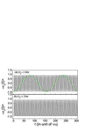
Figure 1: (Color online)The time-dependent quantum dynamics of $\left\langle\sigma_{z}(t)\right\rangle$ for the different driving magnitude $\Omega_{a}=1.2\omega$ (a) and $\Omega_{a}=1.25\omega$ (b) when $g=0.2\omega$ and $\varepsilon=0$.

With the time-independent driving field of photon, Hamiltonian (1) can be rewritten as $H_{P}=\omega a^{\dagger}a+\frac{1}{2}\varepsilon\sigma_{z}+g\sigma_{x}(a^{\dagger}+a)+\Omega_{p}(a^{\dagger}+a)$. We first consider the case of $\varepsilon=0$, in which the quantum dynamics of $\left\langle\sigma_{z}(t)\right\rangle$ can be solved exactly for a given initial state. In the following discussions, this initial state is chosen as the eigenstate of Hamiltonian $H_{P}$ without the external driving $(\Omega_{p}=0)$, namely, $H_{P}^{\Omega=0}=\omega a^{\dagger}a+g\sigma_{x}(a^{\dagger}+a)$. Apparently, Hamiltonian $H_{P}^{\Omega=0}$ has the property that $H_{P}^{\Omega=0}(-a^{\dagger},-a,-\sigma_{x})=H_{P}^{\Omega=0}(a^{\dagger},a,\sigma_{x})$, which gives rise to the degenerate ground states $\left|G_{\pm}(0)\right\rangle=\left|z_{\pm}(0)\right\rangle\otimes\left|\pm\right\rangle$, where $\left|z_{\pm}(0)\right\rangle=D(\mp\frac{g}{\omega})\left|0\right\rangle$ with $\left|0\right\rangle$ being the vacuum state of photon and $D(\xi)=\exp(\xi a^{\dagger}-\xi^{\ast}a)$ being the displacement operator, and $\left|\pm\right\rangle$ are the eigenstate of $\sigma_{x}$ Hwang .

After the external driving field of photon is applied to control the evolution of the coherent states, the degeneracy of Hamiltonian $H_{P}^{\Omega\neq 0}[=\omega a^{\dagger}a+g\sigma_{x}(a^{\dagger}+a)+\Omega_{p}(a^{\dagger}+a)]$ breaks down. However, it still has a conserved quantity $\sigma_{x}$, and correspondingly, its dynamics can be well discussed in two subspaces with $\sigma_{x}=\pm 1$, whose effective Hamiltonians are given respectively by $H_{\pm}=$ $\omega a^{\dagger}a+g_{\pm}(a^{\dagger}+a)$ with $g_{\pm}=g\pm\Omega_{p}$. Under the initial states $\left|G_{\pm}(0)\right\rangle$, the time-independent wavefunctions for Hamiltonians $H_{\pm}$ can be obtained exactly by

$$\left|\varphi_{\pm}(t)\right\rangle=e^{i[\frac{g_{\pm}^{2}}{\omega}t-\frac{\Omega_{p}g_{\pm}}{\omega}\sin(\omega t)]}\left|z_{\pm}(t)\right\rangle\otimes\left|\pm\right\rangle,$$ (2)

where the coherent states for any time is given by $\left|z_{\pm}(t)\right\rangle=D(-g_{\pm}/\omega+\Omega_{p}e^{-i\omega t})\left|0\right\rangle$. Based on these time-dependent wavefunctions $\left|\varphi_{\pm}(t)\right\rangle$, the total wavefunction for Hamiltonian $H_{P}^{\Omega\neq 0}$ is given by $\left|\psi(t)\right\rangle=\left|\varphi_{+}(t)\right\rangle-\left|\varphi_{-}(t)\right\rangle$, which leads to the required dynamics $\left\langle\sigma_{z}(t)\right\rangle=-\left\langle\varphi_{+}(t)\right|\sigma_{z}\left|\varphi_{-}(t)\right\rangle-\left\langle\varphi_{-}(t)\right|\sigma_{z}\left|\varphi_{+}(t)\right\rangle$ Note , namely,

$$\left\langle\sigma_{z}(t)\right\rangle=-\exp(-\frac{2g^{2}}{\omega^{2}})\cos[\eta t-\xi\sin(\omega t)],$$ (3)

where $\eta=4g\Omega_{p}/\omega$ and $\xi=4g\Omega_{p}/\omega^{2}$.

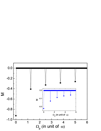
Figure 2: (Color online) The mean value $M$ of $\left\langle\sigma_{z}(t)\right\rangle$ for a long time $T_{L}=50\pi/\omega$ as a function of the driving amplitude $\Omega_{p}$ when $g=0.2\omega$ and $\varepsilon=0$. Insert: The initial state is chosen as the random state $\left|G(0)\right\rangle_{R}$.

Equation (3), which is the main result of this Letter, describes the quantum dynamics for any driving magnitude. It can be found that a coherent Rabi oscillation occurs here. Moreover, its period $T=\pi\omega/(2g\Omega_{p})$, unlike the traditional Rabi oscillation of the Jaynes-Cummings model, depends on the photon frequency $\omega$, the coupling strength $g$. In particular, this period is inversely proportional to the driving magnitude $\Omega_{p}$. If no driving is applied, this coherent Rabi oscillation disappears. However, the photon number wave packets can bounce back and forth along the same parity chains of Hamiltonian (1), while producing collapse and revivals of the initial population Casanova . In general, the term $\xi\sin(\omega t)$ has some effects on the time-dependent evolution of $\left\langle\sigma_{z}(t)\right\rangle$. In Fig. 1(a), the dynamics of $\left\langle\sigma_{z}(t)\right\rangle$ is plotted when $\Omega_{p}=1.2\omega$ and $g=0.2\omega$. In this figure, the dynamics depicted by the green line results from the influence of the term $\xi\sin(\omega t)$. However, in a special value for the strong driving magnitude, the dynamics is quite different. As shown in Fig. 1 (b), the green line disappears when $\Omega_{p}=1.25\omega$ with the same $g$. It seems that some exotic quantum effects occur in this strong driving. In order to show this clearly, we evaluate the mean value of $\left\langle\sigma_{z}(t)\right\rangle$ for a long time, namely, $M=\frac{1}{T_{L}}\int_{0}^{T_{L}}\left\langle\sigma_{z}(t)\right\rangle dt$.

Interestingly, by means of the first-kind Bessel function $B_{m}(a)$, the mean value $M$ is obtained by

$$M=-\exp(-\frac{2g^{2}}{\omega^{2}})B_{m}(m)f(\Omega_{p}^{m}),$$ (4)

where $f(\Omega_{p}^{m})$ is a jump function that satisfies $f(\Omega_{p}^{m})=1$ for $\Omega_{p}^{m}=m\omega^{2}/4g$ and $f(\Omega_{p}^{m})=0$ for $\Omega_{p}^{m}\neq m\omega^{2}/4g$. Figure 2 is plotted numerically the mean value $M$ for the time $T_{L}=50\pi/\omega$ as a function of the driving amplitude $\Omega_{p}$. It is shown in this figure that for a strong driving, namely, $\Omega_{p}^{m}=1.25m\omega$ ($g=0.2\omega$), a nonzero mean value $M$ can be found, whereas $M=0$ for $\Omega_{p}^{m}\neq 1.25m\omega$. This phenomenon exhibits clearly that a novel quantum resonant effect is predicted in the spin-boson model driven strongly by a photon field. Figure 2 also shows that at the different resonant position $\Omega_{p}^{m}=1.25\omega$, $2.5\omega$,$\cdots$, the magnitudes of the resonant peaks are different. Thus, it is very meaningful in experiment to implement a precise determination about the relative parameters by measuring $\Delta M_{m,m+i}=-\exp(-\frac{2g^{2}}{\omega^{2}})[B_{m+i}(m+i)-B_{m}(m)]$ with $i=1,2,\cdots$. For example, in terms of the measuable $\Delta M_{m,m+i}$, the couping strength can be obtained by

$$\frac{g}{\omega}=\sqrt{-\frac{1}{2}\ln\frac{\Delta M_{m,m+i}}{B_{m+i}(m+i)-B_{m}(m)}}.$$ (5)

On the other hand, based on the different resonant positions, the driving magnitude $\Omega_{p}$ can be also detected accurately. In the insert part of Fig. 2, we also check that, if the initial state is chosen as a random state $\left|G(0)\right\rangle_{R}=\sum_{N=0}^{N=5}(C_{N}^{+}\left|N,+\right\rangle+C_{N}^{-}\left|N,-\right\rangle)$, where $C_{N}^{\pm}=A_{\pm}\exp[i2\pi B_{\pm}]$ with $A_{\pm}$ and $B_{\pm}$ being two random numbers distributed in $[0,1)$ uniformly, the quantum resonant effect still remains at the same positions.

Figure 3: The mean value $M$ for a long time $T_{L}=50\pi/\omega$ as a function of the driving amplitude $\Omega_{p}$ when $g=0.2\omega$ and $\varepsilon=0.1\omega$. Insert: The quantum dynamics of $\left\langle\sigma_{z}(t)\right\rangle$ for $g=0.2\omega$, $\varepsilon=0.1\omega$ and $\Omega=1.25\omega$.

We now illustrate the physical explanation why this quantum resonant effect can occur. In term of the eigenstates $\left|\pm\right\rangle$ of $\sigma_{x}$, Hamiltonian $H_{P}$ with $\varepsilon=0$ has two subspaces, whose corresponding energies can be obtained exactly by $E_{\pm}=\omega N_{\pm}-g_{\pm}^{2}/\omega$ with $N_{\pm}$ being the photon numbers for $H_{\pm}$. Therefore, the gap between the branches of energy is given by $\Delta E_{\pm}=E_{+}-E_{-}=\omega m-4\Omega_{p}g/\omega$. For a weak driving, nothing happens in the gap $\Delta E_{\pm}$. However, for the strong driving, the gap becomes zero at the resonant positions $\Omega_{p}^{m}$. It means that the resonant effect perhaps has a correspondence on the crossing between two branches of energy. An important understanding of this resonant effect need to be analyzed the phase factors of the wavefunctions $\left|\varphi_{\pm}(t)\right\rangle$ in Eq. (2). These equations show clearly that the wavefunctions $\left|\varphi_{\pm}(t)\right\rangle$ have the nontrivial periodic phase factors $\alpha_{\pm}(t)=-\Omega_{p}g_{\pm}\sin\omega t/\omega$ apart from the dynamic phase factors $d_{\pm}(t)=g_{\pm}^{2}t/\omega$ when $\left|z_{\pm}(0)\right\rangle\rightarrow\left|z_{\pm}(t)\right\rangle$ driven by $H_{p}=\Omega_{p}(a^{\dagger}+a)$. When $t=2n\pi$ ($n=1,2,3,\cdots$), these periodic phase factors $\alpha_{\pm}(t)$ disappear, whereas the dynamic phase factors $d_{\pm}(t)$ still exist. Importantly, when calculating the quantum dynamics of $\left\langle\sigma_{z}(t)\right\rangle=-\left\langle\varphi_{+}(t)\right|\sigma_{z}\left|\varphi_{-}(t)\right\rangle-\left\langle\varphi_{-}(t)\right|\sigma_{z}\left|\varphi_{+}(t)\right\rangle$, these periodic phase factors in different subspaces generate a novel interference. As a result, the term $\xi\sin(\omega t)/2$ in Eq. (3) can be obtained. On the other hand, the nonorthogonal coherent states $\left\langle z_{+}(t)\right.\left|z_{-}(t)\right\rangle$ and $\left\langle z_{-}(t)\right.\left|z_{+}(t)\right\rangle$ with the complex parameters $\xi_{\pm}=-g_{\pm}/\omega+\Omega_{p}\exp(-i\omega t)$ also leads to another term $\xi\sin(\omega t)/2$ since $D(\xi_{+})D(\xi_{-})=D(\xi_{+}+\xi_{-})\exp[\frac{1}{2}(\xi_{+}\xi_{-}^{\ast}-\xi_{-}\xi_{+}^{\ast})]$.

Although the case $\varepsilon=0$ has been realized in the bichromatically excited of the trap ions Molmer and in the spin-orbit-coupled Bose-Einsten condensate with a harmonic trapped potential Lin1 , it is very necessary to discuss the case of $\varepsilon\neq 0$ in the cavity quantum electrodynamics. If the atomic resonant frequency $\varepsilon$ is taken into account, Hamiltonian $H_{P}$ is not integrable and the analytical dynamics, which is similar to Eq. (3), can not been derived. In Fig. 3, the quantum dynamics of $\left\langle\sigma_{z}(t)\right\rangle$ and its mean value $M$ for a long time are plotted numerically for $\varepsilon=0.1\omega$, whereas the other parameters are the same as those in Figs. (1) and (2). Due to the existence of the term $\varepsilon\sigma_{z}/2$, the quantum dynamics of $\left\langle\sigma_{z}(t)\right\rangle$ given in the insert part of Fig. 3 becomes more complicate. However, the quantum resonance effect with the same positions has still been manifest.

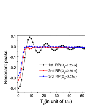
Figure 4: (Color online) The first (1st, $\Omega_{p}=1.25\omega$, black line), second (2nd, $\Omega_{p}=2.50\omega$, red line) and third (3d, $\Omega_{p}=3.75\omega$, blue line) resonant peaks (RPs) of the mean value $M$ for a long time $T_{L}=50\pi/\omega$ as a function of the rise time $T_{c}$ when $g=0.2\omega$ and $\varepsilon=0$.

Having obtained the fundamental properties of our predictions, we briefly address the possible observation in current experimental setup with the ultrastrong coupling. In principle, our predictions may be observed if the driving magnitude of the photon field is sufficiently large. As an example, we here consider the flux-based circuit quantum electrodynamics, in which the coupling strength $g=2\pi\times 314$ MHz has been reported for $\omega=2\pi\times 2.782$ GHz Niemczyk . This large coupling rate $(g/\omega\sim 0.11)$ allows us to enter the anticipant ultrastrong coupling regime. If using ratio $g/\omega=0.1$, the driving magnitudes for the resonant positions are given by $\Omega_{p}^{m}=2.5\omega$, $5.0\omega$,$\cdots$. With the increasing of the coupling strength in the near future, the required driving magnitues become weaker (for example, $\Omega_{p}^{m}=1.25\omega$, $2.5\omega$,$\cdots$ for $g/\omega=0.2$ in our calculations and $\Omega_{p}^{m}=0.5\omega$, $1.0\omega$,$\cdots$ for $g/\omega=0.5$). On the other hand, for the photon frequency $\omega=2\pi\times 2.782$ GHz, the integral time $T_{L}$ in Figs. (2) and (3) is given by $T_{L}=50\pi/\omega=$ $11$ ns, which are shorter than the decoherence time $t_{D}=1/\kappa=$ $64$ ns for $\kappa=2\pi\times 2.5$ MHz. It means that in the range of decoherence time, our predictions can be detected by measuring the excited state population MB . It should be pointed out that in all simulations above, the driving $H_{p}=\Omega_{p}(a^{\dagger}+a)$ is turned instantaneously on, which is a useful theoretical approximation. In fact, the resonant effect is very sensitive to the finite rise-time of the driving. In Fig. 4, we plot the first, second, and third resonant peaks of the mean value $M$ for the time $T_{L}=50\pi/\omega$ as a function of the rise time $T_{c}$, in which the driving magnitude is chosen as $\Omega(t)=t\Omega_{p}/T_{c}$ for $t<T_{c}$ and $\Omega(t)=\Omega_{p}$ for $t>T_{c}$. It can be found clearly in the figure that, if the rise time $T_{c}$ is long, the resonant effect can not be observed.

It is straightforward to find in quantum optics that the spin-boson model can be also driven by a time-independent field of atom $H_{a}=\Omega_{a}\sigma_{x}$ with $\Omega_{a}$ being the driving magnitude. In the strong coupling governed by the Jaynes-Cummings model, these drivings have almost the same effects on its dynamics. However, in the framework of the ultrastrong coupling, they generate quite different effects if their driving magnitudes are strong, as will be demonstated below. Without the atomic resonant level $(\varepsilon=0)$, the corresponding Hamiltonian is given by $H_{A}^{\varepsilon=0}=\omega a^{\dagger}a+g\sigma_{x}(a^{\dagger}+a)+\Omega_{a}\sigma_{x}$. Similar to Eq. (2), the wavefunctions for Hamiltonian $H_{A}^{\varepsilon=0}$ in the subspaces $\sigma_{x}=\pm 1$ is obtained, if the initial states is chosen as $\left|G_{\pm}(0)\right\rangle$, by $\left|\varphi_{\pm}(t)\right\rangle_{a}=e^{i(\frac{g^{2}}{\omega}t\pm\Omega_{a}t)}\left|z_{\pm}(0)\right\rangle\otimes\left|\pm\right\rangle$. In this wavefunctions, no periodic phase factor can be found. Moreover, the coherent states remain invariant with respect to $t$. Based on the wavefunctions $\left|\varphi_{\pm}(t)\right\rangle_{a}$, the quantum dynamics of $\left\langle\sigma_{z}(t)\right\rangle_{a}$ is also solved exactly by $\left\langle\sigma_{z}(t)\right\rangle_{a}=-\exp(-\frac{4g^{2}}{\omega})\cos(2\Omega_{a}t)$, which is quite different from Eq. (3) arising from the driving photon field. In this driving, the period of Rabi oscillation depends only on the driving magnitude $\Omega_{a}$. More importantly, no resonant effect can be found, even if the driving magnitude $\Omega_{a}$ is very strong.

In summery, simulated by the recent experiments of the solid-state quantum optics with the ultrastrong coupling, we have investigated the simple quantum dynamics to reveal the fundamental property of the spin-boson model, in which the counter-rotating terms must be considered. Our predications may be observed if the driving the photon field is sufficiently strong in experiments.

We thank Profs. J. -Q. Liang, Chuanwei Zhang, Jing Zhang, and Shiqun Zhu as well as Drs. Yongping Zhang, Jie Ma and Ming Gong for their helpful discussions and suggestions. This work was supported partly by the NNSFC under Grant Nos. 10904092, 10934004, 60978018, 11074184 and 11074154, and the ZJNSF under Grant No. Y6090001.

References

- (1) G. Günter, et. al., Nature (London) 458, 178 (2009).
- (2) A. A. Anappara, et. al., Phys. Rev. B 79, 201303 (2009).
- (3) Y. Todorov, et. al., Phys. Rev. Lett. 105, 196402 (2010).
- (4) A. Fedorov, et. al., Phys. Rev. Lett. 105, 060503 (2010).
- (5) T. Niemczyk, et. al., Nature Physics 6, 772 (2010).
- (6) J. Bourassa, et. al., Phys. Rev. A. 80, 032109 (2009).
- (7) B. Peropadre, P. Forn-Díaz, E. Solano, and J. J. García-Ripoll, Phys. Rev. Lett. 105, 023601 (2010).
- (8) E. T. Jaynes, and F.W. Cummings, Proc. IEEE 51, 89 (1963).
- (9) M. D. Crisp, Phys. Rev. A 43, 2430 (1991).
- (10) L. Lamata, J. León, T. Schätz, and E. Solano, Phys. Rev. Lett. 98, 253005 (2007).
- (11) H. Zheng, S. Y. Zhu, and M. S. Zubairy, Phys. Rev. Lett. 101, 200404 (2008).
- (12) R. Gerritsma, G. Kirchmair, F. Zähringer, E. Solano, R. Blatt, and C. F. Roos, Nature (London) 463, 68 (2009).
- (13) J. Larson, and S. Levin, Phys. Rev. Lett. 103, 013602 (2009).
- (14) J. Larson, Phys. Rev. A 81, 051803 (2010).
- (15) J. Hausinger, and M. Grifoni, Phys. Rev. A 83, 030301 (2011).
- (16) M. Hirokawa, arXiv: 1101.1770 (2011).
- (17) J. Casanova, G. Romero, I. Lizuain, J. J. García-Ripoll, and E. Solano, Phys. Rev. Lett. 105, 263603 (2010).
- (18) M. O. Scully, and M. S. Zubairy, Quantum Optics (Cambridge University Press, Cambridge, 1997).
- (19) J. M. Raimond, M. Brune, and S. Haroche, Rev. Mod. Phys. 73, 565 (2001).
- (20) R. J. Schoelkopf, and S. M. Girvin, Nature (London) 451, 664 (2008).
- (21) M. -J. Hwang, and M. -S. Choi, Phys. Rev. A 82, 025802 (2010).
- (22) For simplicity, the initial values and are chosen to be equal. For different initial values, only a phase factor is generated, and thus, the main results in this Letter are not affected.
- (23) K. Mølmer, and A. Sørensen, Phys. Rev. Lett. 82, 1835 (1999).
- (24) Y. -J. Lin, K. Jiménez-García, and I. B. Spielman, Nature (London) 471, 83 (2011).
- (25) M. Baur, et. al., Phys. Rev. Lett. 102, 243602 (2009).