Liouville-Arnold integrability of the pentagram map on closed polygons

Abstract

The pentagram map is a discrete dynamical system defined on the moduli space of polygons in the projective plane. This map has recently attracted a considerable interest, mostly because its connection to a number of different domains, such as: classical projective geometry, algebraic combinatorics, moduli spaces, cluster algebras and integrable systems.

Integrability of the pentagram map was conjectured in [16] and proved in [13] for a larger space of twisted polygons. In this paper, we prove the initial conjecture that the pentagram map is completely integrable on the moduli space of closed polygons. In the case of convex polygons in the real projective plane, this result implies the existence of a toric foliation on the moduli space. The leaves of the foliation carry affine structure and the dynamics of the pentagram map is quasi-periodic. Our proof is based on an invariant Poisson structure on the space of twisted polygons. We prove that the Hamiltonian vector fields corresponding to the monodoromy invariants preserve the space of closed polygons and define an invariant affine structure on the level surfaces of the monodromy invariants.

1 Introduction

The pentagram map is a geometric construction which carries one polygon to another. Given an $n$-gon $P$, the vertices of the image $T(P)$ under the pentagram map are the intersection points of consecutive shortest diagonals of $P$. The left side of Figure 1 shows the basic construction. The right hand side shows the second iterate of the pentagram map. The second iterate has the virtue that it acts in a canonical way on a labeled polygon, as indicated. The first iterate also acts on labeled polygons, but one must make a choice of labeling scheme; see Section 2.2. The simplest example of the pentagram map for pentagons was considered in [11]. In the case of arbitrary $n$, the map was introduced in [15] and further studied in [16, 17].

The pentagram map is defined on any polygon whose points are in general position, and also on some polygons whose points are not in general position. One sufficient condition for the pentagram map to be well defined is that every consecutive triple of points is not collinear. However, this last condition is not invariant under the pentagram map.

The pentagram map commutes with projective transformations and thereby induces a (generically defined) map

$$T:\mathcal{C}_{n}\to\mathcal{C}_{n}$$ (1.1)

where $\mathcal{C}_{n}$ is the moduli space of projective equivalence classes of $n$-gons in the projective plane. Mainly we are interested in the subspace $\mathcal{C}_{n}^{0}$ of projective classes convex $n$-gons. The pentagram map is entirely defined on $\mathcal{C}_{n}^{0}$ and preserves this subspace.

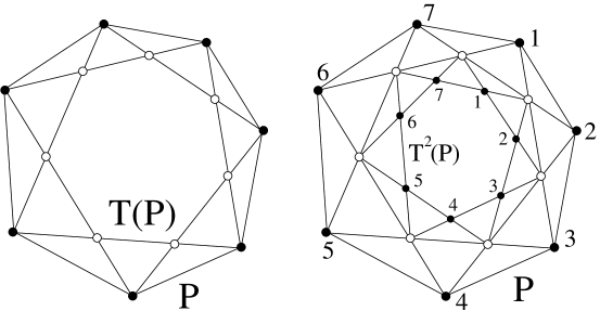
Figure 1: The pentagram map and its second iterate defined on a convex $7$-gon

Note that the pentagram map can be defined over an arbitrary field. Usually, we restrict our considerations to the geometrically natural real case of convex $n$-gons in ${\mathbb{RP}}^{2}$. However, the complex case represents a special interest since the moduli space of $n$-gons in ${\mathbb{CP}}^{2}$ is a higher analog of the moduli space $\mathcal{M}_{0,n}$. Unless specified, we will be using the general notation ${\mathbb{P}}^{2}$ for the projective plane and ${\mathrm{PGL}}_{3}$ for the group of projective transformations.

1.1 Integrability problem and known results

Assuming that the labeling schemes have been chosen carefully, the map $T:\mathcal{C}_{5}\to\mathcal{C}_{5}$ is the identity map and the map $T:\mathcal{C}_{6}\to\mathcal{C}_{6}$ is an involution. See [15]. The conjecture that the map (1.1) is completely integrable was formulated roughly in [15] and then more precisely in [16]. This conjecture was inspired by computer experiments in the case $n=7$. Figure 2 presents (a two-dimensional projection of) an orbit of a convex heptagon in ${\mathbb{RP}}^{2}$.

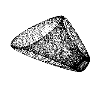
Figure 2: An orbit of the pentagram map on a heptagon

The first results regarding the integrability of the pentagram map were proved for the pentagram map defined on a larger space, ${\mathcal{P}}_{n}$, of twisted $n$-gons. A series of $T$-invariant functions (or first integrals) called the monodromy invariants, was constructed in [17]. In [13] (see also [12] for a short version), the complete integrability of $T$ on ${\mathcal{P}}_{n}$ was proved with the help of a $T$-invariant Poisson structure, such that the monodromy invariants Poisson-commute.

In [20], F. Soloviev found a Lax representation of the pentagram map and proved its algebraic-geometric integrability. The space of polygons (either ${\mathcal{P}}_{n}$ or $\mathcal{C}_{n}$) is parametrized in terms of a spectral curve with marked points and a divisor. The spectral curve is determined by the monodromy invariants, and the divisor corresponds to a point on a torus – the Jacobi variety of the spectral curve. These results allow one to construct explicit solutions formulas using Riemann theta functions (i.e., the variables that determine the polygon as explicit functions of time). Soloviev also deduces the invariant Poisson bracket of [13] from the Krichever-Phong universal formula.

Our result below has the same dynamical implications as that of Soloviev, in the case of real convex polygons. Soloviev’s approach is by way of algebraic integrability, and it has the advantage that it identifies the invariant tori explicitly as certain Jacobi varieties. Our proof is in the framework of Liuoville-Arnold integrability, and it is more direct and self-contained.

1.2 The main theorem

The main result of the present paper is to give a purely geometric proof of the following result.

Theorem 1.

Almost every point of $\mathcal{C}_{n}$ lies on a $T$-invariant algebraic submanifold of dimension

$$d=\left\{\begin{array}[]{l}n-4,\;n\;\hbox{is odd}\\ n-5,\;n\;\hbox{is even}.\end{array}\right.$$ (1.2)

that has a $T$-invariant affine structure.

Recall that an affine structure on a $d$-dimensional manifold is defined by a locally free action of the $d$-dimensional Abelian Lie algebra, that is, by $d$ commuting vector fields linearly independent at every point.

In the case of convex $n$-gons in the real projective plane, thanks to the compactness of the space established in [16], our result reads:

Corollary 1.1.

Almost every orbit in $\mathcal{C}^{0}_{n}$ lies on a finite union of smooth $d$-dimensional tori, where $d$ is as in equation (1.2). The union of these tori has a $T$-invariant affine structure.

Hence, the orbit of almost every convex $n$-gon undergoes quasi-periodic motion under the pentagram map. The above statement is precisely the integrability theorem in the Liouville–Arnold sense [1].

Let us also mention that the dimension of the invariant sets given by (1.2) is precisely a half of the dimension of $\mathcal{C}_{n}$, provided $n$ is odd, which is a usual, generic, situation for an integrable system. If $n$ is even, then $d=\frac{1}{2}\dim\mathcal{C}_{n}-1$ so that one can talk of “hyper-integrability”.

Our approach is based on the results of [17] and [13]. We prove that the level sets of the monodromy invariants on the subspace $\mathcal{C}_{n}\subset{\mathcal{P}}_{n}$ are algebraic subvarieties of $\mathcal{C}_{n}$ of dimension (1.2). We then prove that the Hamiltonian vector fields corresponding to the invariant functions are tangent to $\mathcal{C}_{n}$ (and therefore to the level sets). Finally, we prove that the Hamiltonian vector fields define an affine structure on a generic level set. The main calculation, which establishes the needed independence of the monodromy invariants and their Hamiltonian vector fields, uses a trick that is similar in spirit to tropical algebra.

One point that is worth emphasizing is that our proof does not actually produce a symplectic (or Poisson) structure on the space ${\cal C\/}_{n}$. Rather, we use the Poisson structure on the ambient space ${\mathcal{P}}^{n}$, together with the invariants, to produce enough commuting flows on ${\cal C\/}_{n}$ in order to fill out the level sets.

1.3 Related topics

The pentagram map is a particular example of a discrete integrable system. The main motivation for studying this map is its relations to different subjects, such as: a) projective differential geometry; b) classical integrable systems and symplectic geometry; c) cluster algebras; d) algebraic combinatorics of Coxeter frieze patterns. All these relations may be beneficial not only for the study of the pentagram map, but also for the above mentioned subjects. Let us mention here some recent developments involving the pentagram map.

• The relation of $T$ to the classical Boussinesq equation was essential for [13]. In particular, the Poisson bracket was obtained as a discretization of the (first) Adler-Gelfand-Dickey bracket related to the Boussinesq equation. We refer to [21, 22] and references therein for more information about different versions of the discrete Boussinesq equation.

• In [18], surprising results of elementary projective geometry are obtained in terms of the pentagram map, its iterations and generalizations.

• In [19], special relations amongst the monodromy invariants are established for polygons that are inscribed into a conic.

• In [2], the pentagram map is related to Lie-Poisson loop groups.

• The paper [8] concerns discretizations of Adler-Gelfand-Dickey flows as multi-dimensional generalizations of the pentagram map.

• A particularly interesting feature of the pentagram map is its relation to the theory of cluster algebras developed by Fomin and Zelevinsky, see [3]. This relation was noticed in [13] and developed in [6], where the pentagram map on the space of twisted $n$-gons is interpreted as a sequence of cluster algebra mutations, and an explicit formula for the iterations of $T$ is calculated.

• The structure of cluster manifold on the space $\mathcal{C}_{n}$ and the related notion of $2$-frieze pattern are investigated in [10].

2 Integrability on the space of twisted $n$-gons

In this section, we explain the proof of the main result in our paper [13], the Liouville-Arnold integrability of the pentagram map on the space of twisted $n$-gons. While we omit some technical details, we take the opportunity to fill a gap in [13]: there we claimed that the monodromy invariants Poisson commute, but our proof there had a flaw. Here we present a correct proof of this fact.

2.1 The space ${\mathcal{P}}_{n}$

We recall the definition of the space of twisted $n$-gons.

A twisted $n$-gon is a map $\phi:{\mathbb{Z}}\to{\mathbb{P}}^{2}$ such that

$$v_{i+n}=M\circ v_{i},$$ (2.3)

for all $i\in{\mathbb{Z}}$ and some fixed element $M\in{\mathrm{PGL}}_{3}$ called the monodromy. We denote by ${\mathcal{P}}_{n}$ the space of twisted $n$-gons modulo projective equivalence. The pentagram map extends to a generically defined map $T:{\mathcal{P}}_{n}\to{\mathcal{P}}_{n}$. The same geometric definition given for ordinary polygons works here (generically) and commutes with projective transformations.

In the next section we will describe coordinates on ${\mathcal{P}}_{n}$. These coordinates identify ${\mathcal{P}}_{n}$ as an open dense subset of ${\mathbb{R}}^{2n}$. Sometimes we will simply identify ${\mathcal{P}}^{n}$ with ${\mathbb{R}}^{2n}$. The space $\mathcal{C}_{n}$ is much more complicated; it is an open dense subset of a codimension $8$ subvariety of ${\mathbb{R}}^{2n}$.

Remark 2.1.

If $n\not=3m$, then it seems useful to impose the simple condition that $v_{i},v_{i+1},v_{i+2}$ are in general position for all $i$. With this condition, ${\mathcal{P}}_{n}$ is isomorphic to the space of difference equations of the form

$$V_{i}=a_{i}\,V_{i-1}-b_{i}\,V_{i-2}+V_{i-3},$$ (2.4)

where $a_{i},b_{i}\in{\mathbb{C}}$ or ${\mathbb{R}}$ are $n$-periodic: $a_{i+n}=a_{i}$ and $b_{i+n}=b_{i}$, for all $i$. Therefore, ${\mathcal{P}}_{n}$ is just a $2n$-dimensional vector space, provided $n\not=3m$. Let us also mention that the spectral theory of difference operators of type (2.4) is a classical domain (see [7] and references therein).

2.2 The corner coordinates

Following [17], we define local coordinates $(x_{1},\ldots,x_{2n})$ on the space ${\mathcal{P}}_{n}$ and give the explicit formula for the pentagram map.

Recall that the (inverse) cross ratio of $4$ collinear points in ${\mathbb{P}}^{2}$ is given by

$$[t_{1},t_{2},t_{3},t_{4}]=\frac{(t_{1}-t_{2})\,(t_{3}-t_{4})}{(t_{1}-t_{3})\,(t_{2}-t_{4})},$$ (2.5)

where $t$ is (an arbitrary) affine parameter.

Figure 3: Definition of the corned invariants

We define

$$\begin{array}[]{rcl}x_{2i-1}&=&\displaystyle\left[v_{i-2},\,v_{i-1},\,\left((v_{i-2},v_{i-1})\cap(v_{i},v_{i+1})\right),\,\left((v_{i-2},v_{i-1})\cap(v_{i+1},v_{i+2})\right)\right]\\[10.0pt] x_{2i+0}&=&\displaystyle\left[v_{i+2},\,v_{i+1},\,\left((v_{i+2},v_{i+1})\cap(v_{i},v_{i-1})\right),\,\left((v_{i+2},v_{i+1})\cap(v_{i-1},v_{i-2})\right)\right]\\[10.0pt] \end{array}$$ (2.6)

where $(v,w)$ stands for the line through $v,w\in{\mathbb{P}}^{2}$, see Figure 3. The functions $(x_{1},\ldots,x_{2n})$ are cyclically ordered: $x_{i+2n}=x_{i}$. They provide a system of local coordinates on the space ${\mathcal{P}}_{n}$ called the corner invariants, cf. [17].

Remark 2.2.

a) The index $2i+0$ just means $2i$. The zero is present to align the equations.

b) The right hand side of the second equation is obtained from the right hand side of the first equation just by swapping the roles played by $(+)$ and $(-)$. In light of this fact, it might seem more natural to label the variables so that the second equation defines $x_{2i+1}$ rather than $x_{2i+0}$. The corner invariants would then be indexed by odd integers. In Section 5 we will present an alternate labelling scheme which makes the indices work out better.

c) Continuing in the same vein, we remark that there are two useful ways to label the corner invariants. In [17] one uses the variables $x_{1},x_{2},x_{3},x_{4},...$ whereas in [13, 19] one uses the variables $x_{1},y_{1},x_{2},y_{2},...$. The explicit correspondence between the two labeling schemes is $x_{2i-1}\to{}x_{i},\,x_{2i}\to{}y_{i}$. We call the former convention the flag convention whereas we call the latter convention the vertex convention. The reason for the names is that the variables $x_{1},x_{2},x_{3},x_{4}$ naturally correspond to the flags of a polygon, as we will see in Section 5. The variables $x_{i},y_{i}$ correspond to the two flags incident to the $i$th vertex.

Let us give an explicit formula for the pentagram map in the corner coordinates. Following [13], we will choose the right labelling of the vertices of $T(P)$, see Figure 4. One then has (see [17]):

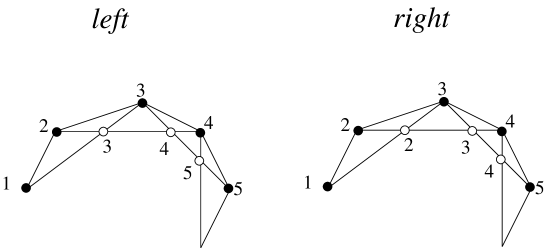
Figure 4: Left and right labelling

$$T^{*}x_{2i-1}=x_{2i-1}\,\frac{1-x_{2i-3}\,x_{2i-2}}{1-x_{2i+1}\,x_{2i+2}},\qquad T^{*}x_{2i}=x_{2i+2}\,\frac{1-x_{2i+3}\,x_{2i+4}}{1-x_{2i-1}\,x_{2i}},$$ (2.7)

where $T^{*}x_{i}$ stands for the pull-back of the coordinate functions.

2.3 Rescaling and the spectral parameter

Equation (2.7) has an immediate consequence: a scaling symmetry of the pentagram map.

Consider a one-parameter group ${\mathbb{R}}^{*}$ (or ${\mathbb{C}}^{*}$ in the complex case) acting on the space ${\mathcal{P}}_{n}$ multiplying the coordinates by $s$ or $s^{-1}$ according to parity:

$$\textstyle R_{t}:\,(x_{1},x_{2},x_{3}\ldots,x_{2n})\to(s\,x_{1},\,s^{-1}\,x_{2},\,s\,x_{3},\,\ldots,\,s^{-1}x_{2n}).$$ (2.8)

It follows from (2.7), that the pentagram map commutes with the rescaling operation.

We will call the parameter $s$ of the rescaling symmetry the spectral parameter since it defines a one-parameter deformation of the monodromy, $M_{s}$. Note that the notion of spectral parameter is extremely useful in the theory of integrable systems.

2.4 The Poisson bracket

Recall that a Poisson bracket on a manifold is a Lie bracket $\{.,.\}$ on the space of functions satisfying the Leibniz rule:

$$\{F,GH\}=\{F,G\}H+G\{F,H\},$$

for all functions $F,G$ and $H$. The Poisson bracket is an essential ingredient of the Liouville-Arnold integrability [1].

Define the following Poisson structure on ${\mathcal{P}}_{n}$. For the coordinate functions we set

$$\{x_{i},\,x_{i+2}\}=(-1)^{i}\,x_{i}\,x_{i+2},$$ (2.9)

and all other brackets vanish. In other words, the Poisson bracket $\{x_{i},x_{j}\}$ of two coordinate functions is different from zero if and only if $|i-j|=2$. The Leibniz rule then allows one to extend the Poisson bracket to all polynomial (and rational) functions.

Note that the Jacobi identity obviously holds. Indeed, the bracket (2.9) has constant coefficients when considered in the logarithmic coordinates $\log{}x_{i}$.

Proposition 2.3.

The pentagram map preserves the Poisson bracket (2.9).

Proof.

This is an easy consequence of formula (2.7), see [13] (Lemma 2.9), for the details. $\Box$

Recall that a Poisson structure is a way to associate a vector field to a function. Given a function $f$ on ${\mathcal{P}}_{n}$, the corresponding vector field $X_{f}$ is called the Hamiltonian vector field defined by $X_{f}(g)=\{f,g\}$ for every function $g$. In the case of the bracket (2.9), the explicit formula is as follows:

$$X_{f}=\sum_{i-j=2}(-1)^{\frac{i+j}{2}}\,\,x_{i}\,x_{j}\left(\frac{\partial{}f}{\partial{}x_{i}}\,\frac{\partial}{\partial{}x_{j}}-\frac{\partial{}f}{\partial{}x_{j}}\,\frac{\partial}{\partial{}x_{i}}\right).$$ (2.10)

Note that the definitions of the Poisson structure in terms of the bracket of coordinate functions (2.9) and in terms of the Hamiltonian vector fields (2.10) are equivalent.

Geometrically speaking, Hamiltonian vector fields are defined as the image of the map

$$X:T^{*}_{x}\,{\mathcal{P}}_{n}\to{}T_{x}\,{\mathcal{P}}_{n}$$ (2.11)

at arbitrary point $x\in{\mathcal{P}}_{n}$. The kernel of $X$ at a generic point is spanned by the differentials of the Casimir functions, that is, the functions that Poisson commute with all functions.

Remark 2.4.

The cluster algebra approach of [6] also provides a Poisson bracket, invariant with respect to the pentagram map (see the book [5]). It can be checked that this cluster Poisson bracket is induced by the bracket (2.9).

2.5 The rank of the Poisson bracket and the Casimir functions

The corank of a Poisson structure is the dimension of the kernel of the map $X$ in (2.11), that is, the dimension of the space generated by the differentials of the Casimir functions.

Proposition 2.5.

The Poisson bracket (2.9) has corank $2$ if $n$ is odd and corank $4$ is $n$ is even; the functions

$$O_{n}=x_{1}x_{3}\cdots{}x_{2n-1},\qquad E_{n}=x_{2}x_{4}\cdots{}x_{2n}$$ (2.12)

for arbitrary $n$ and the functions

$$O_{\frac{n}{2}}=\prod_{1\leq{}i\leq\frac{n}{2}}x_{4i-1}+\prod_{1\leq{}i\leq\frac{n}{2}}x_{4i+1},\qquad E_{\frac{n}{2}}=\prod_{1\leq{}i\leq\frac{n}{2}}x_{4i}+\prod_{1\leq{}i\leq\frac{n}{2}}x_{4i+2},$$ (2.13)

for even $n$, are the Casimirs of the Poisson bracket (2.9).

Proof.

First, one checks that the functions (2.12) and (2.13) are indeed Casimir functions (for arbitrary $n$ and for even $n$, respectively). To this end, it suffices to consider the brackets of (2.12) and (2.13), if $n$ is even, with the coordinate functions $x_{i}$.

Second, one checks that the corank of the Poisson bracket is equal to $2$, for odd $n$ and $4$, for even $n$. The corank is easily calculated in the coordinates $\log{}x_{i}$, see [13], Section 2.6 for the details. $\Box$

It follows that the Casimir functions are of the form $F\left(O_{n},E_{n}\right)$, if $n$ is odd, and of the form $F(O_{n/2},E_{n/2},O_{n},E_{n})$, if $n$ is even. In both cases the generic symplectic leaves of the Poisson structure have dimension $4[(n-1)/2]$.

Remark 2.6.

If $n$ is even, then the Casimir functions can be written in a more simple manner:

$$\Big{\{}\prod_{1\leq{}i\leq\frac{n}{2}}x_{4i-1},\quad\prod_{1\leq{}i\leq\frac{n}{2}}x_{4i+1},\quad\prod_{1\leq{}i\leq\frac{n}{2}}x_{4i},\quad\prod_{1\leq{}i\leq\frac{n}{2}}x_{4i+2}\Big{\}}$$

instead of (2.12) and (2.13).

2.6 Two constructions of the monodromy invariants

The second main ingredient of the Liouville-Arnold theory is a set of Poisson-commuting invariant functions. In this section, we recall the construction [17] of a set of first integrals of the pentagram map

$$O_{1},\ldots,O_{\left[\frac{n}{2}\right]},O_{n},\;E_{1},\ldots,E_{\left[\frac{n}{2}\right]},E_{n}$$

called the monodromy invariants. In other words, we will define $n+1$ invariant function on ${\mathcal{P}}_{n}$, if $n$ is odd, and $n+2$ invariant function on ${\mathcal{P}}_{n}$, if $n$ is even. The monodromy invariants are polynomial in the coordinates (2.6). Algebraic independence of these polynomials was proved in [17]. Note that $O_{n}$ and $E_{n}$ are the Casimir functions (2.12) and, for even $n$, the functions $O_{\frac{n}{2}}$ and $E_{\frac{n}{2}}$ are as in (2.13).

The indexing of the function $O_{i},E_{j}$ corresponds to their weight. More precisely, we define the weight of the coordinate functions by

$$\left|x_{2i+1}\right|=1,\qquad\left|x_{2i}\right|=-1.$$ (2.14)

Then, $|O_{k}|=k$ and $|E_{k}|=-k$. We give two definitions of the monodromy invariants. In [17] it is proved that the two definitions are equivalent.

A. The geometric definition. Given a twisted $n$-gon (2.3), the corresponding monodromy has a unique lift to ${\mathrm{SL}}_{3}$. By slightly abusing notation, we again denote this matrix by $M$. The two traces, $\mathrm{tr}(M)$ and $\mathrm{tr}(M^{-1})$, are preserved by the pentagram map (this is a consequence of the projective invariance of $T$). These traces are rational functions in the corner invariants. Consider the following two functions:

$$\widetilde{\Omega}_{1}=\mathrm{tr}(M)\,O_{n}^{\frac{2}{3}}\,E_{n}^{\frac{1}{3}},\qquad\widetilde{\Omega}_{2}=\mathrm{tr}(M^{-1})\,O_{n}^{\frac{1}{3}}\,E_{n}^{\frac{2}{3}}.$$

It turns out that $\widetilde{\Omega}_{1}$ and $\widetilde{\Omega}_{2}$ are polynomials in the corner invariants (see [17]). Since the pentagram map preserves the monodromy, and $O_{n}$ and $E_{n}$ are invariants, the two functions $\widetilde{\Omega}_{1}$ and $\widetilde{\Omega}_{2}$ are also invariants. We then have:

$$\widetilde{\Omega}_{1}=\sum_{k=0}^{[n/2]}O_{k},\qquad\widetilde{\Omega}_{2}=\sum_{k=0}^{[n/2]}E_{k},$$ (2.15)

where $O_{k}$ has weight $k$ and $E_{k}$ has weight $-k$ and where we set

$$O_{0}=E_{0}=1,$$

for the sake of convenience. The pentagram map preserves each homogeneous component individually because it commutes with the rescaling (2.8).

Notice also that, if $n$ is even, then $O_{\frac{n}{2}}$ and $E_{\frac{n}{2}}$ are precisely the Casimir functions (2.13). However, the invariants $O_{n}$ and $E_{n}$ do not enter the formula (2.15).

B. The combinatorial definition. Together with the coordinate functions $x_{i}$, we consider the following “elementary monomials”

$$X_{i}:=x_{i-1}\,x_{i}\,x_{i+1},\qquad i=1,\ldots,2n.$$ (2.16)

Let $O(X,x)$ be a monomial of the form

$$O=X_{i_{1}}\cdots{}X_{i_{s}}\,x_{j_{1}}\cdots{}x_{j_{t}},$$

where $i_{1},\ldots,i_{s}$ are even and $j_{1},\ldots,j_{t}$ are odd. Such a monomial is called admissible if the Poisson brackets $\{X_{i_{r}},X_{i_{u}}\}$ and $\{X_{i_{r}},x_{j_{u}}\}$ and $\{x_{j_{r}},x_{j_{u}}\}$ of all the elementary monomials entering $O$ vanish.

The weight of the above monomial is

$$|O|=s+t,$$

see (2.14). For every admissible monomial, we also define the sign of $O$ via

$$\mathrm{sign}(O):=(-1)^{t}.$$

The invariant $O_{k}$ is defined as the alternated sum of all the admissible monomials of weight $k$:

$$O_{k}=\sum_{|O|=k}\mathrm{sign}(O)\,O,\qquad k\in\left\{1,2,\ldots,\left[\frac{n}{2}\right]\right\}.$$ (2.17)

It is proved in [17] that this definition of $O_{k}$ coincides with (2.15).

Example 2.7.

The first two invariants are:

$$O_{1}=\sum_{i=1}^{n}\left(X_{2i}-x_{2i+1}\right),\qquad O_{2}=\sum_{|i-j|\geq 2}\left(x_{2i+1}\,x_{2j+1}-X_{2i}\,x_{2j+1}+X_{2i}\,X_{2j+2}\right),$$

for $n\leq 5$ the above formulas simplify, see [13].

The definition of the functions $E_{k}$ is exactly the same, except that the roles of even and odd are swapped.

Remark 2.8.

There is an elegant way to define the monodromy invariants in terms of determinants. See [19].

2.7 The monodromy invariants Poisson commute

In this section we give a complete proof of the following result, which was claimed in [13].

Theorem 2.

The monodromy invariants Poisson commute with each other, i.e.,

$$\{O_{i},O_{j}\}=\{O_{i},E_{j}\}=\{E_{i},E_{j}\}=0,$$

for all $i,j$ indexing the monodromy invariants. Hence, the Hamiltonian vector fields corresponding to the monodromy invariants $X_{O_{i}},\,X_{E_{i}}$ commute with each other.

Proof.

The second statement is a consequence of the first statement. So, we will just prove the first statement.

We begin with a prelimianry discussion of how the Poisson bracket interacts with the elementary monomials defined above. The Poisson brackets of elementary monomials

$$\left\{X_{i},X_{i+2}\right\}=(-1)^{i+1}\,X_{i}X_{i+2},\qquad\left\{X_{i},X_{i+4}\right\}=(-1)^{i+1}\,X_{i}X_{i+4},$$ (2.18)

together with

$$\left\{x_{i},X_{j}\right\}=\left\{\begin{array}[]{rl}(-1)^{i}\,x_{i}X_{j},&j=i+1,\,i+2,\,i+3,\\[8.0pt] (-1)^{i+1}\,x_{i}X_{j},&j=i-3,\,i-2,\,i-1,\end{array}\right.$$ (2.19)

immediately follow from the definition (2.9). All other brackets $\{X_{i},X_{j}\}$, as well as $\{X_{i},x_{j}\}$, vanish.

Now we are ready for the main argument. Consider first the Poisson bracket $\{O_{k},O_{m}\}$. This is a sum of the monomials of the form

$$m=X_{i_{1}}\cdots{}X_{i_{s}}x_{j_{1}}\cdots{}x_{j_{t}},$$

where $i_{1},\ldots,i_{s}$ are even and $j_{1},\ldots,j_{t}$ are odd. Indeed, by definition of the Poisson structure (2.9), the bracket of two monomials is proportional to their product, so that the above bracket contains only the monomials entering $O_{k}$ and $O_{m}$.

The monomial $m$ is not necessarily admissible. There can be squares (some $i$’s or $j$’s may coincide), but no cubes or higher degrees. We want to prove that the numeric coefficient of every such monomial in $\{O_{k},O_{m}\}$ is zero.

We define an oriented graph with the set of vertices $\{X_{i_{1}},\ldots,X_{i_{s}},\,x_{j_{1}},\ldots,x_{j_{t}}\}$ corresponding to the elementary monomials in $m$; the oriented arrows joining the vertices whenever their Poisson bracket is different from zero, the orientation being given by the sign of the bracket. Recall that all the non-zero brackets of elementary monomials are listed in (2.18) and (2.19).

Lemma 2.9.

If two indices coincide, $i_{r}=i_{u}$ or $j_{r}=j_{u}$, then the corresponding connected component of the graph consists of one element.

Proof.

If $i_{r}=i_{u}$, then $X_{i_{r}}=X_{i_{u}}$ belongs both to $O_{i}$ and $O_{j}$. By the admissibility condition, this implies all the Poisson brackets of $X_{i_{r}}$ with the other elementary monomials from $m$ vanish. $\Box$

The above lemma allows one to assume that all the indices in $m$ are different: $i_{r}\not=i_{u}$ and $j_{r}\not=j_{u}$.

Lemma 2.10.

The above defined graph has

(i) no $3$-cycles;

(ii) no vertices with more than one outgoing or ingoing arrows; in other words, the graph does not have the following vertices:

$$\begin{CD}\;@<{}<{}<a@>{}>{}>\;\qquad\;@>{}>{}>a@<{}<{}<\;\end{CD}$$

where $a=X_{i_{r}}$ or $x_{j_{u}}$.

Proof.

(i) Assume there is a $3$-cycle. Then at least two of the corresponding elementary monomials belong to the decomposition of either $O_{i}$ or $O_{j}$. The monomials are joined by an arrow, thus their Poisson bracket does not vanish. This leads to a contradiction since all the monomials in $O_{i}$ are admissible (see Section 2.6, definition B).

(ii) To show that no vertex of the graph can have more than one outgoing or ingoing arrows, one has to analyze formulas (2.18) and (2.19). Since $i_{r}$ are even and $j_{u}$ are odd, a vertex $X_{i_{r}}$ can be joined by an outgoing arrow to the following vertices (provided they belong to the graph): $X_{i_{r}-2},\,X_{i_{r}-4},\,x_{i_{r}+1},x_{i_{r}+3}$. In all of these cases, we obtain a 3-cycle, which is a contradiction to part (i) of the lemma. $\Box$

The above lemma implies the following statement.

Corollary 2.11.

The graph has no branching (i.e., vertices with three or more adjacent arrows).

Indeed, a branching point has more than one out- or ingoing arrows:

$$\begin{CD}@A{}A{}A\\ @>{}>{}>a@>{}>{}>\end{CD}\qquad\begin{CD}@A{}A{}A\\ @>{}>{}>a@<{}<{}<\end{CD}$$

Remark 2.12.

One can also show that the constructed graph has no $k$-cycles for arbitrary $k$, that is, every connected component of the graph is of type $A_{k}$ oriented in the standard way:

$$\begin{CD}a_{1}@>{}>{}>a_{2}@>{}>{}>\cdots @>{}>{}>a_{k}\end{CD}$$

but we will not use this in the proof.

Let us finally deduce $\{O_{i},O_{j}\}=0$ from Lemma 2.10 and Corollary 2.11. Every element $X_{i_{r}}$ and $x_{i_{u}}$ in the monomial $m$ belongs either to $O_{i}$, or to $O_{j}$. If the constructed graph contains at least three elements, then is has a fragment:

$$\begin{CD}a_{1}@>{}>{}>a_{2}@>{}>{}>a_{3}\end{CD}$$

where either $a_{1},a_{3}\in O_{i}$ and $a_{2}\in O_{j}$ or the other way around. It follows from the Leibniz identity that the element $a_{2}$ contributes twice in $\{O_{i},O_{j}\}$, namely in $\{a_{1},a_{2}\}$ and in $\{a_{3},a_{2}\}$, with the opposite signs.

We proved $\{O_{i},O_{j}\}=0$, except the case where the graph is of type $A_{2}$, i.e., contains only two elements:

$$\begin{CD}a_{1}@>{}>{}>a_{2}\end{CD}$$

with, say, $a_{1}\in O_{i},a_{2}\in O_{j}$. But in this last case, the Poisson brackets of the elementary monomials $a_{1}$ and $a_{2}$ with all the other elementary monomials in $m$ vanish. By construction of the invariants, $O_{i}$ and $O_{j}$ are symmetric with respect to the monomials $a_{1}$ and $a_{2}$. It follows that the monomial $m$ appears twice in $\{O_{i},O_{j}\}$, with the opposite signs. This completes the proof that $\{O_{i},O_{j}\}=0$.

The proof of $\{E_{i},E_{j}\}=0$ is identically the same (with odd and even indices exchanged). It remains to consider the bracket $\{O_{i},E_{j}\}$.

We will apply the same idea and construct a graph for every monomial in $\{O_{i},E_{j}\}$. Recall that $E_{j}$ contains the admissible monomials $E=X_{i_{1}}\cdots{}X_{i_{s}}\,x_{j_{1}}\cdots{}x_{j_{t}},$ where the indices $i_{1},\ldots,i_{s}$ are odd and $j_{1},\ldots,j_{t}$ are even. Analyzing the brackets (2.18) and (2.19), we see that the graph corresponding to any monomial in $\{O_{i},E_{j}\}$ is of the form

$$\setcounter{MaxMatrixCols}{11}\begin{CD}\cdots @>{}>{}>x_{i}@>{}>{}>X_{i+2}@>{}>{}>x_{i+4}@>{}>{}>X_{i+6}@>{}>{}>\cdots\end{CD}$$

and the $X$’s and $x$’s belong to the different functions. We observe that

$$\{x_{i},\,X_{i+2}\}=-\{X_{i+1},\,x_{i+3}\},$$

and if $x_{i}\in{}O_{i}$ and $X_{i+2}\in{}E_{j}$ then $O_{i}$ and $E_{j}$ are symmetric with respect to the exchange of $x_{i}$ with $X_{i+1}$ and of $X_{i+2}$ with $x_{i+3}$, respectively. The monomial $m$ appears twice with the opposite signs. This completes the proof of Theorem 2. $\Box$

In [17] it is proved that the monodromy invariants are algebraically independent. The argument is rather complicated, but it is very similar in spirit to the related independence proof we give in Section 4. The algebraic independence result combines with Theorem 2 to establish the integrability of the pentagram map on the space ${\mathcal{P}}_{n}$. Indeed, the Poisson bracket (2.9) defines a symplectic foliation on ${\mathcal{P}}_{n}$, the symplectic leaves being locally described as levels of the Casimir functions, see Proposition 2.5. The number of the remaining invariants is exactly half of the dimension of the symplectic leaves. The classical Liouville-Arnold theorem [1] is then applied.

3 Integrability on $\mathcal{C}_{n}$ modulo a calculation

The general plan of the proof of Theorem 1 is as follows.

1. We show that the Hamiltonian vector fields on ${\mathcal{P}}_{n}$ corresponding to the monodromy invariants are tangent to the subspace $\mathcal{C}_{n}$,

2. We restrict the monodromy invariants to $\mathcal{C}_{n}$ and show that the dimension of a generic level set is $n-4$ if $n$ is odd and $n-5$ if $n$ is even.

3. We show that there are exactly the same number of independent Hamiltonian vector fields.

In this section, we prove the first statement and also show that the dimension of the level sets is at most $n-4$ if $n$ is odd and $n-5$ if $n$ is even, and similarly for the number of independent Hamiltonian vector fields. The final step of the proof that this upper bound is actually the lower one will be done in the next two sections. This final step is a nontrivial calculation that comprises the bulk of the paper.

3.1 The Hamiltonian vector fields are tangent to $\mathcal{C}_{n}$

The space $\mathcal{C}_{n}$ is a subvariety of ${\mathcal{P}}_{n}$ having codimension $8$. It turns out that one can give explicit equations for this variety. See Lemma 5.3. (These equations do not play a role in our proof, but they are useful to have.)

The following statement is essentially a consequence of Theorem 2. This is an important step of the proof of Theorem 1.

Proposition 3.1.

The Hamiltonian vector field on ${\mathcal{P}}_{n}$ corresponding to a monodromy invariant is tangent to $\mathcal{C}_{n}$.

Proof.

The space ${\mathcal{P}}_{n}$ is foliated by isomonodromic submanifolds that are generically of codimension $2$ and are defined by the condition that the monodromy has fixed eigenvalues. Hence the isomonodromic submanifolds can be defined as the level surfaces of two functions, $\mathrm{tr}(M)$ and $\mathrm{tr}(M^{-1})$. This foliation is singular, and $\mathcal{C}_{n}$ is a singular leaf of codimension $8$. We note that the versal deformation of $\mathcal{C}_{n}$ is locally isomorphic to ${\mathrm{SL}}(3)$ partitioned into the conjugacy equivalence classes.

Consider a monodromy invariant, $F\,(=O_{i}$ or $E_{i}$), and its Hamiltonian vector field, $X_{F}$. We know that the Poisson bracket $\{F,\,\mathrm{tr}(M)\}=0$, since all monodromy invariants Poisson commute and $\mathrm{tr}(M)$ is a sum of monodromy invariants. Hence $X_{F}$ is tangent to the generic leaves of the isomonodromic foliation on ${\mathcal{P}}_{n}$. Let us show that $X_{F}$ is tangent to $\mathcal{C}_{n}$ as well.

In a nutshell, this follows from the observation that the tangent space to $\mathcal{C}_{n}$ at a smooth point $x_{0}$ is the intersection of the limiting positions of the tangent spaces to the isomonodromic leaves at points $x$ as $x$ tends to $x_{0}$. Assume then that $X_{F}$ is transverse to $\mathcal{C}_{n}$ at point $x_{0}\in\mathcal{C}_{n}$. Then $X_{F}$ will be also transverse to an isomonodromic leaf at some point $x$ close to $x_{0}$, yielding a contradiction.

More precisely, we can apply a projective transformation so that the vertices $V_{1},V_{2},V_{3},V_{4}$ of a twisted $n$-gon $V_{1},V_{2},\dots$ become the vertices of a standard square. This gives a local identification of ${\mathcal{P}}_{n}$ with the set of tuples $(V_{5},\dots,V_{n};M)$ where $M$ is the monodromy, the projective transformation that takes the quadruple $(V_{1},V_{2},V_{3},V_{4})$ to $(V_{n+1},V_{n+2},V_{n+3},V_{n+4}).$ The space of closed $n$-gons is characterized by the condition that $M$ is the identity. Thus we have locally identified ${\mathcal{P}}_{n}$ with $\mathcal{C}_{n}\times{\mathrm{SL}}(3)$. In particular, we have a projection ${\mathcal{P}}_{n}\to{\mathrm{SL}}(3)$, and the preimage of the identity is $\mathcal{C}_{n}$. The isomonodromic leaves project to the conjugacy equivalent classes in ${\mathrm{SL}}(3)$.

Thus our proof reduces to the following fact about the group ${\mathrm{SL}}(3)$ (which holds for ${\mathrm{SL}}(n)$ as well).

Lemma 3.2.

Consider the singular foliation of ${\mathrm{SL}}(3)$ by the conjugacy equivalence classes, and let $T_{X}$ be the tangent space to this foliation at $X\in{\mathrm{SL}}(3)$. Then the intersection, over all $X$, of the limiting positions of the spaces $T_{X}$, as $X\to 1\!\!1$, is trivial (here $1\!\!1\in{\mathrm{SL}}(3)$ is the identity).

Proof.

Let $B\in{\mathrm{SL}}(3)$, and let $B+\varepsilon C$ be an infinitesimal deformation within the conjugacy equivalence class. Then

$$\mathrm{tr}\left(B+\varepsilon C\right)=\mathrm{tr}(B),\qquad\mathrm{tr}\left((B+\varepsilon C)^{2}\right)=\mathrm{tr}\left(B^{2}\right),$$

hence $\mathrm{tr}(C)=0$ and $\mathrm{tr}(BC)=0$, and also $\mathrm{tr}(B^{-1}C)=0$ since $\det(B+\varepsilon C)=1$. Thus the tangent space to a conjugacy equivalent class of $B$ is given by

$$\mathrm{tr}(C)=\mathrm{tr}(BC)=\mathrm{tr}(B^{-1}C)=0.$$

Now let $B=1\!\!1+\varepsilon A$, a point in an infinitesimal neighborhood of the identity $1\!\!1$; we have $\mathrm{tr}(A)=0$. Then our conditions on $C$ implies $\mathrm{tr}(C)=\mathrm{tr}(AC)=0$. Since $\mathrm{tr}(AC)$ is a non-degenerate quadratic form, an element $C\in\mathrm{sl}(3)$ satisfying $\mathrm{tr}(AC)=0$ for all $A\in\mathrm{sl}(3)$ has to be zero. $\Box$

In view of what we said above, this implies the proposition. $\Box$

3.2 Identities between the monodromy invariants

In this section, we consider the restriction of the monodromy invariants from the space of all twisted $n$-gons to the space $\mathcal{C}_{n}$ of closed $n$-gons. We show that these restrictions satisfy 5 non-trivial relations, whereas their differentials, considered as covectors in ${\mathcal{P}}_{n}$ whose foot-points belong to $\mathcal{C}_{n}$, satisfy 3 non-trivial relations. These relations are also mentioned in [13] and [20]. In Sections 4 and 5, we will prove that there are no other relations between the monodromy invariants on $\mathcal{C}_{n}$ and their differentials along $\mathcal{C}_{n}$.

We remark that, strictly speaking, the identities established in this section are not needed for the proof of our main result. For the main result, all we need to know is that there are enough commuting flows to fill out what could be (a priori, with out the results in this section) a union of level sets of the monodromy invariants. Thus, the reader interested only in the main result can skip this section.

Theorem 3.

(i) The restrictions of the monodromy integrals to $\mathcal{C}_{n}$ satisfy the following five identities:

$$\begin{array}[]{rcl}\displaystyle\sum_{j=0}^{[n/2]}O_{j}=3\,E_{n}^{\frac{1}{3}}\,O_{n}^{\frac{2}{3}},&&\displaystyle\sum_{j=0}^{[n/2]}E_{j}=3\,E_{n}^{\frac{2}{3}}\,O_{n}^{\frac{1}{3}},\\[16.0pt] \displaystyle\sum_{j=1}^{[n/2]}j\,O_{j}=n\,E_{n}^{\frac{1}{3}}\,O_{n}^{\frac{2}{3}},&&\displaystyle\sum_{j=1}^{[n/2]}j\,E_{j}=n\,E_{n}^{\frac{2}{3}}\,O_{n}^{\frac{1}{3}},\\[16.0pt] \displaystyle E_{n}^{\frac{1}{3}}\,\sum_{j=1}^{[n/2]}j^{2}\,O_{j}&=&\displaystyle O_{n}^{\frac{1}{3}}\,\sum_{j=1}^{[n/2]}j^{2}\,E_{j}.\end{array}$$ (3.20)

(ii) The differentials of the monodromy integrals along $\mathcal{C}_{n}$ satisfy the three identities:

$$\begin{array}[]{rcl}\displaystyle\sum_{j=1}^{[n/2]}dO_{j}&=&\displaystyle 2\,E_{n}^{\frac{1}{3}}\,O_{n}^{-\frac{1}{3}}\,dO_{n}+E_{n}^{-\frac{2}{3}}\,O_{n}^{\frac{2}{3}}dE_{n},\\[16.0pt] \displaystyle\sum_{j=1}^{[n/2]}dE_{j}&=&\displaystyle 2\,E_{n}^{-\frac{1}{3}}\,O_{n}^{\frac{1}{3}}dE_{n}+E_{n}^{\frac{2}{3}}\,O_{n}^{-\frac{2}{3}}\,dO_{n},\\[16.0pt] \displaystyle O_{n}^{\frac{1}{3}}\,\Big{(}\sum_{j=1}^{[n/2]}j\ dE_{j}\Big{)}+E_{n}^{\frac{1}{3}}\,\Big{(}\sum_{j=1}^{[n/2]}j\ dO_{j}\Big{)}&=&\displaystyle n\,E_{n}^{\frac{2}{3}}O_{n}^{\frac{2}{3}}\left(E_{n}^{-1}dE_{n}+O_{n}^{-1}dO_{n}\right).\end{array}$$ (3.21)

Proof.

Recall that the monodromy invariants $O_{j}$ are the homogeneous components of the polynomial $O_{n}^{2/3}E_{n}^{1/3}\,\mathrm{tr}(M)$ with respect to the rescaling (2.8), where $s=e^{t}$ for convenience. Likewise, the monodromy invariants $E_{j}$ are homogeneous components of $O_{n}^{1/3}E_{n}^{2/3}\,\mathrm{tr}(M^{-1})$. Recall also that $O_{0}=E_{0}=1$.

Denote for simplicity $O_{n}^{1/3}E_{n}^{2/3}=U,\,O_{n}^{2/3}E_{n}^{1/3}=V$. Notice that the monodromy matrix $M$ has the unit determinant. Let $e^{\lambda_{1}},\ e^{\lambda_{2}},\ e^{\lambda_{2}}$ be the eigenvalues of $M$. One has

$$\lambda_{1}+\lambda_{2}+\lambda_{3}\equiv 0.$$ (3.22)

We consider a one-parameter family of $n$-gons depending on the rescaling parameter $t$, such that for $t=0$, the $n$-gon belongs to $\mathcal{C}_{n}$. The monodromy $M=M_{t}$ also depends on $t$ so that we think of $\lambda_{i}$ as functions of the corner coordinates $(x_{1},\ldots,x_{2n})$ and of $t$. For $t=0$, one has: $\lambda_{i}=0,\,i=1,2,3$ since $M_{0}=\mathrm{Id}$.

The eigenvalues of $M^{-1}$ are $e^{-\lambda_{1}},\ e^{-\lambda_{2}},\ e^{-\lambda_{2}}.$ Since the weights of $O_{i}$ and $E_{j}$ are $j$ and $-j$ respectively, the definition of the integrals writes as follows:

$$e^{\frac{nt}{3}}\,V\left(e^{\lambda_{1}}+e^{\lambda_{2}}+e^{\lambda_{2}}\right)=\sum_{j=0}^{[n/2]}e^{tj}\,O_{j},\qquad e^{-\frac{nt}{3}}\,U\left(e^{-\lambda_{1}}+e^{-\lambda_{2}}+e^{-\lambda_{2}}\right)=\sum_{j=0}^{[n/2]}e^{-tj}\,E_{j}.$$

which we rewrite as

$$V\left(e^{\lambda_{1}}+e^{\lambda_{2}}+e^{\lambda_{2}}\right)=\sum_{j=0}^{[n/2]}e^{t(j-\frac{n}{3})}\,O_{j},\qquad U\left(e^{-\lambda_{1}}+e^{-\lambda_{2}}+e^{-\lambda_{2}}\right)=\sum_{j=0}^{[n/2]}e^{-t(j-\frac{n}{3})}\,E_{j}.$$ (3.23)

Setting $t=0$ in these formulas yields the first two identities in (3.20). Next, differentiate these equations in $t$ :

$$V\,\sum_{i=1}^{3}\lambda_{i}^{\prime}\,e^{\lambda_{i}}=\sum_{j=0}^{[n/2]}\left(j-\frac{n}{3}\right)e^{tj}\,O_{j},$$

where $\lambda_{i}^{\prime}=d\lambda_{i}/dt$, and similarly for $E_{j}$. Set $t=0$, then the left-hand-side vanishes because $\sum\lambda_{i}^{\prime}=0$ due to (3.22). Hence

$$\sum_{j=0}^{[n/2]}j\,O_{j}=\frac{n}{3}\,\sum_{j=0}^{[n/2]}O_{j}=n\,V$$

due to the first identity in (3.20) and similarly for $E_{j}$. One thus obtains the third and the fourth identity in (3.20).

To obtain the fifth equation in (3.20), differentiate the equations (3.23) with respect to $t$ twice to get

$$\begin{array}[]{rcl}\displaystyle V\,\Big{(}\sum_{i=1}^{3}(\lambda_{i}^{\prime\prime}+\lambda_{i}^{\prime 2})\,e^{\lambda_{i}}\Big{)}&=&\displaystyle\sum_{j=0}^{[n/2]}\left(j-\frac{n}{3}\right)^{2}e^{tj}\,O_{j},\\[16.0pt] \displaystyle U\,\Big{(}\sum_{i=1}^{3}\left(-\lambda_{i}^{\prime\prime}+\lambda_{i}^{\prime 2}\right)\,e^{\lambda_{i}}\Big{)}&=&\displaystyle\sum_{j=0}^{[n/2]}\left(j-\frac{n}{3}\right)^{2}e^{-tj}\,E_{j}.\end{array}$$

Divide the first equality by $V$, the second by $U$, subtract one from another, and set $t=0$:

$$2\sum_{i=1}^{3}\lambda_{i}^{\prime\prime}=V^{-1}\sum_{j=0}^{[n/2]}\left(j-\frac{n}{3}\right)^{2}O_{j}-U^{-1}\sum_{j=0}^{[n/2]}\left(j-\frac{n}{3}\right)^{2}E_{j}.$$

The left hand side vanishes, due to (3.22), so

$$V^{-1}\,\sum_{j=0}^{[n/2]}\left(j-\frac{n}{3}\right)^{2}O_{j}=U^{-1}\,\sum_{j=0}^{[n/2]}\left(j-\frac{n}{3}\right)^{2}E_{j}.$$ (3.24)

Therefore

$$\begin{array}[]{l}\displaystyle V^{-1}\sum_{j=0}^{[n/2]}j^{2}\,O_{j}-\frac{2n}{3}\,V^{-1}\,\sum_{j=0}^{[n/2]}j\,O_{j}+V^{-1}\,\frac{n^{2}}{9}\,\sum_{j=0}^{[n/2]}O_{j}=\\[10.0pt] \displaystyle\hskip 56.9055ptU^{-1}\sum_{j=0}^{[n/2]}j^{2}\,E_{j}-\frac{2n}{3}\,U^{-1}\,\sum_{j=0}^{[n/2]}j\,E_{j}+U^{-1}\,\frac{n^{2}}{9}\,\sum_{j=0}^{[n/2]}E_{j}.\end{array}$$

The second and the third terms on the left and the right hand sides are pairwise equal, due to the first four identities in (3.20). This implies the fifth identity (3.20).

To prove (3.21), take differentials of (3.23):

$$\begin{array}[]{l}\displaystyle V\sum_{i=1}^{3}e^{\lambda_{i}}\,d\lambda_{i}+\Big{(}\sum_{i=1}^{3}e^{\lambda_{i}}\Big{)}\,dV=\\[10.0pt] \displaystyle\Big{(}\sum_{j=0}^{[n/2]}\left(j-\frac{n}{3}\right)e^{t(j-\frac{n}{3})}\,O_{j}\Big{)}dt+\sum_{j=0}^{[n/2]}e^{t(j-\frac{n}{3})}\,dO_{j},\end{array}$$

and

$$\begin{array}[]{l}\displaystyle-U\sum_{i=1}^{3}e^{-\lambda_{i}}\,d\lambda_{i}+\Big{(}\sum_{i=1}^{3}e^{-\lambda_{i}}\Big{)}\,dU=\\[10.0pt] \displaystyle-\Big{(}\sum_{j=0}^{[n/2]}\Big{(}j-\frac{n}{3}\Big{)}e^{-t(j-\frac{n}{3})}E_{j}\Big{)}\,dt+\sum_{j=0}^{[n/2]}e^{-t(j-\frac{n}{3})}\,dE_{j}.\end{array}$$

Set $t=0$: the first terms on the right hand sides vanish due to (3.22), and the first parentheses on the right hand sides vanish due to (3.20). We get

$$\sum_{j=0}^{[n/2]}dO_{j}=3\,dV,\qquad\sum_{j=0}^{[n/2]}dE_{j}=3\,dU,$$

the first two identities in (3.21).

Finally, differentiate the above equations with respect to $t$ and set $t=0$ to obtain:

$$\begin{array}[]{rcl}\displaystyle V\,\sum_{i=1}^{3}\lambda_{i}^{\prime}\,d\lambda_{i}+V\,\sum_{i=1}^{3}d(\lambda_{i}^{\prime})+\Big{(}\sum_{i=1}^{3}\lambda_{i}^{\prime}\Big{)}\,dV&=&\displaystyle\Big{(}\sum_{j=0}^{[n/2]}\left(j-\frac{n}{3}\right)^{2}O_{j}\Big{)}\,dt+\sum_{j=0}^{[n/2]}\left(j-\frac{n}{3}\right)dO_{j},\\[14.0pt] \displaystyle U\,\sum_{i=1}^{3}\lambda_{i}^{\prime}\,d\lambda_{i}-U\,\sum_{i=1}^{3}\,d(\lambda_{i}^{\prime})+\Big{(}\sum_{i=1}^{3}\lambda_{i}^{\prime}\Big{)}\,dU&=&\displaystyle\Big{(}\sum_{j=0}^{[n/2]}\left(j-\frac{n}{3}\right)^{2}E_{j}\Big{)}\,dt-\sum_{j=0}^{[n/2]}\left(j-\frac{n}{3}\right)dE_{j}.\end{array}$$

Once again, the second and the third sums on the left hand sides vanish, due to (3.22). Divide the first equation by $V$, the second by $U$, and subtract one from another, using (3.24):

$$V^{-1}\,\sum_{j=0}^{[n/2]}\left(j-\frac{n}{3}\right)dO_{j}+U^{-1}\,\sum_{j=0}^{[n/2]}\left(j-\frac{n}{3}\right)dE_{j}=0.$$

Hence

$$V^{-1}\,\sum_{j=0}^{[n/2]}j\,dO_{j}+U^{-1}\,\sum_{j=0}^{[n/2]}j\,dE_{j}=\frac{n}{3}\,\Big{(}V^{-1}\sum_{j=0}^{[n/2]}dO_{j}+U^{-1}\sum_{j=0}^{[n/2]}dE_{j}\Big{)}.$$

Due to the first two identities in (3.21), the right-hand-side equals $n\,(O_{n}^{-1}\,dO_{n}+E_{n}^{-1}\,dE_{n})$. This yields the third identity in (3.21). Theorem 3 is proved. $\Box$

Remark 3.3.

a) Let ${\cal E}$ be the Euler vector field that generates the scaling. Then

$${\cal E}(O_{j})=j\,O_{j},\qquad\ {\cal E}(E_{j})=-j\,E_{j}.$$

If one evaluates the differentials in the identities (3.21) on ${\cal E}$, one obtains the last three identities in (3.20). This is a check that (3.20) and (3.21) are consistent with each other.

b) Equivalently, (3.21) can be rewritten as

$$\begin{array}[]{rcl}\displaystyle 3\,dO_{n}&=&2\,E_{n}^{-\frac{1}{3}}\,O_{n}^{\frac{1}{3}}\,\Big{(}\sum_{j=1}^{[n/2]}dO_{j}\Big{)}-E_{n}^{-\frac{2}{3}}\,O_{n}^{\frac{2}{3}}\,\Big{(}\sum_{j=1}^{[n/2]}dE_{j}\Big{)},\\[16.0pt] \displaystyle 3\,dE_{n}&=&2\,E_{n}^{\frac{1}{3}}\,O_{n}^{-\frac{1}{3}}\,\Big{(}\sum_{j=1}^{[n/2]}dE_{j}\Big{)}-E_{n}^{\frac{2}{3}}\,O_{n}^{-\frac{2}{3}}\,\Big{(}\sum_{j=1}^{[n/2]}dO_{j}\Big{)},\\[12.0pt] 0&=&\displaystyle O_{n}^{\frac{1}{3}}\,\Big{(}3\sum_{j=1}^{[n/2]}j\ dE_{j}-n\sum_{j=1}^{[n/2]}dE_{j}\Big{)}+E_{n}^{\frac{1}{3}}\,\Big{(}3\sum_{j=1}^{[n/2]}j\,dO_{j}-n\sum_{j=1}^{[n/2]}dO_{j}\Big{)}.\end{array}$$

c) The identities (3.20) and (3.21) are satisfied in a larger subspace than $\mathcal{C}_{n}$, consisting of twisted polygons whose monodromy has equal eigenvalues. This subspace has codimension 2 in ${\mathcal{P}}_{n}$.

d) In both cases, $n$ odd and $n$ even, the kernel of the Poisson map $X$ (2.11) (spanned by the differentials of the Casimir functions) has zero intersection with the subspace of $T^{*}{\mathcal{P}}_{n}$ spanned by the relations 3.21.

3.3 Reducing the proof to a one-point computation

For ease of exposition, we will give our proof only in the odd case, and we set $n\geq 7$ odd. Modulo changing some of the indices, the even case is similar. We will explain everything in terms of the odd case and, at the end of this section, briefly explain what happens in the even case.

Let ${\cal M\/}$ denote the algebra generated by the monodromy invariants. In the Section 4 we make the following calculations.

1. There exist elements $F_{1},...,F_{n-2}\in\cal M$ and a point $p\in\mathcal{C}_{n}$ such that the differentials $dF,...,dF_{n-2}$ are linearly independent at $p$. Therefore, $dF,...,dF_{n-2}$ are linearly independent at almost all $q\in\mathcal{C}_{n}$.

2. There exists elements $G_{1},...,G_{n-4}\in\cal M$ and a point $p\in\mathcal{C}_{n}$ such that the differentials $dG_{1}|_{T_{p}\mathcal{C}_{n}},...,dG_{n-4}|_{T_{p}\mathcal{C}_{n}}$ are linearly independent. Therefore, $dG_{1}|_{T_{q}\mathcal{C}_{n}},...,dG_{n-4}|_{T_{q}\mathcal{C}_{n}}$ are linearly independent at almost all $q\in\mathcal{C}_{n}$.

In Calculation 1, we are computing the differentials on the ambient space ${\cal P\/}_{n}$ but evaluating them at a point of $\mathcal{C}_{n}$. In Calculation 2, we are computing the differentials on the ambient space, evaluating them at a point of $\mathcal{C}_{n}$, and restricting the resulting linear functionals to the tangent space of $\mathcal{C}_{n}$. In both calculations, we are actually evaluating at points in ${\mathbb{C}}_{n}^{0}$. In each case, what allows us to make a conclusion about generic points is that the monodromy invariants are algebraic.

Calculation 2 combines with Theorem 3 to show that there are exactly $n-4$ algebraically independent monodromy invariants, when restricted to $\mathcal{C}_{n}$. Hence, the generic common level set of the monodromy invariants $O_{i},E_{i}$, restricted to $\mathcal{C}_{n}$, has dimension $n-4$.

Next, we wish to prove that these level sets have locally free action of the abelian group ${\mathbb{R}}^{d}$ (or ${\mathbb{C}}^{d}$ in the complex case). For $F\in\cal M$, the Hamiltonian vector field $X_{F}$ is tangent to $\mathcal{C}_{n}$, by Proposition 3.1, and also tangent to the common level set of functions in $\cal M$. Finally, by Theorem 2, the Hamiltonian vector fields all commute with each other (i.e., define an action of the Abelian Lie algebra). The following lemma finishes our proof.

Lemma 3.4.

The Hamiltonian vector fields of the monodromy invariants generically span the monodromy level sets on $\mathcal{C}_{n}$.

Proof.

Let $\wedge^{1}{\mathcal{P}}_{n}$ denote the space of $1$-forms on ${\mathcal{P}}^{n}$. Let $\cal X$ denote the space of vector fields on $\mathcal{C}_{n}$. Let $d{\cal M\/}\subset\wedge^{1}{\mathcal{P}}_{n}$ denote the image of $\cal M$ under the $d$-operator. Calculation 1 shows that the vector space $d{\cal M\/}$ generically has dimension $n-2$ when evaluated at points of $\mathcal{C}^{n}$. At the same time, we have the Poisson map $X:d{\cal M\/}\to{\cal X\/}$, given by

$$X(dF)=X_{F},$$

see (2.11). In the odd case, the map $X$ has $2$ dimensional kernel, see Remark 3.3 d). Hence, $X$ has $n-4$ dimensional image, as desired. $\Box$

Now we explain explicitly how the results above give us the quasi-periodic motion in the case of closed convex polygons. We know from the work in [15] that the monodromy level sets on $\mathcal{C}_{n}^{0}$ are compact. By Sard’s Theorem, and by the calculations above, almost every level set is a smooth compact manifold of dimension $m=n-4$. By Sard’s Theorem again, and by the dimension count above, almost every level set $L$ possesses a framing by Hamiltonian vector fields. That is, there are $m$ Hamiltonian vector fields on $L$ which are linearly independent at each point and which define commuting flows. These vector fields define local coordinate charts from $L$ into ${\mathbb{R}}^{m}$, such that the overlap functions are translations. Therefore $L$ is a finite union of affine $m$-dimensional tori. The whole structure is invariant under the pentagram map, and so the pentagram map is a translation of $L$ relative to the affine structure on $L$. This is the quasi-periodic motion. Even more explicitly, some finite power of the pentagram map preserves each connected component of $L$ and is a constant shift on each connected component.

The Even Case: In the even case, we have the following calculations:

1. There exist elements $F_{1},...,F_{n-1}\in\cal M$ and a point $p\in\mathcal{C}_{n}$ such that the differentials $dF,...,dF_{n-1}$ are linearly independent at $p$. Therefore, $dF,...,dF_{n-1}$ are linearly independent at almost all $q\in\mathcal{C}_{n}$.

2. There exists elements $G_{1},...,G_{n-3}\in\cal M$ and a point $p\in\mathcal{C}_{n}$ such that the differentials $dG_{1}|_{T_{p}\mathcal{C}_{n}},...,dG_{n-3}|_{T_{p}\mathcal{C}_{n}}$ are linearly independent. Therefore, $dG_{1}|_{T_{p}\mathcal{C}_{n}},...,dG_{n-3}|_{T_{p}\mathcal{C}_{n}}$ are linearly independent at almost all $q\in\mathcal{C}_{n}$.

In this case, the common level sets generically have dimension $n-5$ and, again, the Hamiltonian vector fields generically span these level sets. The situation is summarized in the following table.

$$\begin{array}[]{c|c|c|c|}&\hfill{\rm Invariants}&\hfill{\rm Casimirs}&\hfill{\rm Level\ sets}\,/\,\hfill{\rm Hamiltonian}\,\hfill{\rm fields}\\ \cline{1-1}\cr\cline{2-2}\cr\cline{3-3}\cr\cline{4-4}\cr n\,\hfill{\rm odd}&n+1&2&d=n-4\\ \cline{1-1}\cr\cline{2-2}\cr\cline{3-3}\cr\cline{4-4}\cr n\,\hfill{\rm even}&n+2&4&d=n-5\\ \cline{1-1}\cr\cline{2-2}\cr\cline{3-3}\cr\cline{4-4}\cr\end{array}$$

4 The linear independence calculation

4.1 Overview

For any given (smallish) value of $n$, one can make the calculations directly, at a random point, and see that it works. The difficulty is that we need to make one calculation for each $n$. One might say that the idea behind our calculations is tropicalization. The monodromy invariants and their gradients are polynomials with an enormous number of terms. We only need to make our calculation at one point, but we will consider a $1$-parameter family of points, depending on a parameter $u$. As $u\to 0$, the different variables tend to $0$ at different rates. This sets up a kind of hierarchy (or filtration) on the the monomials comprising the polynomials of interest to us, and only the “heftiest” monomials in this hierarchy matter. This reduces the whole problem to a combinatorial exercise.

We take $n\geq 7$ odd. Let $m=(n-1)/2$. Recall that $\cal M$ is spanned by

$$O_{1},...,O_{m},O_{n},E_{1},...,E_{m},E_{n}.$$

We define

$$A_{k,\pm}=O_{k}\pm E_{k}.$$ (4.25)

For the first calculation, we use the monodromy invariants

$$A_{3,+},...,A_{m,+},A_{n,+},A_{2,-},...,A_{m,-},A_{n,-}.$$ (4.26)

For the second calculation, we use the monodromy invariants

$$A_{3,-},...,A_{m,-},A_{3,+},...,A_{m,+},A_{n,+}.$$ (4.27)

The point we use is of the form $p=P^{u}$, where $P^{u}$ is an $n$-gon having corner invariants

$$a,b,c,d,u^{1},u^{2},u^{3},u^{4},...,u^{4},u^{3},u^{2},u^{1},d,c,b,a,$$ (4.28)

Here

• $a=O(u^{(n-4)(n-3)/2})$.

• $b=1+O(u)$

• $c=1+O(u)$.

• $d=1+O(u)$.

We will show that the results hold when $u$ is sufficiently small. Here we are using the big O notation, so that $O(u)$ represents an expression that is at most $Cu$ in size, for a constant $C$ that does not depend on $u$.

We will construct $P^{u}$ in the next section. Our first calculation requires only the information presented above. The second calculation, which is almost exactly the same as the first calculation, requires some auxilliary justification. In order to justify the calculation we make, we need to make some estimates on the tangent space $T_{P^{u}}$ to $\mathcal{C}_{n}$ at $P^{u}$. We will also do this in the next section.

In Section 4.2 and Section 4.3 we will explain our two calculations in general terms. In Section 4.4 we will define the concept of the heft of a monomial, and we will use this concept to put a kind of ordering on the monomials that appear in the monodromy invariants of interest to us. Following the analysis of the heft, we complete the details of our calculations.

4.2 The first calculation in broad terms

Let $\nabla$ denote the gradient on ${\mathbb{R}}^{2n}$. Let $\widetilde{\nabla}$ denote the normalized gradient:

$$\widetilde{\nabla}F=\lambda^{-1}\nabla F;\hskip 30.0pt\lambda=\|\nabla F\|_{\infty}.$$ (4.29)

In practice, we never end up dividing by zero. So, the largest entry in $\widetilde{\nabla}F$ is $\pm 1$.

If $F$ is a monodromy invariant, the coordinates of $\widetilde{\nabla}F(P^{u})$ have a power series in $u$. We define $\Psi F$ to be the result of setting all terms except the constant term to $0$. We call $\Psi F$ the asymptotic gradient. Thus, if

$$\widetilde{\nabla}F(P^{u})=(1-u^{3}\cdots,-1+u\cdots,u^{2}\cdots,...)$$

then $\Psi F=(1,-1,0,...)$.

Lemma 4.1.

Suppose that $\Psi F_{1},...,\Psi F_{k}$ are linearly independent. Then likewise $\nabla F_{1},...,\nabla F_{k}$ are linearly independent at $P^{u}$ for $u$ sufficiently small. Equivalently, the same goes for $dF_{1},...,dF_{k}$.

Proof.

Since $\Psi F_{1},...,\Psi F_{k}$ are independent there is some $\epsilon>0$ such that a sum of the form

$$\bigg{|}\sum b_{j}\Psi F_{j}\bigg{|}<\epsilon;\hskip 30.0pt\max|b_{j}|=1$$

is impossible.

Suppose for the sake of contradiction that the gradients are linearly dependent at $P^{u}$ for all sufficiently small $u$. Then the normalized gradients are also linearly dependent at $P^{u}$ for all sufficiently small $u$. We may write

$$\sum b_{j}\widetilde{\nabla}F_{j}\cdot e_{i}=0;\hskip 30.0pt\max|b_{j}|=1.$$ (4.30)

for the standard basis vectors $e_{1},...,e_{2n}$. The coefficients $b_{j}$ possibly depend on $u$, but this doesn’t bother us.

We have the bound

$$\bigg{|}b_{j}\widetilde{\nabla}F_{j}-b_{j}\Psi F_{j}\bigg{|}=O(u).$$ (4.31)

Hence

$$\sum_{j}b_{j}\Psi F_{j}\cdot e_{i}=O(u)$$ (4.32)

for all basis vectors $e_{i}$. Therefore, we can take $u$ small enough so that

$$\bigg{|}\sum b_{j}\Psi F_{j}\bigg{|}<\epsilon;\hskip 30.0pt\max|b_{j}|=1,$$

in contradiction to what we said at the beginning of the proof. $\Box$

Remark 4.2.

The idea of the proof of the previous lemma is simple: given a matrix, algebraically dependent on a parameter $u$, the rank of the matrix is greatest in a Zariski open subset of the parameter space and can only drop for special values of the parameter (zero, in our case).

We form a matrix $M_{+}$ whose rows are $\Psi F$, where $F$ is each of the $A_{+}$ invariants. We similarly form the matrix $M_{-}$.

Lemma 4.3.

Each row of $M_{+}$ is orthogonal to each row of $M_{-}$.

Proof.

Consider the map $T:{\mathbb{R}}^{2n}\to{\mathbb{R}}^{2n}$ which simply reverses the coordinates. We have $E_{k}\circ T=O_{k}$ for all $k$ and moreover $T(P^{u})=P^{u}$. Letting $dT$ be the differential of $T$, we have

$$dT(\nabla A_{k,\pm})=\pm\nabla A_{k,\pm}.$$ (4.33)

Our lemma follows immediately from this equation, and from the fact that $T$ is an isometric involution. $\Box$

In view of Lemmas 4.1 and Lemma 4.3, our first calculation follows from the statements that $M_{+}$ and $M_{-}$ have full rank.

For the matrix $M_{+}$, we consider the minor $m_{+}$ consisting of columns

$$1,6,7,10,11,14,15,18,19,...$$

until we have a square matrix. We will prove below that $m_{+}$ has the following form (shown in the case $n=13$.)

$$\left[\begin{matrix}0&\pm 1&\pm 1&\pm 1&\pm 1\cr 0&0&\pm 1&\pm 1&\pm 1\cr 0&0&0&\pm 1&\pm 1\cr 0&0&0&0&\pm 1\cr\pm 1&0&0&0&0\end{matrix}\right]$$ (4.34)

This matrix always has full rank. Hence $M_{+}$ has full rank.

For the matrix $M_{-}$ we consider the minor $m_{-}$ consisting of columns

$$1,{\bf 3\/},6,7,10,11,14,15,18,19,...$$

The only difference here is that column $3$ is inserted. The resulting matrix has exactly the same structure as just described. Hence $M_{-}$ has full rank.

4.3 The second calculation in broad terms

Let $T=T_{P^{u}}(\mathcal{C}_{n})$ denote the tangent space to $\mathcal{C}_{n}$ at $P^{u}$. Let $\{e_{k}\}$ denote the standard basis for ${\mathbb{R}}^{2n}$. Let $\pi:{\mathbb{R}}^{2n}\to{\mathbb{R}}^{2n-8}$ denote the map which strips off the first and last $4$ coordinates.

Define

$$\nabla_{8}=\pi\circ\nabla.$$ (4.35)

We define the normalized version $\widetilde{\nabla}_{8}$ exactly as we defined $\widetilde{\nabla}$. Likewise we define $\Psi_{8}G$ for any monodromy function $G$.

For a collection of vectors $v_{5},\dots,v_{2n-4}$ to be specified in the next lemma, we form the vector

$$\Upsilon_{8}G=(D_{v_{5}}G,...,D_{v_{2n-4}}G)$$ (4.36)

made from the directional derivatives of $G$ along these vectors. Note, by way of analogy, that

$$\nabla_{8}G=(D_{e_{5}}G,...,D_{e_{2n-4}}G).$$ (4.37)

We define the normalized version $\widetilde{\Upsilon}_{8}$ exactly as we defined $\widetilde{\nabla}_{8}$.

In the next section, we will establish the following result.

Lemma 4.4 (Justification).

There is a basic $v_{5},...,v_{2n-4}$ for $T_{P^{u}}(\mathcal{C}_{n})$ such that $\pi(v_{k})=e_{k}$ for all $k$ and

$$\widetilde{\Upsilon}_{8}G-\widetilde{\nabla}_{8}G=O(u).$$

Corollary 4.5.

Suppose that $\Psi_{8}G_{1},...,\Psi_{8}G_{k}$ are linearly independent. Then the restrictions of $dG_{1},...,dG_{k}$ to $T_{P^{u}}(\mathcal{C}_{n})$ are linearly independent for $u$ sufficiently small.

Proof.

Given our basis, $\Psi_{8}$ represents the constant term approximation of both $\widetilde{\Upsilon}_{8}$ and $\widetilde{\nabla}_{8}$. So, the same proof as in Lemma 4.1 shows that the vectors $\widetilde{\Upsilon}_{8}G_{j}$ are linearly independent. This is equivalent to the conclusion of our corollary. $\Box$

Using the invariants listed in (4.27), we form the matrices $M_{+}$ and $M_{-}$ just as above, using $\Psi_{8}$ in place of $\Psi$. Lemma 4.3 again shows that each row of $M_{+}$ is orthogonal to each row of $M_{-}$. Hence, we can finish the second calculation by showing that both $M_{+}$ and $M_{-}$ have full rank.

For $M_{-}$ we create a square minor $m_{-}$ using the columns

$$2,3,6,7,10,11,14,15,...$$

Again, we continue until we have a square. It turns out that $m_{-}$ has the form

$$\left[\begin{matrix}\pm 1&\pm 1&\pm 1&\pm 1\cr 0&\pm 1&\pm 1&\pm 1\cr 0&0&\pm 1&\pm 1\cr 0&0&0&\pm 1\cr\end{matrix}\right]$$ (4.38)

Hence $M_{-}$ has full rank.

For $M_{+}$ we create a square minor $m_{+}$ using the same columns, but extending out one further (on account of the larger matrix size.) It turns out that $m_{+}$ has the same form as $m_{-}$. Hence $M_{+}$ has full rank.

4.4 The heft

Any monomial in the variables $x_{1},...,x_{2n}$, when evaluated at $P^{u}$, has a power series expansion in $u$. We define the heft of the monomial to be the smallest exponent that appears in this series. For instance, the heft of $u^{2}+u^{3}$ is $2$. We define the heft of a polynomial to be the minimum heft of the monomials that comprise it. Given a polynomial $F$, we define heft of $\nabla F$ to be the minimum heft, taken over all partial derivatives $\partial F/\partial x_{j}$.

We call a monomial term of $\partial F/\partial x_{k}$ hefty if its heft realizes the heft of $\nabla F$. We define $H_{k}F$ to be the sum of the hefty monomials in $\partial F/\partial x_{k}$. Each monomial occurs with sign $\pm 1$. We define $|H_{k}F|\in{\mathbb{Z}}$ to be the sum of the coefficients of the hefty terms in $H_{k}F$. We say that $F$ is good if $|H_{k}F|\not=0$ for at least one index $k$. If $F$ is good then

$$\Psi F=C(|H_{1}F|,...,|H_{2n}F|),$$ (4.39)

for some nonzero constant $C$ that depends on $F$. It turns out that $C=\pm 1$ in all cases.

We say that $F$ is great if $F$ is good and $|H_{k}F|\not=0$ for at least one index $k$ which is not amongst the first or last $4$ indices. When $F$ is great, not only does equation (4.39) hold, but we also have

$$\Psi_{8}F=C(|H_{5}F|,...,|H_{2n-4}F|),$$ (4.40)

Lemma 4.6.

Let $k=2,3$. Then $A_{k,\pm}$ is great and $\nabla A_{k,\pm}$ has heft $0$.

Proof.

Let $F=A_{k,\pm}$. Consider the case $k=2$. The argument turns out to be the same in the $(+)$ and $(-)$ cases. We say that an outer variable is one of the first or last $4$ variables in ${\mathbb{R}}^{2n}$, and we call the remaining variables inner. Since $x_{2}x_{6}$ and $x_{6}x_{2n-2}$ are both terms of $F$, we see that

$$H_{6}F=x_{2}+x_{2n-2}+...$$

In particular, $\nabla F$ has heft $0$. Any term in $H_{6}F$ involves only the outer $8$ variables, and a short case-by-case analysis shows that there are no other possibilities besides the two terms listed above. Hence $|H_{6}F|=2$. This shows that $F$ is great.

Now consider the case $k=3$. The argument turns out to be the same in the $(+)$ and $(-)$ cases. Since $x_{2}x_{6}x_{2n-2}$ is a term of $F$ we see that

$$H_{6}F=x_{2}x_{2n-2}+...$$

The rest of the proof is as in the previous case, with the only difference being that $|H_{6}F|=1$ in this case. $\Box$

From now on, we fix some $F=A_{k,\pm}$ with $3<k\leq m$. Let $\alpha_{1},\alpha_{2},...$ be the terms of the following sequence

$$0,0,0,2,3,6,7,10,11,14,15,...$$ (4.41)

Lemma 4.7.

$\nabla F$ has heft at most $\alpha_{1}+...+\alpha_{k}$.

Proof.

We describe a specific term in $\nabla F$ having heft $\alpha_{1}+...+\alpha_{k}$. We make a monomial using the indices

$$2,2n-2,6,2n-6,10,2n-10,...$$ (4.42)

stopping when we have used $k-1$ numbers. The monomial corresponding to these indices has heft

$$0+0+0+2+3+6+7+10+11...=\alpha_{1}+...+\alpha_{k}.$$

Thinking of our indices cyclically, we see that our integers lie in an interval of length $4k-7$. So, between the largest index in (4.42) that is less than $n$ and the smallest index greater than $n$ there is an unoccupied stretch of at least $9$ integers. The point here is that

$$9+(4k-7)\leq 9+4m-7=9+2(n-1)-7=2n.$$

Given that the unoccupied stretch has at least $9$ consecutive integers, there is at least $1$ (and in fact at least $2$) even indices $j$ such that the monomial

$$m=\pm x_{j}x_{2}x_{2n-2}x_{6}x_{2n-6}x_{10}...$$

is a term of $F$. But then $\partial m/\partial x_{j}$ has heft $\alpha_{1}+...+\alpha_{k}$. $\Box$

We mention that (4.42) is one of two obvious ways to make a term of heft $\alpha_{1}+...+\alpha_{k}$. The other way is to take the mirror image, namely

$$2n-1,3,2n-5,7,2n-9,11,...$$ (4.43)

Lemma 4.8.

If $\partial F/\partial x_{j}$ has a hefty term, then $j$ is an inner variable.

Proof.

For ease of exposition, we will consider the case when $j$ is one of the first $4$ variables. Let $(i_{1},...,i_{d})$ be the sequence of indices which appear in a term $m^{\prime}$ of $\partial F/\partial x_{j}$. The corresponding term $m$ in $F$ has index sequence $(j,i_{1},...,i_{d})$, where these numbers are not necessarily written in order. We know that at least one of the indices, say $a$, is an inner variable. By construction $\partial m/\partial x_{a}$ has smaller heft than $m^{\prime}$. Hence $\partial F/\partial x_{j}$ has no hefty terms. Hence $j$ is an inner variable. $\Box$

Lemma 4.9.

Suppose the monomial $\pm x_{i_{1}}...x_{i_{a}}$ is a hefty term of $\partial F/\partial x_{j}$. Then $a=k-1$ and $i_{1},...,i_{k-1}$ are either as in (4.42) or as in equation (4.43).

Proof.

We have to play the following game: We have a grid of $2n$ dots. The first and last dot are labelled $(n-3)(n-4)/2$. The remaining $6$ outer dots are labelled $0$. The inner dots are labelled $1,2,3,...,3,2,1$. Say that a block is a collection of $d$ dots in a row for $d=1,2,3$. We must pick out either $k$ or $k-1$ blocks in such a way that the total sum of the corresponding dots is as small as possible, and the (cyclically reckoned) spacing between consecutive blocks is at least $4$. That is, at least $3$ “unoccupied dots” must appear between every two blocks.

It is easy to see that one should use $k-1$ blocks, all having size $1$. Moreover, half (or half minus one) of the blocks should crowd as much as possible to the left and half minus one (or half) of the blocks should crowd as much as possible to the right. A short case by case analysis of the placement of the first and last blocks shows that one must have precisely the choices made in (4.42) and (4.43). $\Box$

Corollary 4.10.

Let $F=A_{k,\pm}$, with $k\geq 2$. Then $F$ is good. If $k\leq m$ then $F$ is great, and the heft of $\nabla F$ is $\alpha_{1}+...+\alpha_{k}$.

Proof.

In light of the results above, the only nontrivial result is that $F$ is great when $3<k\leq m$. The construction in connection with (4.42) produces a hefty term of $\partial F/\partial x_{j}$ for some inner index $j$. The key observation is that, for parity considerations, the mirror term corresponding to (4.43) is not a term of $\partial F/\partial x_{j}$. In one case $j$ must be odd and in the other case $j$ must be even. Hence, there is only $1$ hefty term in $\partial F/\partial x_{j}$. $\Box$

As regards the heft, we have done everything but analyze the Casimirs. Recall that

$$O_{n}=x_{1}x_{3}...x_{2n-1};\hskip 30.0ptE_{n}=x_{2}x_{4}...x_{2n}.$$ (4.44)

Lemma 4.11.

$A_{n,\pm}$ is good and $\nabla A_{n,+}$ has heft

$$\frac{(n-3)(n-4)}{2}.$$

Moreover,

$$\Psi A_{n,\pm}=(1,0,...,0,\pm 1).$$

Proof.

Let $F$ be either of these functions. Clearly the hefty terms of $\nabla F$ are the ones which omit the first and last variables. From here, this lemma is an exercise in arithmetic. $\Box$

A similar argument proves

Lemma 4.12.

$A_{n,\pm}$ is good and $\nabla_{8}A_{n,+}$ has heft $(n-4)^{2}$. Moreover,

$$\Psi A_{n,\pm}=(0,...,0,\pm 1,1,0,...,0),$$

with the $2$ middle indices being nonzero.

4.5 Completion of the first calculation

To complete the first calculation, we need to analyze the matrix made from the asymptotic gradients $\Psi F_{1},\Psi F_{2},...$. We deal with the first two in a calculational way.

Lemma 4.13.

$\Psi A_{2,\pm}=(0,0,\pm 1,0,0,1,\pm 1,...,1,\pm 1,0,0,1,0,0)$.

Proof.

Let $F=A_{2,\pm}$. We know that $F$ has heft $0$, so the hefty terms in $\nabla F$ are monomials which only involve the outer indices. Hence, when $8\leq j\leq 2n-8$ the result only depends on the parity of $j$ and neither the value of $j$ nor the value of $n$. For the remaining indices, the result is also independent of $n$. Thus, a calculation in the case (say) $n=13$ is general enough to rigorously establish the whole pattern. This is what we did. $\Box$

Lemma 4.14.

$\Psi A_{3,\pm}=(0,0,0,0,0,1,\pm 1,...,1,\pm 1,0,0,1,0,0)$.

Proof.

Same method as the previous result. $\Box$

Now we are ready to analyze the minors $m_{+}$ and $m_{-}$ described in connection with the first calculation. When we say that a certain part of one of these matrices has the form given by (4.34), we understand that (4.34) gives a smallish member of an infinite family of matrices, all having the same general type. So, we mean to take the corresponding member of this family which has the correct size.

We say that a given row or column of one of our matrices checks if it matches the form given by (4.34). We will give the argument for $m_{+}$. The case for $m_{-}$ is essentially the same.

Lemma 4.15.

The first column of $m_{+}$ checks.

Proof.

By Lemma 4.11, the first coordinate of $\Psi A_{n,+}$ is $\pm 1$. By Lemmas 4.8, 4.13, and 4.14., we have $\Psi A_{k,+}$ is zero for $k<n$. This is equivalent to the lemma. $\Box$

Lemma 4.16.

The first row of $m_{+}$ checks and the last row of $m_{+}$ checks.

Proof.

The first statement follows immediately from Lemma 4.14. The second statement follows immediately from Lemma 4.11. $\Box$

Now we finish the proof. Consider the $i$th row of $m_{+}$. Let $k=i+2$. In light of the trivial cases taken care of above, we can assume that $3<k\leq m$. Let $F=A_{k,+}$. As we discussed in the proof of Corollary 4.10, each polynomial $\partial A/\partial F_{j}$ has either $0$ or $1$ hefty terms.

Assume that $j$ is even. Let $J\subset\{1,...,2n\}$ be the unoccupied stretch from Lemma 4.7. Let $J^{\prime}\subset J$ denote the smaller set obtained by removing the first and last $3$ members from $J$. It follows from the construction in Lemma 4.7 that $\partial F/\partial j$ has a hefty term if and only if $j\in J^{\prime}$. Thus the $j$th entry of the $k$th row is $\pm 1$ if and only if $j\in J^{\prime}$. Similar considerations hold when $j$ is odd. It is an exercise to show that the conditions we have given translate precisely into the form given in (4.34). Hence $m_{+}$ checks.

Remark 4.17.

One can approach the proof differently. When we move from row $k$ to row $k+2$ the corresponding interval $J^{\prime}=(a,b)$ changes to the new interval $J^{\prime}=(a+4,b-4)$. From this fact, and from our choice of minors, it follows easily that row $k$ checks if and only if row $k+2$ checks. At the same time, when $n$ is replaced by $n+2$, the interval $J^{\prime}=(a,b)$ changes to $J^{\prime}=(a,b+4)$. This translates into the statement that row $k$ checks for $n$ if and only if row $k$ checks for $n+2$. All this reduces the whole problem to a computer calculation of the first few cases. We did the calculation up to the case $n=13$ and this suffices.

4.6 Completion of the second calculation

We make all the same definitions and conventions for the second calculation, using the matrix (family) in (4.38) in place of the matrix (family) in (4.34). The argument for the second calculation is really just the same as the argument for the first calculation. Essentially, we just ignore the outer $8$ coordinates and see what we get. What makes this work is that all the functions except $A_{n,\pm}$ are great – the inner indices determine the heft. To handle the last row of $m_{+}$, which involves the Casimir $A_{n,+}$, we use Lemma 4.12 in place of Lemma 4.11.

It remains to establish the Justification Lemma 4.4. It is convenient to define

$$\delta=\frac{(n-4)(n-5)}{2}.$$ (4.45)

We also mention several other pieces of notation and terminology. When we line up the indices $5,...,2n-4$, there are $2$ middle indices. When $n=7$ the middle indices of $5,6,7,8,9,10$ are $7$ and $8$. Let $\pi^{\perp}$ denote the projection from ${\mathbb{R}}^{2n}$ onto ${\mathbb{R}}^{8}$ obtained by stringing out the first and last $4$ coordinates.

Lemma 4.18 (Tangent Estimate).

The following properties of $\pi^{\perp}(v_{j})$ hold:

• All coordinates are $O(1)$.

• Coordinates $3$ and $6$ are $O(u)$.

• Except when $j$ is one of the middle two indices, coordinates $1$ and $8$ are $O(u^{\delta+1})$.

• When $j$ is the first middle index, coordinate $1$ is $u^{\delta}+O(u^{\delta+1})$ and coordinate $8$ is $O(u^{\delta+1})$.

• When $j$ is the second middle index, coordinate $8$ is $u^{\delta}+O(u^{\delta+1})$ and coordinate $1$ is $O(u^{\delta+1})$.

Proof.

We prove this in the next section. $\Box$

Lemma 4.19.

The Justification Lemma holds for $F=A_{n,+}$.

Proof.

A direct calculation shows that, up to $O(u^{\delta+1})$,

$$\widetilde{\nabla}F=(1,0,...,0,u^{\delta},u^{\delta},0,...,0,1)$$ (4.46)

Hence

$$\widetilde{\nabla}_{8}F=(0,...,0,1,1,0,....0)+O(u).$$ (4.47)

Let $Z$ be the first coordinate of $\nabla F$. If $j$ is not a middle index, we have

$$D_{v_{j}}F=\nabla F\cdot v_{j}=Z\times O(u^{\delta+1}).$$ (4.48)

This estimate comes from the Tangent Estimate Lemma 4.18.

If $j$ is the first middle index, then

$$D_{v_{j}}F=\nabla F\cdot v_{j}=Z\times 2O(\delta).$$ (4.49)

The first contribution comes from coordinate 1, and is justified by the Tangent Estimate Lemma, and the second contribution comes from coordinate $j$.

The above calculations show that

$$\widetilde{\Upsilon}_{8}F=(0,...,0,1,1,0,....0)+O(u).$$ (4.50)

Hence $\widetilde{\nabla}_{8}F=\widetilde{\Upsilon}_{8}F+O(u)$. $\Box$

Now suppose that $F$ is one of the relevant monodromy invariants, but not the Casimir.

Our analysis establishes

Lemma 4.20.

Both $\pi^{\perp}(\widetilde{\nabla}F)$ and $\pi^{\perp}(\nabla F)$ have the following properties.

1. All coordinates are at most $1+O(u)$ in size.

2. All coordinates except coordinates $3$ and $6$ are $O(u)$.

Proof.

This is immediate from our analysis of the heft of $\nabla F$. $\Box$

Lemma 4.21.

One has

$$\widetilde{\nabla}_{8}F\cdot e_{j}=\widetilde{\nabla}F\cdot v_{j}+O(u).$$

Proof.

Combining the Tangent Estimate Lemma with Lemma 4.20, we see that

$$\pi^{\perp}(\widetilde{\nabla}F)\cdot\pi^{\perp}(v_{j})=O(u).$$

Hence

$$\widetilde{\nabla}F\cdot v_{j}=\pi\circ\widetilde{\nabla}F\cdot e_{j}+O(u).$$ (4.51)

From Property 1 above, we see that

$$\|\nabla_{8}F\|_{\infty}=\|\nabla F\|_{\infty}+O(u).$$

Therefore

$$\widetilde{\nabla}_{8}F=\pi\circ\widetilde{\nabla}F+O(u).$$ (4.52)

Combining equations (4.51) and (4.52), we get the result of the lemma. $\Box$

Lemma 4.22.

Setting $\lambda=\|\nabla F\|_{\infty}$, we have

$$\lambda^{-1}(\Upsilon_{8}F)_{j}=(\widetilde{\Upsilon}_{8}F)_{j}+O(u).$$

Here $(X)_{j}$ is the $j$th coordinate of $X$.

Proof.

Combining the Tangent Estimate Lemma 4.18 with Lemma 4.20, we have

$$\pi^{\perp}\circ\nabla F\cdot\pi^{\perp}(v_{j})=O(u).$$

Therefore

$$\|\Upsilon_{8}F\|_{\infty}=\|\nabla_{8}F\|_{\infty}+O(u).$$

Combining this with equation (4.52), we have

$$\|\Upsilon_{8}F\|_{\infty}=\|\nabla F\|_{\infty}+O(u).$$

Our lemma follows immediately. $\Box$

By definition, we have

$$\widetilde{\nabla}F\cdot v_{j}=\lambda^{-1}\nabla F\cdot v_{j}=\lambda^{-1}(\Upsilon_{8}F)_{j};\hskip 30.0pt\lambda=\|\nabla F\|_{\infty}.$$ (4.53)

Combining this last equation with our two lemmas, we have

$$(\widetilde{\nabla}_{8}F)_{j}=\widetilde{\nabla}_{8}F\cdot e_{j}=(\widetilde{\Upsilon}_{8}F)_{j}+O(u).$$ (4.54)

This holds for all $j$. This completes the proof of the Justification Lemma.

5 The polygon and its tangent space

The goal of this section is to construct the polygon $P^{u}$ and prove the Tangent Lemma, which estimates the tangent space $T_{P^{u}}(C)$. We will begin by repackaging some of the material worked out in [17]. The results here are self-contained, though our main formula relies on the work done in [17]. In order to remain consistent with the formulas in [17], we will use a slightly different labelling convention for polygons.

5.1 Polygonal rays

We say that a polygonal ray is an infinite list of points $P_{-7},P_{-3},P_{1},P_{5},...$ in the projective plane. We normalize so that (in homogeneous coordinates)

$$P_{-7}=(0,0,1),\hskip 30.0ptP_{-3}=(1,0,1),\hskip 30.0ptP_{1}=(1,1,1),\hskip 30.0ptP_{5}=(0,1,1).$$ (5.55)

The first $4$ points are normalized to be the vertices of the positive unit square, starting at the origin, and going counterclockwise. Here we are interpreting these points in the usual affine patch $z=1$. This polygonal ray defines lines:

$$L_{-5+k}=P_{-7+k}P_{-3+k};\hskip 30.0ptk=0,4,8,...$$ (5.56)

We denote by $LL^{\prime}$ the intersection $L\cap L^{\prime}$. Similarly, $PP^{\prime}$ is the line containing $P$ and $P^{\prime}$.

The pairs of points and lines determine flags, as follows:

$$F_{-6+k}=(P_{-7+k},L_{-5_{k}}),\hskip 30.0ptF_{-4+k}=(P_{-3+k},L_{-5+k}),\hskip 30.0ptk=0,4,8,12...$$ (5.57)

The corner invariants were defined in Section 2.2. In this section we relate the definition there to our labelling convention here. We define

$$\chi(F_{0+k})=[P_{-7+k},P_{-3+k},L_{-5+k}L_{3+k},L_{-5+k}L_{7+k}],\hskip 30.0ptk=0,4,8,...$$ (5.58)

$$\chi(F_{2+k})=[P_{9+k},P_{5+k},L_{7+k}L_{-1+k},L_{7+k}L_{-5+k}],\hskip 30.0ptk=0,4,8,...$$ (5.59)

Here we are using the inverse cross ratio, as in equation 2.5. Referring to the corner invariants, we have

$$x_{k}=\chi(F_{2k});\hskip 30.0ptx_{k+1}=\chi(F_{2k+2});\hskip 40.0ptk=0,2,4,...$$ (5.60)

Remark 5.1.

Notice that it is impossible to define $\chi(F_{-2})$ because we would need to know about a point $P_{-11}$, which we have not suppled. Likewise, it is impossible to define $\chi(F_{-4})$ because we would need to know about $L_{-9}$, which we have not supplied. Thus, the invariants $x_{0},x_{1},x_{2},...$ are well defined for our polygonal ray.

Cross product in vector form: Since we are going to be computing a lot of these cross ratios, we mention a formula that works quite well. We represent both points and lines in homogeneous coordinates, so that $(a,b,c)$ represents the line corresponding to the equation $ax+bx+cz=0$. We define $V*W$ to be the coordinate-wise product of $V$ and $W$. Of course, $V*W$ is also a vector. Let $(\times)$ denote the cross product. We have

$$(\chi,\chi,\chi)=\frac{(A\times B)*(C\times D)}{(A\times C)*(B\times D)}.$$ (5.61)

Here $\chi$ is the inverse cross ratio of the points or lines represented by these vectors. It may happen that some coordinates in the denominator vanish. In this case, one needs to interpret this equation as a kind of limit of nearby perturbations. This formula works whenever $A,B,C,D$ represent either collinear points or concurrent lines in the projective plane.

5.2 The reconstruction formulas

Referring to the definition of the monodromy invariants, we define $O_{a}^{b}$ to be the sum over all odd admissible monomials in the variables $x_{0},x_{1},x_{2},...$ which do not involve any variables with indices $i\leq a$ or $i\geq b$. For instance

$$O_{1}^{1}=1,\hskip 20.0ptO_{1}^{3}=1,\hskip 20.0ptO_{1}^{5}=1-x_{3},\hskip 20.0ptO_{1}^{7}=1-x_{3}+x_{3}x_{4}x_{5}.$$

We also note that, when $a<0$, the polynomial $O_{a}^{b}$ is independent of the value of $a$. For this reason, when $a<0$ we simply write $O^{b}$ in place of $O_{a}^{b}$. The corresponding set $S^{b}$ consists of admissible sequences, all of terms are less than $b$.

Given a list $(x_{0},x_{1},x_{2},...)$ we seek a polygonal ray which has this list as its corner invariants. Here is the formula.

$$P_{9+2k}=(O^{3+k}-O_{1}^{3+k}+x_{0}x_{1}O_{3}^{3+k},O^{3+k},O^{3+k}+x_{0}x_{1}O_{3}^{3+k}),\hskip 15.0ptk=0,2,4,...$$ (5.62)

We would also like a formula for reconstructing the lines of a polygonal ray. We start with the obvious:

$$L_{-5}=(0,1,0);\hskip 30.0ptL_{-1}=(-1,0,1);\hskip 30.0ptL_{3}=(0,-1,1).$$ (5.63)

For the remaining points, we define polynomials $E_{a}^{b}$ exactly as we defined $O_{a}^{b}$ except we interchange the uses of even and odd. Thus, for instance $E_{2}^{6}=1-x^{4}$. Here is the formula.

$$L_{7+2k}=(E^{2+k}-E_{0}^{2+k},E_{0}^{2+k}-x_{0}E_{2}^{2+k},-E^{2+k}),\hskip 30.0ptk=0,2,4...$$ (5.64)

Remark 5.2.

These formulas are equivalent to equations 19 and 20 in [17], but the normalization of the first $4$ points is different, and the roles of points and lines have been switched. We got the above formulas by applying a suitable projective duality to the polygonal ray in [17].

We mention one important connection between our various reconstruction formulas. The following is an immediate consequence of Lemma 3.2 in [17]:

$$P_{5+k}\times P_{9+k}=-(x_{1}x_{3}x_{5},...,x_{k/2+1})L_{7+k},\hskip 20.0ptk=0,4,8...$$ (5.65)

We close this section with a characterization of the moduli space of closed polygons within $X$. We do not need this result for our proofs, but it is nice to know.

Lemma 5.3.

The invariant $x_{1},...,x_{2n}$ define a closed polygon if and only if $O^{2n-5}$ and all its cyclic shifts vanish.

Proof.

We can think of a closed polygon as an $n$-periodic infinite ray. The periodicity implies that $P_{4n-7}=P_{-7}=(0,0,1)$. Since $4n-7=2k+9$ for $k=2n-8$, equation (5.62) tells us that $O^{2n-5}=0$. Considering equation 5.64, we see that $E^{2n-6}=E_{0}^{2n-6}=0$. But $E_{0}^{2n-6}$ is a cyclic shift of $O^{2n-5}$. Hence, if $P$ is closed then $O^{2n-5}$ and all its cyclic shifts vanish.

Conversely, if $O^{2n-5}$ and all its shifts vanish then $P_{4n-7}\in L_{-5}$ and $P_{-3}\in L_{4n-5}$. Likewise $P_{4n-3}\in L_{-1}$ and $P_{1}\in L_{4n-1}$, and so on. This situation forces $P_{4n-3}=P_{-3}$. Shifting the indices, we see that $P_{4n+1}=P_{1}$, and so on. $\Box$

Remark 5.4.

Observe that $O^{2n-5}$ involves exactly $2n-7$ consecutive corner invariants. If the first $2n-8$ are specified, then the next variable can be found by solving $O^{2n-5}=0$. Thus, Lemma 5.3 gives an algorithmic way to find a closed $n$-gon whose first $2n-8$ corner invariants are specified.

5.3 The polygon

We start with an infinite periodic list of variables which starts out

$$(u,u^{2},...,u^{n-4},u^{n-4},...,u^{2},u^{1},...)$$ (5.66)

and has period $2n-8$. We let $X_{u}$ denote the polygonal ray associated to this infinite list. Once $u$ is sufficiently small, the first $n$ points of $X_{u}$ are well defined. We define $P^{u}$ to be the $n$-gon made from the first $n$-points of $X_{u}$, and we take $u$ small enough so that this definition makes sense.

The first $2n-8$ corner invariants of $P^{u}$, which we now identify with $x_{0},...,x_{2n-9}$, are the ones listed in equation (5.66). However, when it comes time to compute $x_{2n-8},...,x_{2n-1}$, we do not use the relevant points of $X_{u}$ but rather substitute in the corresponding point of $P^{u}$. Thus, the remaining $8$ corner invariants change. We write the corner invariants of $P^{u}$ as

$$a,b,c,d,u,u^{2},u^{3},...,u^{3},u^{2},u,d^{\prime},c^{\prime},b^{\prime},a^{\prime}.$$ (5.67)

It follows from symmetry that $e=e^{\prime}$ for each $e\in\{a,b,c,d\}$. This symmetry here is that the first $2n-8$ invariants determine $P$, and their palindromic nature forces $P$ to be self-dual: the projective duality carries $P$ to the dual polygon made from the lines extending the sides of $P$.

Lemma 5.5.

$e=1+O(u)$ for each $e\in\{b,c,d\}$.

Proof.

We set $P_{-11}=(X,Y,Z)$ and $L_{-13}=(U,V,W)$. We have

$$L_{-9}=(1,0,0)\times(X,Y,Z)=(-Y,X,Z).$$ (5.68)

Equations 5.62 and 5.64 tell us

$$(X,Y,Z)=(1,0,0)+O(u);\hskip 30.0pt(U,V,W)=(0,1,-1)+O(u).$$ (5.69)

We compute

$$b=\chi(F_{-6})=\chi(P_{1},P_{-3},L_{-1}L_{-9},L_{-1}L_{-13})=\frac{UX+WX+VY}{(U+W)(X-Y)}.$$ (5.70)

$$c=\chi(F_{-4})=\chi(P_{-11},P_{-7},L_{-9}L_{-1},L_{-9}L_{3})=\frac{X-Y}{X-Z}$$ (5.71)

$$d=\chi(F_{-2})=\chi(P_{5},P_{1},L_{3}L_{-5},L_{3}L_{-9})=d=\frac{X}{X+Y+Z}.$$ (5.72)

Our result is immediate from these formulas and from equation (5.69). $\Box$

Lemma 5.6.

$a=u^{s}+O(u^{s+1})$, where $s=(n-4)(n-3)/2$.

Proof.

We have

$$a=\chi(F_{-8})=\chi(P_{-15},P_{-11},L_{-13}L_{-5},L_{-13}L_{-1})=\chi(A,B,C,D).$$ (5.73)

We will estimate $a$ by considering the middle coordinate of equation (5.61). Calculations similar to the ones above give

$$A=(0,1,1)+O(u),\hskip 10.0ptB=(0,1,1)+O(u),$$

$$C=(1,0,0)+O(u),\hskip 10.0ptD=(1,1,1)+O(u).$$ (5.74)

Hence

$$(A\times C)_{2}=+1+O(u);\hskip 10.0pt(B\times D)_{2}=+1+O(u);\hskip 10.0pt(C\times D)_{2}=-1+O(u).$$ (5.75)

Recall that

$$P_{-15}=P_{-15+4n};\hskip 30.0ptP_{-11}=P_{-11+4n}.$$ (5.76)

According to equation (5.65), we have

$$A\times B=-(x_{1}x_{3},...x_{2n-9})L_{-13+2n}=$$

$$-u_{2}u_{4}...u_{3}u_{1}L_{-13+2n}=-u^{s}L_{-13+4n}.$$ (5.77)

But

$$L_{-13+4n}=(0,1,-1)+O(u).$$ (5.78)

Therefore

$$(A\times B)_{2}=-u^{s}+O(u^{s+1}).$$

Looking at the signs in equation (5.75), we see that $a=u^{s}+O(u^{s+1})$. $\Box$

5.4 The tangent space

Recall that $\pi:{\mathbb{R}}^{2n}\to{\mathbb{R}}^{2n-8}$ is the projection which strips off the outer $4$ coordinates. Let $\pi^{\perp}$ be as in the Tangent Estimate Lemma 4.18. Recall that $\{v_{k}\}$ is the special basis of $T_{P}(C)$ such that $\pi(v_{k})=e_{k}$ for $k=5,...,2n-4$.

Lemma 5.7.

The following holds concerning the coordinates of $\pi^{\perp}(v_{j})$:

• Coordinates $2,4,5,7$ of $\pi^{\perp}(v_{j})$ have size $O(1)$

• Coordinates $3,6$ have size $O(u)$.

Proof.

As above, we will just consider coordinates $2,3,4$. The other cases follow from symmetry.

We refer to the quantities used in the proof of Lemma 5.5. Each of these quantities is a polynomial in the coordinates, depending only on $n$. Hence $dX/dt$, etc., are all of size at most $O(1)$. Moreover, the denominators on the right hand sides of equations (5.70), (5.71), and (5.72) are all $O(1)$ in size. Our first claim now follows from the product and quotient rules of differentiation.

For our second claim, we differentiate equation (5.71):

$$\frac{dc}{dt}=\frac{X^{\prime}(Y-Z)-X(Y^{\prime}-Z^{\prime})+ZY^{\prime}-YZ^{\prime}}{(X+Z)^{2}}=^{*}$$

$$Y^{\prime}-Z^{\prime}+O(u)=\frac{d}{dt}(-x_{0}x_{1})O_{3}^{3+k}.$$ (5.79)

The starred equality comes from the fact that $(X,Y,Z)=(0,1,1)+O(u)$. The claim now follows from the fact that $x_{0}(0)=u$ and $x_{1}(0)=u^{2}$ and $(O_{3}^{3+k})^{\prime}(0)=O(1)$. $\Box$

Lemma 5.8.

The following holds concerning the coordinates of $\pi^{\perp}(v_{j})$:

• When $j$ is not a middle index, coordinates 1 and 8 of are of size $O(u^{\delta+1})$.

• When $j$ is the first middle index, coordinate 1 equals $u^{\delta}(1+O(u))$ and coordinate 8 is of size $O(u^{\delta+1})$.

• When $j$ is the second middle index, coordinate 8 equals $u^{\delta}(1+O(u))$ and coordinate 1 is of size $O(u^{\delta+1})$.

Proof.

We will just deal with coordinate 1. The statements about coordinate 8 follow from symmetry.

Let us revisit the proof of Lemma 5.6. Let $f=-(A\times B)_{2}$. We have $a=fg$, where

$$g=-\frac{(C\times D)_{2}}{(A\times C)_{2}(B\times D)_{2}}.$$ (5.80)

We imagine that we have taken some variation, and all these quantities depend on $t$.

Each of the factors in the equation for $g$ has derivative of size $O(1)$. Moreover, the denominator in $g$ has size $O(1)$. From this, we conclude that

$$g(0)=1+O(u);\hskip 30.0ptg^{\prime}(0)=O(1).$$ (5.81)

It now follows from the product rule that

$$\frac{da}{dt}=\frac{df}{dt}(1+O(u)).$$ (5.82)

Equations 5.75 and 5.77 tell us that

$$f(t)=(x_{1}x_{3},...,x_{2n+9})\lambda(t);\hskip 30.0pt\lambda(t)=(L_{-13+2n})_{2}.$$ (5.83)

By equation (5.64), we have

$$\lambda(0)=1+O(u);\hskip 30.0pt\lambda^{\prime}(0)=O(1).$$ (5.84)

Hence, by the product rule,

$$\frac{da}{dt}=\frac{d}{dt}(x_{1}x_{3}...x_{2n+9})(1+O(u)).$$ (5.85)

Using the variables

$$x_{1}=u,...,x_{j}=u^{j}+t,x_{j+1}=u^{j+1},...$$ (5.86)

we get the result of this lemma as a simple exercise in calculus. $\Box$

The results above combine to prove the Tangent Space Lemma.

Acknowledgments. Some of this research was carried out in May, 2011, when all three authors were together at Brown University. We would like to thank Brown for its hospitality during this period. ST was partially supported by a Simons Foundation grant. RES was partially supported by N.S.F. Grant DMS-0072607, and by the Brown University Chancellor’s Professorship.

Valentin Ovsienko: CNRS, Institut Camille Jordan, Université Lyon 1, Villeurbanne Cedex 69622, France, ovsienko@math.univ-lyon1.fr

Richard Evan Schwartz: Department of Mathematics, Brown University, Providence, RI 02912, USA, res@math.brown.edu

Serge Tabachnikov: Department of Mathematics, Pennsylvania State University, University Park, PA 16802, USA, tabachni@math.psu.edu

References

• [1] V.I. Arnold, Mathematical methods of classical mechanics, Springer-Verlag, New York, 1989.
• [2] V. Fock, A. Marshakov, in preparation.
• [3] S. Fomin, A. Zelevinsky, Cluster algebras. I. Foundations. J. Amer. Math. Soc. 15 (2002), 497–529.
• [4] E. Frenkel, N. Reshetikhin, M. Semenov-Tian-Shansky, Drinfeld-Sokolov reduction for difference operators and deformations of $W$-algebras. I. The case of Virasoro algebra, Comm. Math. Phys. 192 (1998), 605–629.
• [5] M. Gekhtman, M. Shapiro, A. Vainshtein, Cluster algebras and Poisson geometry. Amer. Math. Soc., Providence, RI, 2010.
• [6] M. Glick, The pentagram map and Y-patterns, Adv. Math., to appear.
• [7] I. Krichever, Analytic theory of difference equations with rational and elliptic coefficients and the Riemann-Hilbert problem, Russian Math. Surveys 59 (2004), 1117–1154.
• [8] G. Mari Beffa, On generalizations of the pentagram map: discretizations of AGD flows, arXiv:1103.5047.
• [9] I. Marshall, Poisson reduction of the space of polygons, arXiv:1007.1952.
• [10] S. Morier-Genoud, V. Ovsienko, S. Tabachnikov, $2$-frieze patterns and the cluster structure of the space of polygons, Ann. Inst. Fourier, to appear.
• [11] Th. Motzkin, The pentagon in the projective plane, with a comment on Napier s rule, Bull. Amer. Math. Soc. 52 (1945), 985–989.
• [12] V. Ovsienko, R. Schwartz, S. Tabachnikov, Quasiperiodic motion for the pentagram map, Electron. Res. Announc. Math. Sci. 16 (2009), 1–8.
• [13] V. Ovsienko, R. Schwartz, S. Tabachnikov, The pentagram map: a discrete integrable system, Comm. Math. Phys. 299 (2010), 409–446.
• [14] V. Ovsienko, S. Tabachnikov, Projective differential geometry old and new, from Schwarzian derivative to the cohomology of diffeomorphism groups, Cambridge Univ. Press, Cambridge, 2005.
• [15] R. Schwartz, The pentagram map, Experiment. Math. 1 (1992), 71–81.
• [16] R. Schwartz, The pentagram map is recurrent, Experiment. Math. 10 (2001), 519–528.
• [17] R. Schwartz, Discrete monodromy, pentagrams, and the method of condensation, J. Fixed Point Theory and Appl. 3 (2008), 379–409.
• [18] R. Schwartz, S. Tabachnikov, Elementary surprises in projective geometry, Math. Intelligencer 32 (2010), 31–34.
• [19] R. Schwartz, S. Tabachnikov, The pentagram integrals on inscribed polygons, Electronic J. of Combinatorics, to appear.
• [20] F. Soloviev, Integrability of the Pentagram Map, arXiv:1106.3950.
• [21] A. Tongas, F. Nijhoff, The Boussinesq integrable system: compatible lattice and continuum structures, Glasg. Math. J. 47 (2005), 205–219.
• [22] Lobb, S. B.; Nijhoff, F. W. Lagrangian multiform structure for the lattice Gel’fand-Dikii hierarchy, J. Phys. A 43 (2010), no. 7., 11 pp.