Stars at the Tip of Peculiar Elephant Trunk-Like Clouds in IC 1848E: A Possible Third Mechanism of Triggered Star Formation

Abstract

The HII region IC 1848 harbors a lot of intricate elephant trunk-like structures that look morphologically different from usual bright-rimmed clouds (BRCs). Of particular interest is a concentration of thin and long elephant trunk-like structures in the southeastern part of IC 1848E. Some of them have an apparently associated star (or two stars) at their very tip. We conducted $VI_{c}$ photometry of several of these stars. Their positions on the $V/(V-I_{c})$ color-magnitude diagram as well as the physical parameters obtained by SED fittings indicate that they are low-mass pre-main-sequence stars having ages of mostly one Myr or less. This strongly suggests that they formed from elongated, elephant trunk-like clouds. We presume that such elephant trunk-like structures are genetically different from BRCs, on the basis of the differences in morphology, size distributions, and the ages of the associated young stars. We suspect that those clouds have been caused by hydrodynamical instability of the ionization/shock front of the expanding HII region. Similar structures often show up in recent numerical simulations of the evolution of HII regions. We further hypothesize that this mechanism makes a third mode of triggered star formation associated with HII regions, in addition to the two known mechanisms, i.e., collect-and-collapse of the shell accumulated around an expanding HII region and radiation-driven implosion of BRCs originated from pre-existing cloud clumps.

1 Introduction

Recent high-resolution images of many HII regions taken with the Hubble Space Telescope and the Spitzer Space Telescope show very complicated structures inside them. One of such HII regions is IC 1848 (= W5). See, e.g., Figure 4 of Koenig et al. (2008), where we find a wealth of intricate structures inside/on its boundaries. Some of them are bright-rimmed clouds (BRCs) cataloged in Sugitani, Fukui, and Ogura (1991). But others are morphologically much different from usual BRCs, suggesting that they are genetically different from BRCs. We discuss this point in Sect. 4, but briefly, we suspect that, whereas BRCs mostly originate from pre-existing cloud clumps left-over in evolved HII regions, some of them may have resulted from the hydrodynamical instability of the ionization front of the expanding HII region. Of particular interest is a concentration of thin and long elephant trunk-like structures (hereafter abbreviated as ETLSs) in the southeastern part of IC 1848E. Figure 1 is a contrast-enhanced pseudo-color image of part of IC 1848E taken by the Spitzer Space Telescope (blue : 3.6$\mu$m, green : 8.0$\mu$m, red : 24.0$\mu$m). Note that all these ETLSs point to HD 18326, the exciting O star of IC 1848E. Very interestingly, some of them have a star/a few stars at their very tip, as marked in figure 1. This led us to suspect that they gave birth to these stars under the compressing effects of HII gas. Zavagno et al. (2007) found two intrusions of similar morphology with a star at their tip in RCW 120 (see their Fig. 12). We further suspect that the hydrodynamical instability of the ionization fronts creating ETLSs makes a third mechanism of triggered star formation associated with HII regions, in addition to the collect-and-collapse process of the shell accumulated around an expanding HII region and radiation-driven implosion of BRCs.

In order to examine the pre-main-sequence (PMS) nature of the stars located at the tip of the ETLSs, we carried out $VI_{c}$ photometry of these stars and constructed a $V/V-I_{c}$ color-magnitude diagram (CMD). We also used near-infrared (NIR) data from the Two Micron All Sky Survey (2MASS) to construct a NIR color-color diagram as well as mid-infrared (MIR) data from the Spitzer Space Telescope to make spectral energy distribution (SED) curves.

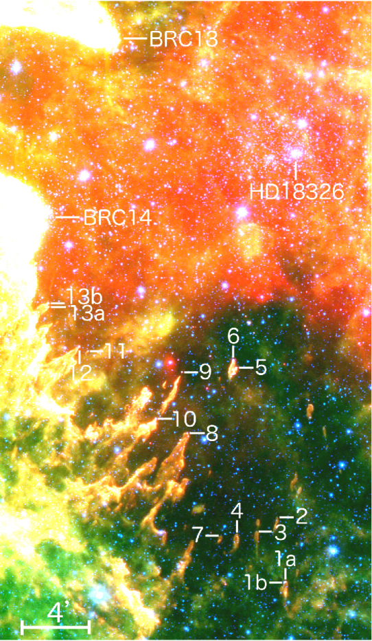
Figure 1: Contrast-enhanced Spitzer pseudo-color image of part of IC 1848E taken from the NASA Spitzer Space Telescope website. Stars at the tip of elephant trunk-like structures are marked together with two bright-rimmed clouds and the exciting star of IC 1848E. The scale is shown. North is up, east to the left.

2 Target Selection, Observations and Data Reduction

BRCs are small clouds apparently with both width and length of several arcminutes, corresponding to the physical size of a few parsecs typically (see Sugitani et al. 1991, Sugitani & Ogura 1994). In these papers BRCs are morphologically classified into types A, B and C according to their length-to-width ratios with type C being the most elongated. But many of the ETLSs found in figure 1 are much more elongated and of far smaller widths (typically one tenth of pc) than most of the type C BRCs in Sugitani et al. (1991) and Sugitani and Ogura (1994). We searched for such peculiar ETLSs that have a star/stars at their tip on the Spitzer 3.6 $\mu$m, 4.5 $\mu$m, and 8.0 $\mu$m images. Table 1 gives the results, listing such stars with running numbers identified in figure 1, the coordinates and some remarks. We refer to these stars as ETLS stars. Some of them are listed in Koenig et al. (2008, their Table 4).

Table 1: Stars at the tip of elephant trunk-like structures.

Star ID	$\alpha_{(2000)}$	$\delta_{(2000)}$	Identification & remarks
	(h:m:s)	($\circ$ : ′ : ′′)
1a	02:59:18.08	+60:08:37.7
1b	02:59:18.61	+60:08:34.5	brighter than 1a
2	02:59:23.28	+60:12:22.9
3	02:59:32.93	+60:11:32.1
4	02:59:42.33	+60:11:18.4
5	02:59:46.25	+60:21:09.7	K14
6	02:59:47.75	+60:21:36.6
7	02:59:49.66	+60:11:13.1
8	03:00:08.01	+60:17:12.1
9	03:00:12.21	+60:20:45.4
10	03:00:23.54	+60:17:55.1	K15
11	03:00:57.52	+60:21:44.0
12	03:01:01.97	+60:21:57.7	K16
13a	03:01:17.42	+60:24:13.4
13b	03:01:17.55	+60:24:25.0	K17?

Note – K numbers are identifications from Table 4 of Koenig et al. (2008). The coordinates of K17 are between those of 13a and 13b. There is another star $5^{\prime\prime}.4$ NE of 13b. It is relatively bright in the optical, but presumably a field star unrelated to the ETLS in view of its positions on the $V/(V-I_{c})$ color-magnitude diagram and ${(J-H)/(H-K)}$ color-color diagram.

For the ETLS stars that are visible in the DSS 2 red image, we carried out photometric observations in the $V$ and $I_{c}$ bands using Himalaya Faint Object Spectrograph Camera (HFOSC) in the imaging mode mounted on the 2.0-m Himalayan Chandra Telescope (HCT) of the Indian Astronomical Observatory (IAO), Hanle, India on 2009 November 22, 23, and 24. HFOSC is equipped with a 2048 $\times$ 2048 pixel² CCD camera. The details of the site, HCT and HFOSC can be found at the HCT website (http://www.crest.ernet.in). The sky at the time of observations was photometric with a seeing size (FWHM) of $\sim$$1^{\prime\prime}.5$. A number of bias and twilight flat frames were also taken during the observing runs. The log of the HCT observations is tabulated in table 2.

Table 2: Log of observations.

$\alpha_{(2000)}$	$\delta_{(2000)}$	Filter & exposure (sec) $\times$ no. of frames	Date of observations
(h:m:s)	($\circ$ : ′ : ′′)		(yr-mm-dd)
02:59:18.6	+60:08:34	V:600$\times$3; I:200$\times$3	2009-11-22
03:20:07.0	+60:18:47	V:600$\times$3; I:200$\times$3	2009-11-23
03:00:44.7	+60:20:45	V:600$\times$2; I:200$\times$3	2009-11-24

Table 3: Photometric data for the ETLS stars.

Star	$V\pm\Delta V$	$I_{c}\pm\Delta I_{c}$	$J\pm\Delta J$	$H\pm\Delta H$	$K_{s}\pm\Delta K_{s}$	$[3.6]\pm\Delta[3.6]$	$[4.5]\pm\Delta[4.5]$	$[5.8]\pm\Delta[5.8]$	$[8.0]\pm\Delta[8.0]$	$[24]\pm\Delta[24]$	class†
ID	$(mag)$	$(mag)$	$(mag)$	$(mag)$	$(mag)$	$(mag)$	$(mag)$	$(mag)$	$(mag)$	$(mag)$
1b	$20.73\pm 0.08$	$17.59\pm 0.02$	$14.63\pm 0.04$	$12.72\pm 0.03$	$11.78\pm 0.03$	$11.04\pm 0.01$	$10.92\pm 0.01$	$10.74\pm 0.02$	$10.56\pm 0.06$	-	III
5∗	$19.49\pm 0.02$	$17.25\pm 0.01$	$16.14\pm 0.11$	$15.22\pm 0.11$	$14.38\pm 0.1$	$12.65\pm 0.01$	$11.9\pm 0.01$	$11.04\pm 0.01$	$9.9\pm 0.03$	$6.68\pm 0.16$	I
6	$20.13\pm 0.02$	$17.35\pm 0.01$	$15.41\pm 0.08$	$14.07\pm 0.06$	$12.96\pm 0.04$	$11.93\pm 0.01$	$11.27\pm 0.01$	$10.59\pm 0.01$	$9.63\pm 0.01$	$6.11\pm 0.12$	II
9∗	$19.81\pm 0.02$	$16.93\pm 0.01$	$15.08\pm 0.05$	$14.08\pm 0.05$	$13.5\pm 0.04$	$12.85\pm 0.01$	$12.41\pm 0.01$	$11.9\pm 0.02$	$10.99\pm 0.02$	$8.08\pm 0.06$	II
10∗	$17.4\pm 0.01$	$15.05\pm 0.01$	$13.38\pm 0.03$	$12.48\pm 0.03$	$11.96\pm 0.03$	$11.29\pm 0.01$	$10.91\pm 0.01$	$10.48\pm 0.01$	$9.9\pm 0.01$	$7.16\pm 0.14$	II
12	$18.66\pm 0.01$	$16.03\pm 0.01$	$14.31\pm 0.03$	$13.24\pm 0.03$	$12.64\pm 0.03$	$11.59\pm 0.01$	$11.08\pm 0.01$	$10.56\pm 0.01$	$9.73\pm 0.01$	$7.08\pm 0.08$	II
13b	$22.08\pm 0.09$	$18.19\pm 0.01$	$16.09\pm 0.11$	$14.84\pm 0.08$	$14.14\pm 0.08$	$13.01\pm 0.01$	$12.61\pm 0.01$	$12.06\pm 0.02$	$11.12\pm 0.05$	-	II

^∗ $V$ and $I_{c}$ magnitudes are averages of those obtained on different nights.
^† Koenig et al. (2008).

The data analyses were carried out at ARIES, Nainital, India. The initial processing of the data frames was done using various tasks available under the IRAF data reduction software package. Photometric measurements of the ETLS stars were performed by using DAOPHOT II software package (Stetson 1987). A point spread function (PSF) was obtained for each frame using several uncontaminated stars. The results of the measurements were transformed to the standard system by using the secondary standards taken from Chauhan et al. (2011). The photometric accuracies depend on the brightness of the stars, and the typical DAOPHOT errors in the $V$ and $I_{c}$ bands at $V$ $\sim$ 18 are smaller than 0.01 mag. Near the limiting magnitude of $V$ $\sim$ 22 they increase to 0.1 and 0.02 mag in the $V$ and $I_{c}$ bands, respectively.

Since young stellar objects (YSOs) often show NIR/MIR excesses caused by circumstellar disks, NIR/MIR photometric data are very important to know their nature and evolutionary status. $JHK_{s}$ data for the ETLS stars have been obtained from the 2MASS Point Source Catalog (PSC) (Cutri et al. 2003). Also we tried to collect Infrared Array Camera (IRAC) 3.6 $\mu$m, 4.5 $\mu$m, 5.6 $\mu$m, and 5.8 $\mu$m data and Multiband Imaging Photometer for Spitzer (MIPS) 24 $\mu$m photometry for them from Koenig et al. (2008)’s list of stars in the W5 region. We searched for the 2MASS and Spitzer MIR counterparts of the ETLS stars and identified them using a search radius of $1.^{\prime\prime}2$. The photometric data for the stars are given in table 3.

3 Results

3.1 NIR Color-color Diagram

Figure 2a (left) shows the ${(J-H)/(H-K)}$ NIR color-color diagram (CCD) for the ETLS stars identified in the 2MASS PSC catalogue. The solid and long-dashed curves represent the unreddened main sequence and giant branches (Bessell $\&$ Brett 1988), respectively. The dotted line indicates the loci of intrinsic classical T Tauri stars (CTTSs) (Meyer et al. 1997). The parallel dashed lines are reddening vectors drawn from the tip (spectral type M4) of the giant branch (“upper reddening line”), from the base (spectral type A0) of the main sequence branch (“middle reddening line”) and from the tip of the intrinsic CTTS line (“lower reddening line”). The extinction ratios $A_{J}/A_{V}=0.265,A_{H}/A_{V}=0.155$, and $A_{K}/A_{V}=0.090$ have been adopted from Cohen et al. (1981). All of the star positions and lines are in the CIT system. We classify the NIR CCD into three zones (‘F’, ‘T’, and ‘P’) to study the nature of the sources (for details see Ojha et al. 2004a, b). The ‘F’ sources are located between the upper and middle reddening lines and are considered to be either main-sequence stars or weak-line T Tauri stars or CTTSs with small NIR excesses. ‘T’ sources are located between the middle and lower reddening lines and are considered to be mostly CTTSs/Class II objects with large NIR excesses. The sources in the ‘P’ region are most likely Class I stars (protostar-like objects), surrounded by an envelope. In figure 2a ETLS stars having a 2MASS counterpart, are plotted with different symbols according to the classifications by Koenig et al. (2008) based on the Spitzer data. Sources of class I, class II, and class III are shown by filled circles, by triangles, and by open circles, respectively. We estimated $A_{V}$ for each star by tracing them back to the intrinsic CTTS line of Meyer et al. (1997) along the reddening vector (for details, see Ogura et al. 2007). The mean of the individual $A_{V}$ values turned out to be $A_{V}$ = $2.4\pm 1.2$ mag or $E(V-I_{c})$ = $0.96\pm 0.48$ mag, which we use in further discussions.

3.2 Optical Color-Magnitude Diagram

Figure 2: (a, left) ${(J-H)/(H-K)}$ CCD for the ETLS stars. Their classifications are taken from Koenig et al. (2008), which are based on the $Spitzer$ data. The solid and thick dashed curves represent the unreddened main sequence and giant branches (Bessell & Brett 1988), respectively. The dotted line indicates the loci of intrinsic CTTSs (Meyer et al. 1997). The parallel dashed lines are the reddening vectors drawn from the tip of the giant branch, from the base of the main sequence branch and from the tip of the intrinsic CTTS line with crosses representing a visual extinction of $A_{V}$ = 5 mag. (b, right) $V/(V-I_{c})$ CMD for the ETLS stars. The PMS isochrones and evolutionary tracks from Siess et al. (2000) are overplotted. The thick continuous line is the zero-age main sequence (ZAMS) from Girardi et al. (2002). The isochrones and evolutionary tracks are corrected for the distance 2.1 kpc and the mean reddening $E(V-I_{c})=0.96$ mag (see the text). The dashed arrow shows the reddening vector corresponding to $A_{V}$ = 2 mag.

In figure 2b (right) we give the $V/(V-I_{c})$ CMD of the ETLS stars listed in Table 3. The PMS isochrones and evolutionary tracks of Siess et al. (2000) as well as the zero-age main sequence of Girardi et al. (2008) are overlaid after being shifted to the distance modulus 13.5 mag (distance of 2.1 kpc; Chauhan et al. 2011) and the mean reddening of $E(V-I_{c})$ = 0.96 mag. Note that the positions of the stars are not corrected for their reddening values. But the effect of the variable reddenings on the age estimation is small, because the reddening vector is nearly parallel to the $V/(V-I_{c})$ PMS isochrones, as indicated in figure 2b. This CMD manifests that these sources are actually PMS stars having ages of 0.2 - 5 Myr and masses of 0.1 - 1 $M_{\odot}$. We presume that these stars are physically related to the ETLSs because of their location at their very tip. However the possibility that some of them are field stars (foreground main- sequence or background giant stars) can not be entirely rejected, since the southern part of IC 1848E is located at a very low $galactic$ latitude (l $\sim$ 1.5^∘).

3.3 Spectral Energy Distribution Fitting

To understand the nature and evolutionary status of the ETLS stars we re-construct their SEDs using the recently available grid of models and fitting tools of Robitaille et al. (2006, 2007). The models were computed using a Monte Carlo based radiation transfer codes (Whitney et al. 2003a, 2003b) assuming several combinations of a PMS central star, a flared accretion disk, a rotationally flattened infalling envelope and a bipolar cavity for a reasonably large parameter space. Interpreting SEDs using radiative transfer codes is subject to degeneracies, which spatially-resolved multiwavelength observations can overcome. The SED fitting tools fit these models to observational data points while assuming the distance and foreground reddening as being free parameters. For IC 1848 the distance in the literature varies from 1.9 to 2.3 kpc (Hillwig et al. 2006, Moffat 1972, Becker & Fenkart 1971). Hence, we have taken the distance to be in the range of 1.9 to 2.3 kpc. Based on the NIR CCD (figure 2a), we assumed the visual absorption ($A_{V}$) ranges from 2 to 10 mag for these sources. We set the uncertainties of the NIR and MIR flux estimates to be 10 to 15%. We calculate a goodness-of-fit parameter, $\chi^{2}$, normalized by the number of data points $N_{data}$ (9 or 10) used in the fitting. The evolutionary parameters of each source are determined by using the average of all the “well-fitted” models. The well-fitted models of each source are defined by

$\chi^{2}$ - ${\chi^{2}}_{min}$ $\leq$ $2N_{data}$

where ${\chi^{2}}_{min}$ is the goodness-of-fit parameter of the best fit model. In table 4 we tabulate for each source the average parameters, such as the age, the interstellar extinction ($A_{V}$, which does not include the extinction due to the circumstellar disk or envelope), the mass of the star ($M_{star}$), the disk accretion rate ($\dot{M}_{disk}$), and the envelope accretion rate ($\dot{M}_{env}$). Here, it is worth mentioning that these are crude values, and should be considered to only be approximate in view of the underlying assumptions in the models. Also, the number of observational data points is limited in spite of many parameters involved. The stellar ages given in table 4 range from 0.2 to 5 Myr again, although the results for individual stars differ from those derived from the $V/(V-I_{c})$ CMD. Figure 3 shows three examples of the SED fitting.

Table 4: Physical parameters for the ETLS stars based on the SED fitting.

Star	Age	$A_{V}$	$M_{star}$	$M_{disk}$	$\dot{M}_{disk}$	$\dot{M}_{env}$	${\chi^{2}}_{min}$	$N_{data}$
ID	(Myr)	(mag)	($M_{\odot}$)	($M_{\odot}$)	(10-8$M_{\odot}$/yr)	(10-6$M_{\odot}$/yr)
1b	$0.2\pm 0.1$	$3.8\pm 0.8$	$1.8\pm 1.2$	$0.01\pm 0.03$	$11.0\pm 11.0$	$14.0\pm 18.0$	5.36	9
5	$4.4\pm 3.1$	$3.1\pm 0.6$	$2.4\pm 0.3$	$0.02\pm 0.02$	$0.12\pm 0.12$	$1.3\pm 1.7$	25.85	10
6	$5.5\pm 3.6$	$5.5\pm 1.5$	$2.0\pm 1.3$	$0.01\pm 0.02$	$14.0\pm 1.8$	$1.1\pm 11.0$	9.20	10
9	$2.8\pm 2.1$	$4.3\pm 0.8$	$1.6\pm 0.5$	$0.01\pm 0.01$	$0.5\pm 0.5$	$0.03\pm 0.14$	5.06	10
10	$1.0\pm 0.9$	$3.2\pm 0.6$	$2.2\pm 0.8$	$0.01\pm 0.01$	$1.4\pm 1.3$	$0.57\pm 1.2$	2.15	10
12	$4.8\pm 2.6$	$5.1\pm 0.8$	$2.3\pm 0.6$	$0.01\pm 0.01$	$3.9\pm 3.6$	$0.1\pm 0.4$	5.31	10
13b	$2.3\pm 2.3$	$5.4\pm 1.0$	$2.1\pm 0.9$	$0.01\pm 0.01$	$1.6\pm 1.5$	$6.8\pm 16.9$	7.44	9

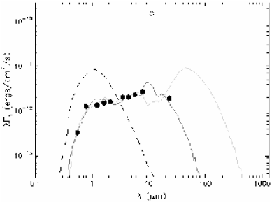
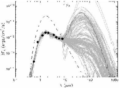
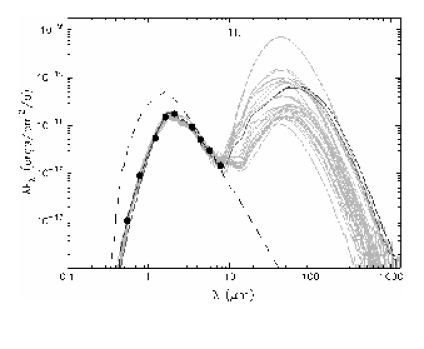
Figure 3: SEDs for a Class I, Class II and Class III sources among the ETLS stars. The black lines represent the best fits, and the gray lines subsequent good fits. The dashed lines show the stellar photospheres corresponding to the central sources of the best-fit models. The filled circles are the input flux values.

4 Discussion

4.1 Origin of Bright-Rimmed Clouds and Hydrodynamical Instability of Ionization Fronts

The effects of intense UV radiation from OB stars on star formation can be either constructive or destructive, depending on the situation. As for the mechanisms with which it works constructively, two have so far been proposed: collect-and-collapse and radiation-driven implosion (RDI). The former/latter is of larger/smaller size in space ($\sim$10 pc/$\sim$1 pc) and of longer/shorter timescale ($\sim$a few Myr/$\sim$0.5 Myr).

Collect-and-collapse was advocated by Elmegreen and Lada (1977) in their hypothesis of Sequential Star Formation. In this scenario, pressure-driven expansion of an HII region collects a dense shell between the ionization front (IF) and shock front (SF), which in due time becomes gravitationally unstable and collapses to form stars of the second generation including OB stars. Since then various analytic and numerical calculations were carried out under this scenario. However, it has never been convincingly confirmed for many years, until very recently when the Deharveng group (Deharveng et al. 2005; Pomarès et al. 2009, and references therein) presented the first persuasive examples. This mechanism is probably viable in relatively uniform molecular clouds.

RDI takes place in small molecular clouds, which are called “bright-rimmed clouds (BRCs)”, “globules”, “elephant trunks” and so forth. They are usually considered to be remnant cloud clumps left over in expanding HII regions. Detailed numerical calculations (e.g., Lefloch & Lazareff 1994) showed that such clouds are compressed by the high pressure of the surrounding HII gas. Star formation in BRCs was suspected from early times (e.g., Wootten et al. 1983). Clear evidence for star formation in these clouds was provided by Sugitani, Fukui, and Ogura (1991) and Sugitani and Ogura (1994), who showed their association with IRAS point sources of low temperatures. Also, Sugitani, Tamura, and Ogura (1995) indicated that BRCs are often associated with a small star cluster, showing not only an asymmetric spatial distribution, but also a possible age gradient. This lead them to advocate the hypothesis of “small-scale sequential star formation”, which has recently been verified quantitatively by BVI_c photometry by Ogura et al. (2007) and Chauhan et al. (2009, 2011). Detailed observations of physical properties of BRCs cataloged in Sugitani et al. (1991) and Sugitani and Ogura (1994) were made by the British group (Morgan et al. 2008, Urquhart, Morgan & Thompson 2009, and references therein) by means of sub-millimeter observations and radio continuum and CO/¹³CO/C¹⁸O line observations. They concluded that RDI is in progress in many (but not all) of these BRCs, and that relatively massive stars are being formed there, based on the high luminosity of the embedded sources (Urquhart et al. 2009).

As for the origin of BRCs or elephant trunks, a Rayleigh-Taylor instability in expanding HII regions was proposed first (e.g., Spitzer 1954), but Pottasch (1958) pointed out disagreements between their morphology and the theoretical predictions. In mid-1960s Axford (1964) investigated the stability of weak D-type IFs, explicitly taking into account the effect of diffuse UV radiation caused by recombinations to the ground state of hydrogen atoms. He claimed that weak D-type IFs, which correspond to the major part of the evolution of HII regions, are stable against the growth of wavelengths larger than 0.2 pc, so hydrodynamical instability could not be the origin of elephant trunks. Given the fact that radio observations showed the clumpiness of molecular clouds, BRCs or elephant trunks have since then been usually considered to be pre-existing cloud clumps left over in expanding HII regions. Sysoev (1997) re-examined the stability of D-type IFs analytically and showed that, contrary to the conclusion by Axford (1964), they are not stable even with the effect of the recombinations. This new result was confirmed by numerical simulations of Williams (2002). Prior to these studies, Giuliani (1979) investigated the stability of the combined systems of a D-type IF and a preceding SF and reached a similar conclusion that there is a new regime of instability (longer wavelengths which are similar to the widths of the above structures) that grows rapidly in an oscillatory manner (overstability). Vishniac (1983) generalized this instability including SN/wind bubble SFs, and it is now called as “thin shell instability” or “Vishniac instability”. Its mechanism is simple, as shown, e.g., in figure 1 of García-Segura and Franco (1996). The presence of an IF exacerbates the growth of the instability.

Thus, BRC- or globule-like structures seem to be also formed via hydrodynamical instability without pre-existing molecular clumps. This was clearly shown in numerical simulations (2-dimensional) of the evolution of HII regions by García-Segura and Franco (1996); such structures arise in all of their models as HII regions expand. In their 3-D simulations Whalen and Norman (2008) obtained very similar results to those of García-Segura and Franco (1996). Other recent numerical simulations of evolution of HII regions with turbulence (Mellema et al. 2006; Dale, Clark & Bonell 2007; Gritschneder et al. 2009, 2010) and without turbulence (Mizuta et al. 2006; Bisbas et al. 2009) all show the formation of BRC- or globule-like structures. But, since molecular clouds are very clumpy, it seems more likely that ordinary BRCs have their origin in pre-existing clumps.

Figure 4: Distribution of the widths of the head part of 41 ETLSs found in figure 1 as well as that of 6 BRCs listed in Ogura et al. (2002) in the whole IC 1848. Note that the abscissa scale of the right-hand half of the figure is two times smaller than that of the left-hand half.

As for ETLSs, we suppose that their origin is different from that of ordinary BRCs and that they presumably originate from the above-mentioned hydrodynamical instability, based on the following three reasons. First, as mentioned already, the morphologies are very different; ETLSs are much thinner and more elongated than BRCs. Second, ETLSs and BRCs have different size distributions. Figure 4 shows the distribution of the widths of the head part of 41 ETLSs found in figure 1. That of BRCs is also shown for comparison; there are 6 BRCs listed in Ogura et al. (2002) in the whole IC 1848, i.e., BRCs 11, 11NE, 11E, and 12 in IC 1848W, and BRCs 13 and 14 in IC 1848E. Note that the abscissa scale of the right-hand half of the figure is two times smaller than that of the left-hand half. Also, the number for the smallest bin may be affected by the incompleteness in picking up tiny ETLSs. The histogram shows a clear gap between the distributions of ETLSs and BRCs. Also, the combined size distribution of ETLSs and BRCs as well as that of the former, itself, does not exhibit any power laws, contrary to the well-known power-law core mass function (above a certain mass) (see, e.g., Sadavoy et al. 2010). There seems to be a peak at around 0.1 pc. It might reflect the characteristic wavelength of the hydrodynamical instability in the IC 1848E HII region. The third reason is the fact that generally the ETLS stars are slightly younger than the stars associated with BRCs in IC 1848E. Figure 2b indicates the ETLS stars have ages of 0.2 - 1.0 Myr except for star No. 5. On the other hand, Chauhan et al. (2009) obtained 0.5 - 5 Myr and 0.1 - 3 Myr for majorities of the stars associated with BRCs 13 and 14, respectively (see their Figure 2). Chauhan et al. (2011) revisited these BRCs, and the results are 0.5 - 5 Myr and 0.3 - 5 Myr, respectively (see their figure 9). From the very elongated morphology of the ETLSs one can imagine that they might be an older version of BRCs of the similar type, i.e., type C that formed from pre-existing clumps. But the above ages defy this conjecture.

4.2 Third Possible Mechanism of Triggered Star Formation

On the basis of the result that the ETLS stars in IC 1848E are of the PMS nature having ages of 0.2 - 5 Myr and masses of 0.1 - 1 $M_{\odot}$ , we consider that they formed under the compressing effects of the HII gas from these small clouds, which were created by a hydrodynamical instability of the expanding HII region. Thus, this process seems to make a third mode of triggered star formation associated with HII regions, in addition to collect-and-collapse and RDI.

This new mechanism of triggered star formation is somewhat similar to the RDI in BRCs, but it differs in that the cloud was not pre-existing but formed from accumulated and then fragmented gas in the process of expansion of an HII region. In addition, we find only one star or at most a few stars at the tip of each ETLS, so the scale of star formation in each cloud is very small. However, the total product can be considerable because a large number of such structures can be formed in an HII region, as in IC 1848E. In our recent studies on BRC star formation we noticed many IR-excess stars scattered inside HII regions besides IC 1848E (see Fig. A3 of Chauhan et al. 2009). We suspect that some of these stars may have been formed by this mechanism. On the Spitzer IRAC images of the Carina Nebula Smith et al. (2010) also found a large number of scattered YSOs as well as many clouds morphologically similar to our ETLSs. Table 5 summarizes the differences of this mechanism from collect-and-collapse and usual RDI.

Table 5: Comparison of modes of triggered star formation.

mode	cloud	scale	stars formed	timescale
collect & collapse	accumulated	large	$>$ 300	a few Myr
RDI	pre-existing	small	$<$ 100	$<$ 1 Myr
HD instability	accumulated	small	$\leq$ a few	$<$ 1 Myr

5 Conclusions

We paid attention to the numerous, elephant trunk-like clouds in IC 1848E and carried out $VI_{c}$ photometry of the optically visible stars located at the tip of several of them. Their positions on the $V/V-I_{c}$ CMD indicate that they are low-mass PMS stars of ages of mostly one Myr or less. The physical parameters derived for these stars by using the SED fitting tools indicate that they are largely Class I or Class II PMS sources. The PMS nature of these stars strongly suggests that they must have formed from these ETLSs. On the basis of the morphology, the size distributions, and the ages of the associated young stars we conclude that the ETLSs and BRCs have different origins, and suspect that the former are created by the hydrodynamical instability of the IF/SF of the expanding HII region. We further hypothesize that, in addition to the collect-and-collapse process and RDI, this mechanism makes a third mode of triggered star formation associated with HII regions.

6 Acknowledgement

We are grateful to the anonymous referee for his/her useful comments that improved this paper. We thank the staff of IOA, Hanle and CREST, Hosakote for the assistance during the observations. NC is thankful to the fellowship granted by DST and CSIR, India. KO and AKP acknowledge JSPS, Japan and DST, India for the financial supports.

References

- [1] Axford W. I. 1964, ApJ, 140, 112
- [2] Becker W., & Fenkart R. 1971, A&AS, 4, 241
- [3] Bessell M. S., & Brett J. M. 1988, PASP, 100, 1134
- [4] Bisbas T. G., Wuensch R., Whitworth A. P., & Hubber D. A. 2009, A&A, 497, 649
- [5] Chauhan N., Pandey A. K., Ogura K., Ojha D. K., Bhatt B. C., Ghosh S. K., & Rawat P. S. 2009, MNRAS, 396, 964
- [6] Chauhan N., Pandey A. K., Ogura K., Jose J., Ojha D. K., Samal M. R., & Mito H. 2011, MNRAS, in press
- [7] Cohen J. G., Frogel J. A., Persson S. E., & Elias J. H. 1981, ApJ, 249, 481
- [8] Cutri R. M., et al. 2003, The IRSA 2MASS All Sky Point Source Catalog, NASA/IPAC Infrared Science Archive, http://irsa.ipac.caltech.edu/applications/Gator/
- [9] Dale J. E., Clark P. C., & Bonnell I. A. 2007, MNRAS, 377, 535
- [10] Deharveng L., Zavagno A., & Caplan J. 2005, A&A, 433, 565
- [11] Elmegreen B. G., & Lada C. J. 1977, ApJ, 214, 725
- [12] García-Segura G., & Franco J. 1996, ApJ, 469, 171
- [13] Girardi L., Bertelli G., Bressan A., Chiosi C., Groenewegen M. A. T., Marigo P., Salasnich B., & Weiss A. 2002, A&A, 391, 195
- [14] Giuliani J. L. Jr. 1979, ApJ, 233, 280
- [15] Gritschneder M., Naab T., Walch S., Burkert A., & Heitsch F. 2009, ApJ, 694, L26
- [16] Gritschneder M., Burkert A., Naab T., & Walch S. 2010, ApJ, 723, 971
- [17] Hillwig T. C., Gies D. R., Bagnuolo W. G., Jr., Huang W., McSwain M. V., & Wingert D. W. 2006, ApJ, 639, 1069
- [18] Koenig X. P., Allen L. E., Gutermuth R. A., Hora J. L., Brunt C. M., & Muzerolle J. 2008, ApJ, 688, 1142
- [19] Lefloch B., & Lazareff B. 1994, A&A, 289, 559
- [20] Mellema G., Arthur S. J., Henney W. J., Iliev I. T., & Shapiro P. R. 2006, ApJ, 647, 397
- [21] Meyer M. R., Calvet N., & Hillenbrand L. A. 1997, AJ, 114, 288
- [22] Mizuta A., Kane J. O., Pound M. W., Remington B. A., Ryutov D. D., & Takabe H. 2006, ApJ, 647, 1151
- [23] Moffat A. F. J. 1972, A&AS, 7, 355
- [24] Morgan L. K., Thompson M. A., Urquhart J. S., & White G. J. 2008, A&A, 477, 557
- [25] Ogura K., Chauhan N., Pandey A. K., Bhatt B. C., Ojha D., & Itoh Y. 2007, PASJ, 59, 199
- [26] Ojha D. K., et al. 2004a, ApJ, 608, 797
- [27] Ojha D. K., et al. 2004b, ApJ, 616, 1042
- [28] Pomarès M., et al. 2009, A&A, 494, 987
- [29] Pottasch S. 1958, Bull. Astron. Inst. Netherlands, 14, 29
- [30] Robitaille T. P., Whitney B. A., Indebetouw R., & Wood K. 2007, ApJS, 169, 328
- [31] Robitaille T. P., Whitney B. A., Indebetouw R., Wood K., & Denzmore P. 2006, ApJS, 167, 256
- [32] Sadavoy S. I., et al. 2010, ApJ, 710, 1247
- [33] Siess L., Dufour E., & Forestini M. 2000, A&A, 358, 593
- [34] Smith N., et al. 2010, MNRAS, 406, 952
- [35] Spitzer L. Jr. 1954, ApJ, 120, 1
- [36] Stetson P. B. 1987, PASP, 99, 191
- [37] Sugitani K., Fukui Y., & Ogura K. 1991, ApJS, 77, 59
- [38] Sugitani K., & Ogura K. 1994, ApJS, 92, 163
- [39] Sugitani K., Tamura M., & Ogura K. 1995, ApJ, 455, L39
- [40] Sysoev N. E. 1997, Astron. Lett., 23, 409
- [41] Urquhart J. S., Morgan L. K., & Thompson M. A. 2009, A&A, 497, 789
- [42] Vishniac E. T. 1983, ApJ, 274, 152
- [43] Whalen D. J., & Norman M. L. 2008, ApJ, 672, 287
- [44] Whitney B. A., Wood K., Bjorkman J. E., & Cohen M. 2003b, ApJ, 598, 1079
- [45] Whitney B. A., Wood K., Bjorkman J. E., & Wolff M. J. 2003a, ApJ, 591, 1049
- [46] Williams R. J. R. 2002, MNRAS, 331, 693
- [47] Wootten A., Sargent A., Knapp G., & Huggins P. J. 1983, ApJ, 269, 147
- [48] Zavagno A., Pomarès M., Deharveng L., Hosokawa T., Russeil D., & Caplan J. 2007, A&A, 472, 835