Buckled nano rod - a two state system: quantum effects on its dynamics

Abstract

We consider a suspended elastic rod under longitudinal compression. The compression can be used to adjust potential energy for transverse displacements from harmonic to double well regime. The two minima in potential energy curve describe two possible buckled states. Using transition state theory (TST) we have calculated the rate of conversion from one state to other. If the strain $\varepsilon=4\varepsilon_{c}$ the simple TST rate diverges. We suggest a method to correct this divergence for quantum calculations. We also find that zero point energy contributions can be quite large so that single mode calculations can lead to large errors in the rate.

I Introduction

Considerable attention has recently been paid to two-state nano-mechanical systems Roukes ; Craighead ; Park ; Erbe ; ClelandAPL ; Rueckes ; Blencowe and the possibility of observing quantum effects in them. Roukes et al. Roukes proposed to use an electrostatically flexed cantilever to explore the possibility of macroscopic quantum tunnelling in a nano-mechanical system. Carr et al. Carr ; ClelandAPL suggested using the two buckled states of a nanorod and investigated the possibility of observing quantum effects. A suspended elastic rod of rectangular cross section under longitudinal compression is considered. As the compressional strain is increased to the buckling instability Carr , the frequency of the fundamental vibrational mode drops continuously to zero. Beyond the instability, the system has a double well potential for the transverse motion (see Fig. 1). The two minima in the potential energy curve describe the two possible buckled states at that particular strain Carr and the system can change from one to the other by thermal fluctuations or quantum tunneling. Since both the well depth and assymetry are tunable, a variety of quantum phenomena can be explored, including zero-point fluctuations, tunneling and coherent superposition of macroscopically distinct states. In this paper we have calculated the rate of transition between the two thermally equilibrium states of a buckled nanorod/nanotube at fixed strain using quantum mechanical version of transition state theory. Although this mechanical system has analogies to the superconducting interference device in which the first observation of a coherent superposition of macroscopically distinct states was reported Friedman , but our method strictly address the thermally induced incoherent relaxation rate from one buckled state to the other at a fixed strain. It may be possible by compressing a silicon nanorod or a carbon nanotube at low temperature to cause a crossover between the quantum and thermal fluctuation regime. In an earlier paper we have analyzed the classical version of this problem Sayan .

II The model

We use $L$, $w$ and $d$ (satisfying $L>>w>>d$) to denote the length, width and thickness of the rod Carr ; Wybourne ; CarrAPL ; Lawrence . $F$ is the linear modulus (energy per unit length) of the rod and is related to the elastic modulus $Q$ of the material by $F=Qwd$. The bending moment $\kappa$ is given by $\kappa^{2}=d^{2}/{12}$ Carr ; Morse for a bar of rectangular cross section. We take the length of the uncompressed rod to be $L_{0}$. We apply compression on the two ends, reducing the separation between the two to $L$. If $y(x)$ denotes the displacement of the rod in the ‘$d$’ direction,

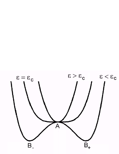
Figure 1: Potential energy $V$ as a function of the fundamental mode displacement $Y$. The shape of the potential energy is harmonic for $\varepsilon>\varepsilon_{c}$, quartic for $\varepsilon=\varepsilon_{c}\equiv$ critical strain ($\varepsilon_{c}<0$) and a double well for $\varepsilon<\varepsilon_{c}$.

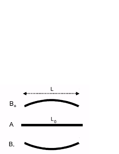
Figure 2: The rod under compression: The central figure (A) shows the uncompressed rod of length $L_{0}$. On compressing to length $L$, the rod buckle, either to $B_{-}$ or to $B_{+}$.

then the length of the rod $L_{total}=\int_{0}^{L}dx\sqrt{1+(y^{\prime})^{2}}\approx L+1/2\int_{0}^{L}dx(y^{\prime})^{2}$. The compression causes a contribution to the potential energy

$$V_{elastic}=F/(2L_{0})(L_{total}-L_{0})^{2}.$$ (1)

In addition, bending of the rod in the ‘$d$’ direction cause bending energy

$$V_{b}=F\kappa^{2}/{2}\int_{0}^{L}dx(y^{\prime\prime})^{2}.$$ (2)

Thus the total potential energy is given by

$$V[y(x)]={1}/{2}\int_{0}^{L}dx(F\kappa^{2}(y^{\prime\prime})^{2}+F\varepsilon(y^{\prime})^{2})+{F}/(8L_{0})(\int_{0}^{L}dx(y^{\prime})^{2})^{2}+{F}/(2L_{0})(L-L_{0})^{2}.$$ (3)

Here $\varepsilon=(L-L_{0})/L_{0}$ is the strain.

III Extrema of the functional V[y(x)]

Extremisation of potential energy functional with respect to $y(x)$ leads to

$$F\kappa^{2}\frac{\partial^{4}y}{\partial x^{4}}-[F\varepsilon\frac{\partial^{2}y}{\partial x^{2}}+\frac{F}{2L_{0}}(\int_{0}^{L}dx(y^{\prime}(x))^{2})\frac{\partial^{2}y}{\partial x^{2}}]=0$$ (4)

and the hinged end points have boundary conditions $y(0)=y(L)=0$ and $y^{\prime\prime}(0)=y^{\prime\prime}(L)=0$ (hinged boundary conditions are chosen for computational simplicity). If $\varepsilon>\varepsilon_{c}=-\kappa^{2}\pi^{2}/{L^{2}}$ then, the only solution to Eq. (4) is $y(x)=0$ if $\varepsilon>\varepsilon_{c}$. But if $\varepsilon<\varepsilon_{c}$, two bucked states are possible. They are

$$y(x)=\pm A\sqrt{{2}/{L}}\sin({\pi}x/{L}),$$ (5)

with $A=\sqrt{{2L_{0}L^{2}}(\varepsilon_{c}-\varepsilon)/{\pi^{2}}}$. For $\varepsilon<\varepsilon_{c}$, all the normal modes of vibration about these are stable. The solution $y(x)=0$ is now a saddle point.

IV The Dynamics

One can calculate the barrier height for the process of going from one buckled state to the other over the saddle (linear geometry) as

$$\Delta E_{Barrier}^{Linear}={FL_{0}}(\varepsilon-\varepsilon_{c})^{2}/{2}.$$ (6)

The kinetic energy of the rod is $\mu/2\int_{0}^{L}y_{t}^{2}dx$, where $\mu={m}/{L_{0}}$ is the mass per unit length. Using the boundary conditions for the hinged end points, we find the normal modes of the rod, $y(x,t)=y_{n}(x)e^{i\omega_{n}t}$. At the saddle point, we obtain

$$y_{n}(x)=A_{n}\sqrt{{2}/{L}}\sin({n\pi x}/{L}),$$ (7)

with $n=1,2,3...$. The normal mode frequencies at the saddle point are given by

$$\omega_{Linear,n}^{\ddagger}=\omega_{0}\;n\,\sqrt{n^{2}-{\varepsilon}/{\varepsilon_{c}}},$$ (8)

where $\omega_{0}={\pi^{2}\kappa}/{L^{2}}\sqrt{{F}/{\mu}}$. $n=1$ is the unstable mode and it has the imaginary frequency

$$\omega_{Linear,1}^{\ddagger}=i\Omega_{Linear},$$ (9)

where $\Omega_{Linear}=\omega_{0}\;\,\sqrt{{\varepsilon}/{\varepsilon_{c}}-1}$. For the buckled state, the normal modes are the same as at the saddle point, but the normal mode frequencies are different. They are

$$\omega_{n}=\omega_{0}n\sqrt{n^{2}-1}\;\;\;{\text{f}orn>1},$$ (10)

while $\omega_{1}=\omega_{0}\sqrt{2\left({\varepsilon}/{\varepsilon_{c}}-1\right)}$. The rate expression using classical TST is (Eq. 3.14 of reference Hanggi ) is

$$R_{f}^{classical}=\Omega_{Linear}\prod_{n=1}^{N}\left|{\omega_{n}}/{\omega_{Linear,n}^{\ddagger}}\right|e^{-\Delta E_{Barrier}^{Linear}/kT},$$ (11)

where $N$ denotes the total number of transverse modes of the rod. One makes a negligible error by taking the value of $N$ to be infinity and this leads to Sayan

$$R_{f}^{classical}=\frac{\sqrt{F}}{2L\sqrt{\mu}}\sqrt{\Gamma\left(2-\sqrt{\frac{\varepsilon}{\varepsilon_{c}}}\right)\Gamma\left(2+\sqrt{\frac{\varepsilon}{\varepsilon_{c}}}\right)(\varepsilon_{c}-\varepsilon)}e^{-\frac{FL_{0}}{2kT}(\varepsilon-\varepsilon_{c})^{2}}.$$ (12)

The rate expression using quantum TST is given by

$$R_{f}^{quantum}=\frac{\Omega_{Linear}e^{-\frac{FL_{0}}{2kT}(\varepsilon-\varepsilon_{c})^{2}}}{2\pi\sin(\frac{\hbar\Omega_{Linear}}{2kT})}\sinh(\frac{\hbar\omega_{1}}{2kT})\prod\limits_{n=2}^{N}\frac{\sinh(\frac{\hbar\omega_{n}}{2kT})}{\sinh(\frac{\hbar\omega_{Linear,n}^{\ddagger}}{2kT})}.$$ (13)

The above rates have a problem. As $\sqrt{{\varepsilon}/{\varepsilon_{c}}}\rightarrow 2$, $\omega_{Linear,2}^{\ddagger}\rightarrow 0$ the second buckling instability sets in and the rates diverge. Also the quantum rate expression diverge at temperature $T={\hbar\Omega_{Linear}}/({2k\pi})$.

V Beyond The Second Buckling Instability

As the rod is compressed, first the mode $A_{1}\sqrt{{2}/{L}}\sin({\pi x}/{L})$ becomes unstable and this is the first buckling instability and the rod buckles as a result of this. The length at which this occurs shall be denoted by $L_{f}$. If one supposes that the rod is compressed further keeping the straight rod configuration, then at a length $L_{s}$, the mode $A_{2}\sqrt{{2}/{L}}\sin({2\pi x}/{L})$ too would become unstable and this is the second buckling instability.

Figure 3: Plot of $\Delta E_{Barrier}^{Linear}$ against ($L-L_{0}$) for a silicon rod of dimensions $L_{0}=1000\>\AA$, $w=200\>\AA$ and $d=100\>\AA$. For this rod the first two buckling instabilities occur at $L_{f}-L_{0}=-8.364\>\AA$ and $L_{s}-L_{0}=-35.354\>\AA$ respectively. The first buckling instability is shown by an arrow and the second buckling instability is not shown in figure.

Figure 4: Plot of barrier height against ($L-L_{0}$), for a silicon rod of dimensions $L_{0}=500\>\AA$,$w=20\>\AA$, $d=10\>\AA$. For this rod the first three buckling instabilities occur at $L_{f}-L_{0}=-0.1646\>\AA$, $L_{s}-L_{0}=-0.6597\>\AA$ and $L_{t}-L_{0}=-1.4893\>\AA$ respectively. The first two buckling instabilities are shown in figure using arrows and the third buckling instability is not shown in figure. Solid line is for linear saddle point (valid in the regime $L>L_{s}$ ), dashed line is for bent saddle point (valid in the regime $L<L_{s}$).

For $\varepsilon>4\varepsilon_{c}$, there is only one saddle point. But for $\varepsilon<4\varepsilon_{c}$, due to the second instability, the saddle point bifurcates into two. In a similar fashion one can have the third instability at a length $L_{t}$ etc. In order to analyze the rate near and beyond the second buckling instability, we assume that the displacement has the form

$$y_{0}(x)=A_{1}\sqrt{{2}/{L}}\sin({\pi x}/{L})+A_{2}\sqrt{{2}/{L}}\sin({2\pi x}/{L}).$$ (14)

Using this, the elastic potential energy is given by

$$V(A_{1},A_{2})=\frac{F\pi^{4}(A_{1}^{2}+4A_{2}^{2})^{2}}{8L^{4}L_{0}}+\frac{F\pi^{2}A_{1}^{2}(\varepsilon-\varepsilon_{c})}{2L^{2}}+\frac{2F\pi^{2}A_{2}^{2}(\varepsilon-4\varepsilon_{c})}{L^{2}}.$$ (15)

Figure 5: Plot of $\Delta E_{Barrier}^{Linear}$ against ($L-L_{0}$), for a multiwalled carbon nanotube of dimensions $L_{0}=5000\>\AA$, $d_{1}=50\>\AA$, $d_{2}=100\>\AA$. For this nanotube the first two instabilities occur at $L_{f}-L_{0}=-1.543\>\AA$ and $L_{s}-L_{0}=-6.184\>\AA$ rexpectively. The first buckling instability is shown by an arrow and the second buckling instability is not shown in figure.

Figure 6: Plot of $\Delta E_{Barrier}^{Linear}$ against ($L-L_{0}$), for a multiwalled carbon nanotube of dimensions $L_{0}=500\>\AA$, $d_{1}=10\>\AA$, $d_{2}=50\>\AA$. For this nanotube the first two buckling instabilities occur at $L_{f}-L_{0}=-3.2497\>\AA$ and $L_{s}-L_{0}=-13.5555\>\AA$ respectively. The first buckling instability is shown by an arrow and the second buckling instability is not shown in figure.

Finding the extrema of this potential leads to the following three solutions for ($A_{1}$, $A_{2}$): (a) ($0$, $0$): this is the straight rod configuration. Between first and second buckling (i.e. $L_{s}<L<L_{f}$ ), this is the saddle point. But after the second buckling, it is no longer a saddle, but it becomes a hill top. It has the energy $E_{hilltop}=0$. (b) ($\pm{2}/{\pi}\sqrt{LL_{0}(\varepsilon_{c}-\varepsilon)}$, $0$): These are the buckled states and both of them have the same energy $E_{b}=-{FL_{0}}(\varepsilon-\varepsilon_{c})^{2}/2$. (c) ($0$, $\pm{1}/{\pi}\sqrt{LL_{0}(4\varepsilon_{c}-\varepsilon)}$): These are the two new saddle points that arise from the bifurcation of the one that existed for $4\varepsilon_{c}<\varepsilon$. At these saddle points, the rod has a bent (S shaped) geometry. These two have the same energy

$$E_{saddle}^{Bent}=-{FL_{0}}(\varepsilon-4\varepsilon_{c})^{2}/2.$$ (16)

Beyond the second buckling instability, the barrier height is given by

$$\Delta E_{Barrier}^{Bent}=-{3FL_{0}\varepsilon_{c}}(-2\varepsilon+5\varepsilon_{c})/2.$$ (17)

Near the saddle, the normal mode frequencies are given by:

$$\omega_{Bent,1}^{\ddagger}=i\Omega_{Bent},$$ (18)

$$\omega_{Bent,2}^{\ddagger}=\omega_{0}\sqrt{8({\varepsilon}/{\varepsilon_{c}}-4)},$$ (19)

and for $n>2$,

$$\omega_{Bent,n}^{\ddagger}=\omega_{0}n\sqrt{n^{2}-4}.$$ (20)

In the above $\omega_{Bent,1}^{\ddagger}$ has an imaginary frequency with $\Omega_{Bent}=\sqrt{3}\omega_{0}$.

VI Rate Beyond The Second Buckling Instablilty

Now the classical rate beyond the second buckling instability can be calculated taking the saddle to be the bent configuration Sayan :

$$R_{s}^{classical}=4\sqrt{3}\omega_{0}\sqrt{\frac{\varepsilon_{c}-\varepsilon}{4\varepsilon_{c}-\varepsilon}}e^{\frac{3FL_{0}\varepsilon_{c}}{2kT}(-2\varepsilon+5\varepsilon_{c})}.$$ (21)

It is interesting that the normal modes for this saddle retain their stability, irrespective of what the compression is. The quantum rate expression is given by

$$R_{s}^{quantum}=\frac{\Omega_{Bent}e^{\frac{3FL_{0}\varepsilon_{c}}{2kT}(-2\varepsilon+5\varepsilon_{c})}}{\pi\sin(\frac{\hbar\Omega_{Bent}}{2kT})}\sinh(\frac{\hbar\omega_{1}}{2kT})\prod\limits_{n=2}^{N}\frac{\sinh(\frac{\hbar\omega_{n}}{2kT})}{\sinh(\frac{\hbar\omega_{Bent,n}^{\ddagger}}{2kT})}.$$ (22)

The above rates have a problem. As $\sqrt{{\varepsilon}/{\varepsilon_{c}}}\rightarrow 2$, $\omega_{Bent,2}^{\ddagger}\rightarrow 0$ the second buckling instability sets in and the rates diverge. Also the quantum rate expression diverge at temperature $T={\hbar\Omega_{Bent}}/({2k\pi})$.

VII Rate Near The Second Buckling Instablilty

Near the second buckling instability ($\sqrt{{\varepsilon}/{\varepsilon_{c}}}\rightarrow 2$) vanishes, causing the rates in Eq. (12), Eq. (13), Eq. (21) and Eq. (22) to diverge. The cure for the divergence is simple for the classical rate and is given below in the equations (23) and (24). All that one has to do is to include the quartic term in $A_{2}$ of Eq. (15) in the evaluation of partition function for the second mode at the saddle. All the other modes (at the saddle as well as at the reactant) are treated as harmonic. In the regime where $L>L_{s}$ the rate is then given by (saddle is the straight rod) Sayan

$$R_{i}^{classical}=\frac{e^{-\frac{FL_{0}}{2kT}(\varepsilon-\varepsilon_{c})^{2}}}{2L}f_{int}(4-\frac{\varepsilon}{\varepsilon_{c}},\frac{kT}{2FL_{0}\varepsilon_{c}^{2}})\sqrt{\frac{F(-\varepsilon_{c})}{\pi\mu}(\frac{\varepsilon}{\varepsilon_{c}}-1)\Gamma(3-\sqrt{\frac{\varepsilon}{\varepsilon_{c}}})\Gamma(3+\sqrt{\frac{\varepsilon}{\varepsilon_{c}}})},$$ (23)

where $f_{int}(a,b)=\int_{-\infty}^{\infty}dye^{{}^{-ay^{2}-by^{4}}}$. In the regime where $L<L_{s}$ the rate is given by (saddle is the bent rod) Sayan

$$R_{i}^{classical}=\frac{e^{-\frac{FL_{0}}{2kT}(\varepsilon-\varepsilon_{c})^{2}}}{L}\sqrt{\frac{2F(-\varepsilon_{c})}{\mu}(\frac{\varepsilon}{\varepsilon_{c}}-1)}\sqrt{\frac{3}{\pi}}f_{int}(4-\frac{\varepsilon}{\varepsilon_{c}},\frac{kT}{2FL_{0}\varepsilon_{c}^{2}}).$$ (24)

Now we follow the work of Voth, Chandler and Miller Voth for rate calculation using quantum mechanical transition state theory near the second buckling instability (where $\omega_{Linear,2}^{\ddagger}$ is small).

Figure 7: Plot of rate of crossing from one buckled state to the other using classical transition state theory, for a silicon rod of dimensions $L_{0}=1000\>\AA$, $w=200\>\AA$, $d=100\>\AA$ at $T=300\>K$. For this rod the first two buckling instabilities occur at $L_{f}-L_{0}=-8.364\>\AA$ and $L_{s}-L_{0}=-35.354\>\AA$ respectively. The first buckling instability is shown by an arrow and the second buckling instability is not shown in figure.

Figure 8: Plot of rate of crossing from one buckled state to the other using classical TST, for a silicon rod of dimensions $L_{0}=500\>\AA$,$w=20\>\AA$, $d=10\>\AA$ at $T=300\>K$. For this rod the first three buckling instabilities occur at $L_{f}-L_{0}=-0.1646\>\AA$, $L_{s}-L_{0}=-0.6597\>\AA$ and $L_{t}-L_{0}=-1.4893\>\AA$ respectively. The first two buckling instabilities are shown by arrows and the third buckling instability is not shown in figure. Dotted line is for linear saddle point, dashed line is for bent saddle point and solid line include quartic terms for the second mode at saddle point.

Figure 9: Plot of rate of crossing from one buckled state to the other using classical TST, for a multiwalled carbon nanotube of dimensions $L_{0}=5000\>\AA$, $d_{1}=50\>\AA$, $d_{2}=100\>\AA$. For this nanotube the first two instabilities occur at $L_{f}-L_{0}=-1.543\>\AA$ and $L_{s}-L_{0}=-6.184\>\AA$ rexpectively. The first buckling instability is shown by an arrow and the second buckling instability is not shown in figure.

Figure 10: Plot of rate of crossing from one buckled state to the other using classical TST, for a multiwalled carbon nanotube of dimensions $L_{0}=500\>\AA$, $d_{1}=10\>\AA$, $d_{2}=50\>\AA$. For this nanotube the first two buckling instabilities occur at $L_{f}-L_{0}=-3.2497\>\AA$ and $L_{s}-L_{0}=-13.5555\>\AA$ respectively. The first buckling instability is shown by an arrow and the second buckling instability is not shown in figure.

The QTST rate under the harmonic approximation diverges at $\sqrt{{\varepsilon}/{\varepsilon_{c}}}\rightarrow 2$, but using this method it is possible to avoid the divergence Voth . For this we go beyond the harmonic approximations for the first two modes. The Hamiltonian for the first two modes ($A_{1},A_{2}$) at the saddle may be written as:

$$H={p_{1}^{2}}/({2\mu})+{p_{2}^{2}}/({2\mu})+V(A_{1},A_{2}),$$ (25)

where $p_{i}=\mu\overset{.}{A}_{i}$ is the momentum operator canonically conjugate to $A_{i}$. The Lagrangian is

$$L(A_{1},A_{2})={\mu}/{2}(\overset{.}{A_{1}}^{2}+\overset{.}{A_{2}}^{2})-V(A_{1},A_{2}).$$ (26)

The “centroid” partition function for these two coupled modes is given by the path integral

$$Q^{\ast}=\int DA_{2}(\tau)\int DA_{1}(\tau)\delta(\overline{A}_{1}-A_{1}^{\ddagger})e^{-S[A_{1}(\tau),A_{2}(\tau)]/\hbar}.$$ (27)

Here $\overline{A}_{i}$ denotes the position of the centroid, defined by

$$\overline{A}_{i}={1}/(\beta\hbar)\int_{0}^{\beta\hbar}d\tau A_{i}(\tau).$$ (28)

Note that the centroid for the first mode is constrained at $A_{1}^{\ddagger}$, where $A_{1}^{\ddagger}$ is the value at the saddle Voth and is equal to zero. We calculate the frequency of the unstable mode $\Omega$ and the partition function for the second mode $Q_{2}^{\ddagger}$ using a variational principle based on the trial action Voth ; Path2

$$S_{trial}=\int_{0}^{\beta\hbar}d\tau\{{1}/{2}\mu{\overset{.}{A_{1}}^{2}(\tau)}-{1}/{2}\mu\Omega^{2}A_{1}^{2}(\tau)+L_{2}(\overline{A}_{2})+{1}/{2}\mu{\overset{.}{A_{2}}^{2}(\tau)}+{1}/{2}\mu\omega_{2}^{2}(\overline{A}_{2})(A_{2}(\tau)-\overline{A}_{2})^{2}\}.$$ (29)

One can determine $\Omega^{2}$, $\omega_{2}^{2}(\overline{A}_{2})$ and $L_{2}(\overline{A}_{2})$ variationally, so as to get the best possible value for $Q^{\ast}$. Once these values are obtained, we can proceed to calculate the rate, because in the trial action, the two modes are decoupled. Now the partition function of the second vibrational mode at the saddle $Q_{2}^{\ast}$ may be approximated by

$$Q_{2}^{\ast}={\sqrt{({\mu kT})/{2\pi\hbar^{2}}}}\int_{-\infty}^{\infty}d\overline{A}_{2}e^{-\frac{W_{2}(\overline{A}_{2})}{kT}},$$ (30)

with an effective potential

$$W_{2}(\overline{A}_{2})=kT\log[{2kT}/(\hbar\omega_{2}(\overline{A}_{2}))\sinh({\hbar\omega_{2}(\overline{A}_{2})}/({2kT}))]+L_{2}(\overline{A}_{2}).$$ (31)

The tunneling current for the first mode may be taken as ${\Omega}/({2\pi\sin(\frac{\hbar\Omega}{2kT})})$, where $\Omega$ is the variationally determined frequency of the reactive mode. In the regime where $L>L_{s}$ the rate may be calculated using (transition state is assumed to be straight rod)

$$R_{i}^{quantum}=\frac{\Omega e^{-\frac{FL_{0}}{2kT}(\varepsilon-\varepsilon_{c})^{2}}}{\pi\sin(\frac{\hbar\Omega}{2kT})}\sinh(\frac{\hbar\omega_{1}}{2kT})\sinh(\frac{\hbar\omega_{2}}{2kT})Q_{2}^{\ast}\prod\limits_{n=3}^{N}\frac{\sinh(\frac{\hbar\omega_{n}}{2kT})}{\sinh(\frac{\hbar\omega_{Linear,n}^{\ddagger}}{2kT})}.$$ (32)

In the regime where $L<L_{s}$ the rate is given by (transition state is assumed to be bent rod)

$$R_{i}^{quantum}=\frac{\Omega e^{-\frac{FL_{0}}{2kT}(\varepsilon-\varepsilon_{c})^{2}}}{\pi\sin(\frac{\hbar\Omega}{2kT})}\sinh(\frac{\hbar\omega_{1}}{2kT})\sinh(\frac{\hbar\omega_{2}}{2kT})Q_{2}^{\ast}\prod\limits_{n=3}^{N}\frac{\sinh(\frac{\hbar\omega_{n}}{2kT})}{\sinh(\frac{\hbar\omega_{Bent,n}^{\ddagger}}{2kT})}.$$ (33)

Also the quantum rate expression diverge at temperature $T={\hbar\Omega}/({2k\pi})$.

VIII Results

In the following we discuss the results of our calculation for rectangular silocon rods and cylindrical multiwalled carbon nanotubes. We first consider the Silicon rods of different dimensions, as summarized in Table. 1. Si has an Young’s modulus $Q=130\>GPa$ and density $\rho=2230\>kg.m^{-3}$. First we consider a rod of dimensions $100\>nm\times 20\>nm\times 10\>nm$, considered by Carr et al Carr . In Fig. 3 we plot the activation energy against the compression. At $L=L_{f}$, the activation energy is zero and as one compresses the rod, it increases rapidly, as it is proportional to $\left(\varepsilon-\varepsilon_{c}\right)^{2}$. Over a very short range of compression ($\sim 0.14\>\AA$) it increases to about $6\>kcal/mol$. The classical rate at T=300 K is plotted in Fig. 7. At $L=L_{f}$, the potential is very flat and near this $L$ the pre-factor (i.e., the attempt frequency) in the rate expression vanishes. This is the reason why the rate goes to zero as $L\rightarrow L_{f}$. It is found that the rate increases at first as one compresses. This is due to the increase in the pre-factor for the rate from zero. Then the rate decreases due to the increase in the barrier height. For the quantum calculation, we choose the value of $N$ to be equal to the transverse degrees of freedom that would be there if one considered an atomistic model for the rod. Thus, for this rod, we took $N=425$. We also report (see Table 1) the quantum enhancement factor, defined by $\Gamma$=Quantum Rate/Classical Rate.

Figure 11: Plot of logarithm of rate of crossing from one buckled state to the other using both classical TST and quantum TST, for a silicon rod of dimensions $L_{0}=20000\>\AA$, $w=200\>\AA$ and $d=100\>\AA$ at $T=0.01\>K$. For this rod the first two buckling instabilities occur at $L_{f}-L_{0}=-0.41125\>\AA$ and $L_{s}-L_{0}=-1.6452\>\AA$ respectively. The first buckling instability is shown by an arrow and the second buckling instability is not shown in figure. The solid line is the result using classical TST, dashed line is the result using quantum TST.

Figure 12: Plot of logarithm of rate of crossing from one buckled state to the other using both classical TST and quantum TST, for a silicon rod of dimensions $L_{0}=500\>\AA$,$w=20\>\AA$, $d=10\>\AA$ at $T=0.01\>K$. For this rod the first three buckling instabilities occur at $L_{f}-L_{0}=-0.1646\>\AA$, $L_{s}-L_{0}=-0.6597\>\AA$ and $L_{t}-L_{0}=-1.4893\>\AA$ respectively. The first two buckling instabilities are shown by arrows and the third buckling instability is not shown in figure. The solid line is the result using classical TST, dashed line is the result using quantum TST.

Figure 13: Plot of logarithm of rate of crossing from one buckled state to the other using both classical TST and quantum TST, for a multiwalled carbon nanotube of dimensions $L_{0}=5000\>\AA$, $d_{1}=50\>\AA$, $d_{2}=100\>\AA$. For this nanotube the first two instabilities occur at $L_{f}-L_{0}=-1.543\>\AA$ and $L_{s}-L_{0}=-6.184\>\AA$ rexpectively. The first buckling instability is shown by an arrow and the second buckling instability is not shown in figure. The solid line is the result using classical TST, dotted line is the result using quantum TST. The first buckling instability is shown by an arrow.

Figure 14: Plot of logarithm of rate of crossing from one buckled state to the other using both classical TST and quantum TST, for a multiwalled carbon nanotube of dimensions $L_{0}=500\>\AA$, $d_{1}=10\>\AA$, $d_{2}=50\>\AA$. For this nanotube the first two buckling instabilities occur at $L_{f}-L_{0}=-3.2497\>\AA$ and $L_{s}-L_{0}=-13.5555\>\AA$ respectively. The first buckling instability is shown by an arrow and the second buckling instability is not shown in figure. The solid line is the result using classical TST, dotted line is the result using quantum TST.

The values of $\Gamma$ was found to be $\approx 1$ implying that quantum effects are not important for this rod, within the observable range of compression. For a rod of dimensions $2000\>nm\times 20\>nm\times 10\>nm$, plots of the rates at $0.01\>K$ is given in Fig. 11 and it shows that quantum effects lead to an increase in the rate by about a factor of $10$. However, the overall rate rapidly decreases to very low values as one compresses the rod by about $0.01\>\AA$ (see the Fig. 11) and hence it would be very difficult to observe this quantum enhancement experimentally. We have also performed calculations for a hypothetical rod of dimensions $50\>nm\times 2\>nm\times 1\>nm$. It is yet not possible yet to have $Si$ rod of these dimensions. However it should be possible to synthesize molecular rods of these dimensions Schwab . In Fig. 4 we have plotted barrier height as a function of compression. In the regime $L\geq L_{s}$, the transition state has straight rod configuration and in the regime $L<L_{s}$, the transition state has bent configuration. Fig. 8 shows the classical rate against compression, made at a temperature of $300\>K$. The rate obtained using the linear transition state is seen to diverge at the second buckling instability, but is finite for all $L>L_{s}$. Similarly, beyond the second buckling instability the rate is calculated using the bent saddle. Close to the instability, this rate too diverges, but a well behaved rate can be calculated using the approach of Voth et al. Voth outlined above. In the quantum rate calculation we have taken contributions from $213$ normal modes of this rod. We have compared the quantum rate with the classical rate at $0.01\>K$ (Fig. 12). There is a quantum enhancement in the rate of roughly $10^{6}$. This occurs as one compresses the rod by about $0.015\>\AA$. Again, fabricating such a rod and doing an experiment under such conditions is a formidable challenge.

Now we consider the case of carbon nanotubes used by Carr, Lawrence and Wybourne Carr , as summerized in Table 1. The larger tube have dimensions typical of the multiwalled nanotube whose vibrational properties were studied by Treacy et al. Treacy . The smaller nanotube is most probably the smallest nanotube that would support buckling and retain its elastic integrity Wagner . In case of cylindrical tube, the bending moment $\kappa$ is given by $\kappa^{2}=(d_{1}^{2}+d_{2}^{2})/16$ Carr , where $d_{1}$ and $d_{2}$ are inner and outer diameters. The Young’s modulus and density of carbon nanotubes are Treacy $Q=1.8$ TPa and $\rho=2150kg/m^{3}$.

For a multiwalled carbon nanotube of dimensions $L_{0}=5000\>\AA$, $d_{1}=50\>\AA$, $d_{2}=100\>\AA$. Carr , plots of the rates at 0.01 K is given in Fig. 13 and it shows that quantum effects lead to an increase in the rate by about a factor of 10. However, the overall rate rapidly decreases to very low values as one compresses the rod by about $0.001\>\AA$ and hence it would not be very easy to observe this quantum enhancement experimentally.

Now we consider a multiwalled carbon nanotube of dimensions $L_{0}=500\>\AA$, $d_{1}=10\>\AA$, $d_{2}=50\>\AA$ Carr . In Fig. 6 we plot the activation energy against the compressions of the nanotube, it increases very rapidly. Over a very short range of compression ($\approx 0.1\>\AA$ it increases to about $5\>kcal/mol$. The classical rate at T=300 K is plotted in Fig. 10. The value of $\Gamma$ is found to be $\approx 10$ at T=0.01, implying that quantum effects are important at this temperature, within the observable range of compression (Fig. 14).

IX Conclusions

We now ask, what is the origin of a high quantum enhancement factor in some of the cases? This is not due to tunneling of the reactive mode Carr ; Blencowe , but is a zero point energy effect. The earlier analysis took only the reactive mode in their calculations Carr ; Wybourne ; CarrAPL ; Lawrence , but our analysis takes all the modes. This leads surprisingly to a decrease in the effective activation energy. The effective quantum mechanical barrier height may be written as $\Delta E_{Barrier}^{Linear}+\Delta E_{zero}$, where $\Delta E_{zero}$ is the difference in zero point energy of the modes between the buckled state and the transition state. For the linear transition state $\Delta E_{zero}=\sum_{n=2}^{N}\hbar\omega_{0}n\left(\sqrt{n^{2}-\varepsilon/\varepsilon_{c}}-\sqrt{n^{2}-1}\right)$ $\cong$ $\sum_{n=2}^{N}$ $\hbar\omega_{0}(N-1)\left(\varepsilon/\varepsilon_{c}-1\right)/2$. Notice that $\Delta E_{zero}$ is negative and hence leads to a lowering of the barrier height, which is proportional to $N$. This is the reason why the quantum effect is more pronounced for the $2000\>nm$ bar (provided $w$ and $d$ are the same) as may be seen in Table 1. The only possibility for observing quantum effects seems to be exciting the rod to a higher level in the buckled potential, suggested by Blencowe Blencowe . Thus, for the $2000\>nm$ bar if one keeps $L-L_{0}=-0.05\>nm$, the barrier height has the value $0.0935\>kcal/mol$. The classical rate at $T=0.01\>K$ is $1.55\times 10^{-2038}\>sec^{-1}$ and the quantum enhancemenr factor $\Gamma=1.32\times 10^{9}$. Even with this enhancement, the net rate is far too small to be observed. But following the idea of Blencowe Blencowe , the system which is initially in thermal equilibrium near the bottom of the well, can be excited to an energy level below the barrier maximum, then it will be more likely to tunnel through the barrier than being thermally activated over it. In such a case the rate analysis using only the reactive mode will be underestimating the rate by a factor of roughly $10^{9}$.

Dimensions	Temperature	Range of compression over which classical	$\Gamma$
		rate varies between $10^{5}$ and $10^{9}\>sec^{-1}$
Si rod
L=1000 Å
w=200 Å	300 K	0.14 Å	$\approx 1$
d=100 Å	0.01K	0.001 Å	$\approx 1$
Si rod
L=20000 Å
w=200 Å	300 K	0.6 Å	$\approx 1$
d=100 Å	0.01K	0.006 Å	$\approx 10$
Si rod
L=500 Å
w=20 Å	300 K	1 Å	$\approx 1$
d=10 Å	$0.01\>K$	0.015 Å	$\approx 10^{6}$
C nanotube
L= 5000 Å
$d_{1}$=50 Å	300 K	0.15 Å	$\approx 1$
$d_{2}$=100 Å	0.01K	0.001 Å	$\approx 10$
C nanotube
L= 500 Å
$d_{1}$=10 Å	300 K	0.08 Å	$\approx 1$
$d_{2}$=50 Å	0.01K	0.0006 Å	$\approx 10$

Table 1: Summary of results.

References

- (1) M. Roukes, Scientific American, September, (2001) 48.
- (2) H. G. Craighead, Science, 290 (2000) 1532.
- (3) H. Park, J. Park, A. K. L. Lim, E. H. Anderson, A. P. Alivisatos, and P. L. McEuen, Nature, 407 (2000) 57.
- (4) A. Erbe, R. H. Blick, A. Tilke, A. Kriele, and J. P. Kotthaus, Appl. Phys. Lett. 73 (1998) 3751.
- (5) A. N. Cleland and M. L. Roukes, Appl. Phys. Lett. 69 (1996) 2653.
- (6) T. Rueckes, K. Kim, E. Joselevich, G. Y. Tsewng, C. L. Cheung, and C. M. Lieber, Science, 289 (2000) 94.
- (7) M. Blencowe, Phys. Rep. 395 (2004) 159.
- (8) S. M. Carr, W. E. Lawrence, and M. N. Wybourne, Phys. Rev. B 64 (2001) 220101(R) .
- (9) J. R. Friedman, V. Patel, W. Chen, S. K. Tolpygo and J. E. Lukens, Nature 406 (2000) 43.
- (10) A. Chakraborty, S. Bagchi and K. L. Sebastian, J. Comput. Theo. Nanosci. 4 (2007) 1.
- (11) S. M. Carr, W. E. Lawrence, and M. N. Wybourne, Physica B 316 (2002) 464.
- (12) S. M. Carr and M. N. Wybourne, Appl. Phys. Lett. 82 (2003) 709.
- (13) W. E. Lawrence, Physica B 316 (2002) 448.
- (14) P. M. Morse and K. Uno Ingard, Theoretical Acoustics (Princeton University Press, 1987).
- (15) P. Hanggi, P. Talkner, and M. Borkovec, Rev. Mod. Phys. 62 (1990) 251.
- (16) G. A. Voth, D. Chandler, and W. H. Miller, J. Chem. Phys. 91 (1989) 7749.
- (17) R. P. Feynman and H. Kleinert, Phys. Rev. A 34, (1980) 5080.
- (18) P. F. Schwab, M. D. Levin, and J. Michl, Chem. Rev. 99 (1999) 1863.
- (19) M. M. J. Treacy, T. W. Ebbesen and J. M. Gibson, Nature 381 (1996) 678.
- (20) O. Lourie, D. M. Cox and H. D. Wagner, Phys. Rev. Lett. 81 (1998) 1638.