$Z\gamma\gamma$ production with leptonic decays and triple photon production at NLO QCD

Abstract\\

We present a calculation of the $\mathcal{O}(\alpha_{s})$ QCD corrections to the production of a $Z$ boson in association with two photons and to triple photon production at hadron colliders. All final-state photons are taken as real. For the $Z$ boson, we consider the decays both into charged leptons and into neutrinos including all off-shell effects. Numerical results are obtained via a Monte Carlo program based on the structure of the VBFNLO program package. This allows us to implement general cuts and distributions of the final-state particles. We find that the NLO QCD corrections are sizable and significantly exceed the expectations from a scale variation of the leading-order result. In addition, differential distributions of important observables change considerably. The prediction of two-photon-associated $Z$ production with $Z$ decays into neutrinos from the charged-lepton rate works well, once we use an additional cut on the invariant mass of the charged-lepton pair.

I Introduction

The Large Hadron Collider (LHC) at CERN allows us to extend new-physics searches into energy regions never tested before. To claim a discovery of new phenomena, or provide improved bounds on them, it is important to know accurate predictions on their Standard Model (SM) background. This forces us to perform calculations beyond leading order, for integrated cross sections as well as for differential distributions. In this paper we present a calculation of the next-to-leading-order (NLO) QCD corrections to $Z$-boson production in association with two photons including off-shell effects for two decay modes

$$\raisebox{-6.0pt}[0.0pt][0.0pt]{$``Z\gamma\gamma"\quad\biggl{\{}$}\quad``Z_{\ell}\gamma\gamma"\qquad pp,p\bar{p}\rightarrow Z\gamma\gamma+X \rightarrow\ell^{+}\ell^{-}\gamma\gamma+X$$ (1)

$$``Z_{\nu}\gamma\gamma"\qquad pp,p\bar{p}\rightarrow Z\gamma\gamma+X \rightarrow\bar{\nu}\nu\gamma\gamma+X\,,$$ (2)

and to triple photon production

$$``\gamma\gamma\gamma"\qquad pp,p\bar{p}\rightarrow\gamma\gamma\gamma+X \,.$$ (3)

Both processes provide backgrounds for new-physics searches (for an overview, see e.g. Ref. Campbell:2006wx ). The process (2) with its signature of two photons and missing transverse energy appears for example as background in models with gauge-mediated supersymmetry breaking (GMSB) GMSB . In such models, the next-to-lightest supersymmetric particle is often a bino-like neutralino, which will decay into a gravitino and a photon. Since supersymmetric particles are pair-produced due to R-parity conservation, this leads exactly to the signature studied here. Triple-photon production provides a background to techni-pion production in association with a photon Zerwekh:2002ex , where the techni-pion decays into a photon pair.

With this calculation the determination of triple vector-boson production cross sections at NLO QCD precision at hadron colliders is complete. The other processes belonging to this class have already been computed in Refs. Lazopoulos:2007ix ; Hankele:2007sb ; Campanario:2008yg ; Binoth:2008kt ; Bozzi:2009ig ; Bozzi:2010sj ; Baur:2010zf ; Bozzi:2011ww . Multi-vector-boson production with one additional jet has been studied at NLO QCD so far for the diboson processes $WWj$, $W\gamma j$, $WZj$ and $ZZj$ Campbell:2007ev ; Dittmaier:2009un ; Campanario:2009um ; Campanario:2010hp ; Binoth:2009wk and the triboson process $W\gamma\gamma j$ Campanario:2011ud .

The outline of the paper is as follows: in Section II the Feynman diagrams which appear in our calculation are shown. We discuss the different techniques used to compute the virtual and real corrections and give an overview of the various checks which have been performed to ensure the correctness of the calculation. In section III numerical results are presented. This includes scale variations of the leading-order (LO) and NLO integrated cross sections as well as selected differential distributions. We compare the decay of the $Z$ boson into neutrinos, where the photons can only be radiated off the quark line, with the one into charged leptons, where also final-state photon radiation off the leptons is possible. A cut on the invariant mass of the lepton pair, restricting it to a small region around the $Z$ mass, allows us to suppress the latter contributions. Section IV summarizes our work.

II Calculational Details

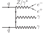
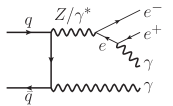
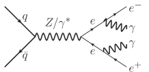
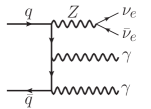
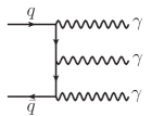
Figure 1: Examples of topologies of Feynman diagrams contributing to the different processes at tree level. Top row: $pp\to Z\gamma\gamma$ + X including $Z$ decays into a pair of charged leptons. Bottom row: $pp\to Z\gamma\gamma$ + X including $Z$ decays into a pair of neutrinos (left) and $pp\to\gamma\gamma\gamma$ + X (right).

We calculate all contributions up to order $\alpha_{s}\alpha^{4}$ to the processes (1) and (2) in the limit of massless fermions. In Fig. 1, we show examples of Feynman diagrams appearing in our calculation. The different possibilities for the decay into charged leptons are depicted in the top row. Either all three vector bosons can be attached to the quark line (left), or one (middle) or both (right) photons are radiated off the charged leptons. In total, 40 different Feynman diagrams appear at leading order. To improve the speed of the calculation, we use the technique of “leptonic tensors” as described in Ref. Jager:2006zc . Invariant subparts of the amplitude, namely the decays of the $Z$ and virtual photons, are computed independently of the rest of the amplitude and only once per phase-space point. The result can then be easily reused when calculating the matrix elements, which greatly reduces the required computation time. Up to permutations of the vector bosons, only the diagram on the bottom left of Fig. 1 can appear at leading order for $Z$ decays into a pair of neutrinos. Hence, the photons are always radiated off the quark line.

The process (3) is correspondingly calculated up to order $\alpha_{s}\alpha^{3}$. Up to permutations of the photons, only the Feynman diagram depicted in the lower right of Fig. 1 contributes at leading order.

To compute all these matrix elements, we use the helicity formalism of Ref. Hagiwara:1985yu . Contributions from virtual diagrams, which interfere with the tree-level diagrams, and from real emission occur at NLO QCD. Both are infrared divergent, but the sum of them does not contain any infrared divergences according to the Kinoshita-Lee-Nauenberg (KLN) theorem Kinoshita:1962ur . We achieve this cancellation in a numerically stable way by using the Catani-Seymour dipole subtraction method Catani:1996vz , which analytically extracts the divergences which are then canceled against the virtual ones. Part of the initial-state collinear singularities is factored into the parton-distribution functions, giving rise to additional so-called “finite collinear terms”. The NLO real corrections are obtained from the LO diagrams by attaching a gluon to the quark line in every possible way. This gluon can then be either a final-state particle, radiated off the quark line, or an initial-state one splitting into a quark–anti-quark pair. For the $Z_{\ell}\gamma\gamma$ case there are 120 Feynman diagrams for each possibility. Hence, using leptonic tensors is particularly useful in this case.

We obtain the virtual NLO QCD corrections by inserting gluon lines into the diagrams of Fig. 1 in every possible way. This yields loop diagrams with up to five external legs, i.e. pentagon diagrams. The occurring five-point integrals are solved using the prescription given in Ref. Denner:2002ii , which does not need any inverse Gram determinants, with the setup of Ref. Campanario:2011cs . For loop integrals up to the box level, we use Passarino-Veltman reduction Passarino:1978jh . There we circumvent the explicit calculation of inverse Gram determinants numerically by solving a system of linear equations, which leads to a more stable behavior close to the critical regions. For all loop contributions, the full virtual corrections

$$M_{V}=\widetilde{M}_{V}+\ \frac{\alpha_{S}}{4\pi}\ C_{F}\ \left(\frac{4\pi\mu^{2}}{Q^{2}}\right)^{\epsilon}\ \Gamma{(1+\epsilon)}\ \left[-\frac{2}{\epsilon^{2}}-\frac{3}{\epsilon}-8+\frac{4\pi^{2}}{3}\right]\ M_{B},$$ (4)

factorize into a part proportional to the Born amplitude $M_{B}$ and an infrared-finite remainder, $\widetilde{M}_{V}$. $Q$ denotes the partonic center-of-mass energy, i.e. the invariant mass of the photons and, for the $Z\gamma\gamma$ case, the leptons. We note that for diagrams where only a single vector boson is attached to the quark line (top right diagram of Fig. 1), the virtual corrections completely factorize to their corresponding Born matrix element, i.e. they do not contribute to $\widetilde{M}_{V}$. The finite remainders for all virtual corrections to two-boson amplitudes (top center diagram of Fig. 1) are called “virtual-box” and to all three vector bosons attached to the quark line “virtual-pentagons” in the following. They were computed with the method described in Ref. Campanario:2011cs . To test the gauge invariance of the total $Z\gamma\gamma$ amplitude, we write the polarization vector of the $Z$ as $\epsilon_{Z}^{\mu}=x_{Z}q_{Z}^{\mu}+\tilde{\epsilon}_{Z}^{\mu}$, where the last part simply denotes the remaining piece. Due to the structure of the amplitude, we cannot shift any contributions from pentagons to boxes, as has been done in other triboson processes Hankele:2007sb ; Campanario:2008yg ; Bozzi:2009ig ; Bozzi:2010sj . Still, individual pentagon amplitudes change significantly depending on the value of $x_{Z}$. We have verified that their sum nevertheless stays unchanged.

Isolated photons in the final state require particular care for the real emission part. Collinear emission of a photon from a massless quark leads to additional infrared divergences. Applying a naive separation cut between these two particles is not possible, however, since this would restrict the phase-space of the final-state parton and therefore spoil the cancellation of divergences between virtual and real part. In this article, we solve the problem by imposing a particularly crafted cut Frixione:1998jh between final-state parton (quark or gluon) $i$ and photon $\gamma_{j}$

$$p_{T_{i}}\leq p_{T_{\gamma_{j}}}\frac{1-\cos R_{\gamma_{j}i}}{1-\cos\delta_{0}}\text{\quad or\quad}R_{\gamma_{j}i}>\delta_{0}\ ,$$ (5)

where $j$ runs over all final-state photons and $\delta_{0}$ is a fixed separation parameter. This cut allows the parton to be arbitrarily close to the photon, as long as its momentum vanishes simultaneously. This procedure avoids electroweak divergences, keeping at the same time the QCD pole of the real part intact.

We have performed several cross checks to verify that our calculation is correct. First, all tree-level matrix elements have been compared against corresponding code generated by MadGraph Stelzer:1994ta . We find an agreement at the level of the machine precision, i.e. at least 14 significant digits. Furthermore, we have compared the integrated cross sections of all leading-order processes as well as those with an additional jet against MadEvent and Sherpa Sherpa:09 . For the triple photon process, internal technical cuts in these programs make the comparison difficult when we impose rather loose cuts on the photons. Therefore, we have performed an additional cross check with FeynArts FA /FormCalc FC /HadCalc HC for this instance. In all cases, we find an excellent agreement between the codes below the per mill level, compatible with the integration error. Also, the implementation of the Catani-Seymour subtraction scheme has been checked. We have tested that the large contributions from the true real-emission diagrams are canceled by the corresponding dipole terms once we approach the soft or collinear regions. Additionally, we have verified that finite contributions appearing in the subtraction scheme can be shifted between the virtual and the real part without affecting the total result. Furthermore, for the virtual corrections we employ a gauge test for each phase-space point.

III Numerical Results

We obtain numerical results from an NLO Monte Carlo program based on the structure of the VBFNLO program package Arnold:2008rz . In the electroweak sector, we take the masses of the $W$ and $Z$ boson as well as the Fermi constant as input. We then use tree-level relations to calculate the weak mixing angle and the electromagnetic coupling from these. As numerical values we hence use

$$m_{W}=80.398\ \mathrm{GeV} \sin^{2}{(\theta_{W})}=0.22264$$

$$m_{Z}=91.1876\ \mathrm{GeV} \alpha^{-1}=132.3407$$

$$G_{F}=1.16637\cdot 10^{-5}\ \mathrm{GeV}^{-2}\;.$$ (6)

We do not consider any effects arising from top quarks. All other quarks are considered to be massless. As parton distribution functions we use the CTEQ6L1 set at LO Pumplin:2002vw and the CT10 set with $\alpha_{S}(m_{Z})=0.118$ at NLO Lai:2010vv . For both sets, we use five active flavors as initial-state quarks and in the renormalization group running of the strong coupling constant. As central value for the factorization and renormalization scale, we take the invariant mass of all uncolored particles, i.e.

$$\mu_{F}=\mu_{R}=\mu_{0}=\begin{cases}m_{Z\gamma\gamma}\equiv\sqrt{(p_{\ell_{1}/\nu_{1}}+p_{\bar{\ell}_{1}/\bar{\nu}_{1}}+p_{\gamma_{1}}+p_{\gamma_{2}})^{2}}&\text{for $Z\gamma\gamma$ and}\\ m_{\gamma\gamma\gamma}\equiv\sqrt{(p_{\gamma_{1}}+p_{\gamma_{2}}+p_{\gamma_{3}})^{2}}&\text{for $\gamma\gamma\gamma$.}\end{cases}$$ (7)

To take into account typical requirements of the experimental detectors, we impose the following set of minimal cuts on the transverse momentum and rapidity of the final-state charged leptons and photons

$$p_{T_{\gamma}} >20\ \mathrm{GeV} p_{T_{\ell}} >20\ \mathrm{GeV} |y_{\gamma}| <2.5 |y_{\ell}| <2.5\ .$$ (8)

Furthermore, photons, charged leptons and jets need to be well-separated in phase space, so they can be identified as separate objects in the detector. Also, divergences from collinear photons need to be eliminated by cuts. Hence, we use additionally

$$R_{\ell\ell} >0.3 R_{\gamma\gamma} >0.4 R_{\ell\gamma} >0.4 R_{j\ell} >0.4 R_{j\gamma} >0.7 m_{\ell^{+}\ell^{-}} >15\ \mathrm{GeV}\ ,$$ (9)

where the last requirement removes the singularity from a virtual photon splitting into a pair of oppositely charged leptons, when the invariant mass of the lepton pair becomes small. For the purpose of these cuts, a jet is defined as a final-state gluon or quark with $p_{T_{j}}>30$ GeV and $|y_{j}|<4.5$. Furthermore, we impose the restriction defined in Eq. (5) with the parameter $\delta_{0}=0.7$, which eliminates electroweak divergences between final-state quarks or gluons and photons collinear to them.

LHC	LO [fb]		NLO [fb]		K-factor
$~{}\sigma("Z\gamma\gamma"\to e^{+}e^{-}\gamma\gamma)$
$~{}~{}p_{T{\gamma(\ell)}}>20(20)$ GeV	03.2080		04.8770		1.52
$~{}~{}p_{T{\gamma(\ell)}}>30(20)$ GeV	00.9987		01.5650		1.57
$~{}\sigma("Z\gamma\gamma"\to\nu\bar{\nu}\gamma\gamma)$
$~{}~{}p_{T{\gamma}}>20$ GeV	02.9050		04.5100		1.55
$~{}~{}p_{T{\gamma}}>30$ GeV	01.1870		01.9060		1.61
$~{}\sigma("\gamma\gamma\gamma")$
$~{}~{}p_{T{\gamma}}>20$ GeV	22.1700		58.5700		2.64
$~{}~{}p_{T{\gamma}}>30$ GeV	06.9070		16.4900		2.39

Table 1: Total cross sections at the LHC for $pp\to Z\gamma\gamma+X$ with decays into charged leptons and neutrinos, and for $pp\to\gamma\gamma\gamma$. We show results for two sets of cuts at LO, NLO, and the associated K-factor. Relative statistical errors of the Monte Carlo are below $10^{-3}$.

Tevatron	LO [fb]		NLO [fb]		K-factor
$~{}\sigma("Z\gamma\gamma"\to e^{+}e^{-}\gamma\gamma)$
$~{}~{}p_{T{\gamma(\ell)}}>10(10)$ GeV	11.8100		16.3700		1.39
$~{}~{}p_{T{\gamma(\ell)}}>20(10)$ GeV	01.5680		02.2260		1.42
$~{}\sigma("Z\gamma\gamma"\to\nu\bar{\nu}\gamma\gamma)$
$~{}~{}p_{T\gamma}>10$ GeV	02.4210		03.5340		1.46
$~{}~{}p_{T\gamma}>20$ GeV	00.5820		00.8492		1.46
$~{}\sigma("\gamma\gamma\gamma")$
$~{}~{}p_{T\gamma}>10$ GeV	40.6700		84.2000		2.07
$~{}~{}p_{T\gamma}>20$ GeV	06.0080		10.2800		1.71

Table 2: Total cross sections at the Tevatron for $pp\to Z\gamma\gamma+X$ with decays into charged leptons and neutrinos, and for $pp\to\gamma\gamma\gamma$. We show results for two sets of cuts at LO, NLO, and the associated K-factor. Relative statistical errors of the Monte Carlo are below $10^{-3}$.

In Table 1, we present results for the integrated cross section of $Z\gamma\gamma$ and $\gamma\gamma\gamma$ production at the LHC with a center-of-mass energy of $14$ TeV at the central scale $\mu_{0}$. Besides our standard set of cuts in Eqs. (8) and (9), we also show results with a modified cut on the transverse momentum of the photon of 30 GeV. The results for the Tevatron with its center-of-mass energy of $1.96$ TeV are denoted in Table 2. Here, we have reduced the cut on ${p_{T}}_{\ell}$ to 10 GeV, and besides the standard value of 20 GeV also give results for ${p_{T}}_{\gamma}$ larger than 10 GeV. In all cases, we consider only a single generation of charged leptons or neutrinos in the final state.

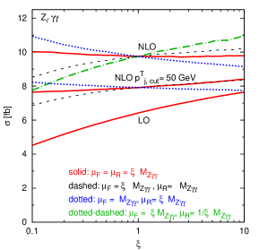
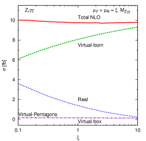
Figure 2: Left: Scale dependence of the total LHC cross section for $pp\to Z\gamma\gamma+X\to\ell^{+}\ell^{-}\gamma\gamma+X$ at LO and NLO within the cuts of Eqs. (8, 9). The factorization and renormalization scales are together, inversely or independently varied in the range from $0.1\cdot\mu_{0}$ to $10\cdot\mu_{0}$. We show NLO curves without and including an additional veto on ${p_{T}}_{j}$ of 50 GeV. Right: Same as in the left panel without jet veto, but for the different NLO contributions at $\mu_{F}=\mu_{R}=\xi\mu_{0}$ with $\mu_{0}=m_{Z\gamma\gamma}$.

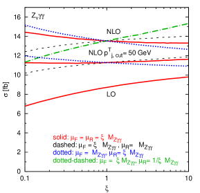
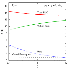
Figure 3: Left: Scale dependence of the total LHC cross section for $pp\to Z\gamma\gamma+X\to\nu\bar{\nu}\gamma\gamma+X$ at LO and NLO within the cuts of Eqs. (8, 9). The factorization and renormalization scales are together, inversely or independently varied in the range from $0.1\cdot\mu_{0}$ to $10\cdot\mu_{0}$. We show NLO curves without and including an additional veto on ${p_{T}}_{j}$ of 50 GeV. Right: Same as in the left panel without jet veto, but for the different NLO contributions at $\mu_{F}=\mu_{R}=\xi\mu_{0}$ with $\mu_{0}=m_{Z\gamma\gamma}$.

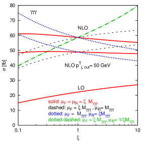
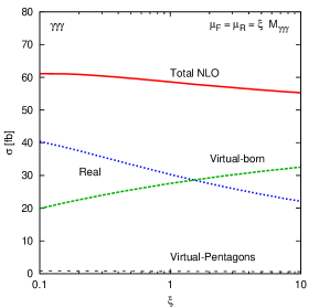
Figure 4: Left: Scale dependence of the total LHC cross section for $pp\to\gamma\gamma\gamma+X$ at LO and NLO within the cuts of Eqs. (8, 9). The factorization and renormalization scales are together, inversely or independently varied in the range from $0.1\cdot\mu_{0}$ to $10\cdot\mu_{0}$. We show NLO curves without and including an additional veto on ${p_{T}}_{j}$ of 50 GeV. Right: Same as in the left panel without jet veto, but for the different NLO contributions at $\mu_{F}=\mu_{R}=\xi\mu_{0}$ with $\mu_{0}=m_{\gamma\gamma\gamma}$.

From hereon, we will restrict ourselves to results for the LHC. Additionally, we now sum over both electrons and muons in $Z_{\ell}\gamma\gamma$ and over all three neutrino generations in $Z_{\nu}\gamma\gamma$. In Figs. 2 and 3, we show the dependence of the cross section on the factorization and renormalization scale for the $Z\gamma\gamma$ process with decays into charged leptons and neutrinos, respectively. We vary both scales together, independently and inversely, such that when one scale is increased, the other one decreases by the same factor, in the range

$$\mu_{F},\mu_{R}=\xi\cdot\mu_{0}\quad(0.1<\xi<10)\ ,$$ (10)

where the central scale $\mu_{0}$ has been given in Eq. (7). The corresponding plot for the $\gamma\gamma\gamma$ process is displayed in Fig. 4. In all cases, we also show results where we have applied an additional veto on jets with ${p_{T}}_{j}>50\text{ GeV}$. This results in smaller renormalization scale variations, but the principal shapes of the different curves are not affected. We observe that for all processes, the NLO corrections are much larger than estimated by a scale variation of the LO result. The respective K-factors at the central scale are 1.52 and 1.55 for $Z\gamma\gamma$ decaying into charged leptons and into neutrinos, and 2.64 for $\gamma\gamma\gamma$. We observe that the NLO cross section typically rises with the factorization scale and decreases with the renormalization scale. This leads to cancellations for the combined scale dependence which can yield a very flat behavior, as can be seen for example in Fig. 2. In contrast, when we vary the two scales inversely, the variations add up and lead to a rather significant dependence. This almost flat behavior is therefore accidental, and should not be considered as a very small remaining scale uncertainty.

On the right-hand side of Figs. 2, 3 and 4, we show the individual contributions to the unvetoed NLO cross section for the different processes as function of the combined factorization and renormalization scale. Both the real-emission part, which contains the true real-emission contribution, the dipole terms from the Catani-Seymour subtraction scheme and the finite collinear terms, as well as the virtual part proportional to the Born matrix element exhibit a strong scale dependence, which partly cancels in the sum. For the $Z\gamma\gamma$ process, the bulk of the contribution is given by the virtual part, while for $\gamma\gamma\gamma$ it is evenly distributed between the two. This is due to the higher average partonic center-of-mass energy for $Z\gamma\gamma$, which reduces the initial-state gluon parts due to the steep fall-off of the gluon pdfs with growing energy. The pentagon finite virtual remainders, “virtual-pentagons”, defined in Eq. (4), are small in all cases. Finite box virtual remainders, “virtual-box”, exist only for the $Z_{\ell}\gamma\gamma$ process and they are small as well.

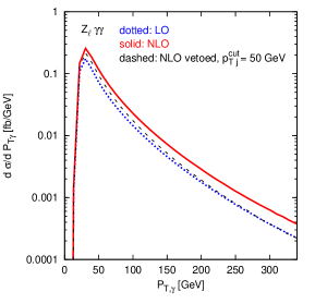
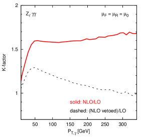
Figure 5: Left: Transverse-momentum distribution of the photon with largest transverse momentum in $Z_{\ell}\gamma\gamma$ production with $Z$ decaying into charged leptons for the LHC. We show LO (dotted blue line) and NLO cross sections without (solid red) and including (dashed black) a jet veto of 50 GeV, using the cuts of Eqs. (8, 9). Right: Associated K-factor as defined in Eq.(11) without (solid red) and including (dashed black) the jet veto.

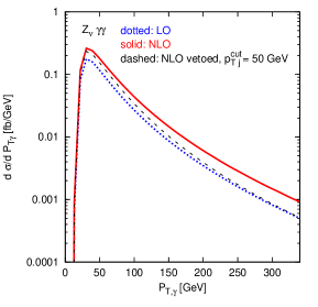
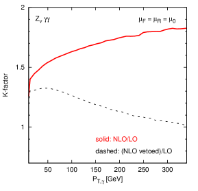
Figure 6: Left: Transverse-momentum distribution of the photon with largest transverse momentum in $Z_{\nu}\gamma\gamma$ production with $Z$ decaying into neutrinos for the LHC. We show LO (dotted blue line) and NLO cross sections without (solid red) and including (dashed black) a jet veto of 50 GeV, using the cuts of Eqs. (8, 9). Right: Associated K-factor as defined in Eq.(11) without (solid red) and including (dashed black) the jet veto.

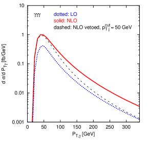
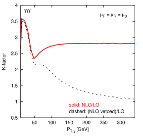
Figure 7: Left: Transverse-momentum distribution of the photon with largest transverse momentum in $\gamma\gamma\gamma$ production for the LHC. We show LO (dotted blue line) and NLO cross sections without (solid red) and including (dashed black) a jet veto of 50 GeV, using the cuts of Eqs. (8, 9). Right: Associated K-factor as defined in Eq.(11) without (solid red) and including (dashed black) the jet veto.

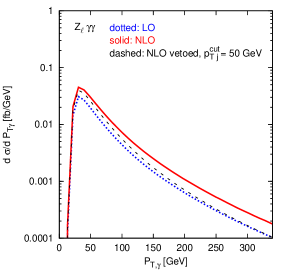
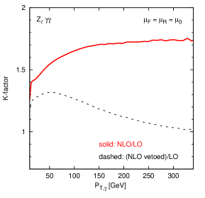
Figure 8: Left: Transverse-momentum distribution of the photon with largest transverse momentum in $Z_{\ell}\gamma\gamma$ production with $Z$ decaying into charged leptons for the LHC. We show LO (dotted blue line) and NLO cross sections without (solid red) and including (dashed black) a jet veto of 50 GeV, using the cuts of Eqs. (8, 9) and the additional cut on $m_{\ell\ell}$ given in Eq. (12). Right: Associated K-factor as defined in Eq.(11) without (solid red) and including (dashed black) the jet veto.

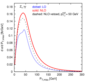
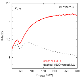
Figure 9: Left: Distribution of missing transverse momentum in $Z_{\nu}\gamma\gamma$ production with $Z$ decaying into neutrinos for the LHC. We show LO (dotted blue line) and NLO cross sections without (solid red) and including (dashed black) a jet veto of 50 GeV, using the cuts of Eqs. (8, 9). Right: Associated K-factor as defined in Eq.(11) without (solid red) and including (dashed black) the jet veto.

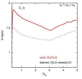
Figure 10: Left: Separation of the two photons in $Z_{\nu}\gamma\gamma$ production with $Z$ decaying into neutrinos for the LHC. We show LO (dotted blue line) and NLO cross sections without (solid red) and including (dashed black) a jet veto of 50 GeV, using the cuts of Eqs. (8, 9). Right: Associated K-factor as defined in Eq.(11) without (solid red) and including (dashed black) the jet veto.

Finally, we look at several differential distributions for all considered processes. In each figure, we show at the left-hand side the differential cross section both at LO and NLO. The latter we plot without and including an additional veto on jets with ${p_{T}}_{j}>50\text{ GeV}$. On the right-hand side, we depict the differential K-factor for both the unvetoed results and including the jet veto. It is defined as

$$K=\frac{d\sigma^{NLO}/dx}{d\sigma^{LO}/dx}\ ,$$ (11)

where $x$ denotes the considered observable.

In Figs. 5, 6 and 7, we present the transverse-momentum distributions of the photon with the largest transverse momentum for $Z_{\ell}\gamma\gamma$, $Z_{\nu}\gamma\gamma$ and $\gamma\gamma\gamma$, respectively. For each of the different processes, the K-factor for the differential distribution is not constant. Rather, we observe for the $Z\gamma\gamma$ processes a significant rise with larger transverse momenta. At small transverse momenta, the K-factor is close to the integrated results, as this is where the bulk of the cross section lies. Once we apply the additional jet veto, the K-factor instead drops to unity as the transverse momentum of the photon increases. Hence, the large differential K-factors are caused by events where the leptonic system recoils against the additional jet. For tri-photon production (Fig. 7), we observe a substantially larger K-factor for very small transverse photon momenta, where the recoil against the jet helps to fulfill the transverse-momentum cut, but is not yet large enough to trigger the possible jet veto. Once we go to large values, the K-factor is almost constant without jet veto, and gradually drops to one including it.

Furthermore, we show this distribution in Fig. 8 for $Z_{\ell}\gamma\gamma$, where we have applied the additional cut

$$m_{Z}-2\Gamma_{Z}<m_{\ell\ell}<m_{Z}+2\Gamma_{Z}$$ (12)

on the invariant mass $m_{\ell\ell}$ of the lepton pair. This cut allows us to restrict the process in such a way, that the photons are predominantly radiated off the quark lines (top left diagram of Fig. 1), which is the only possibility for $Z$ decays into neutrinos. Comparing this figure with Fig. 6, we see that the shape of the plots both for the cross sections as well as for the K-factors is almost identical. We have also checked several other distributions. Up to a global normalization constant, there are only small and negligible differences between the two. Therefore, by using this cut it is possible to extrapolate the differential rate with $Z$ decays into neutrinos from the charged-lepton rate.

In Figs. 9 and 10, we present two more distributions for the $Z\gamma\gamma$ process with decay into neutrinos. The distribution of missing transverse momentum originating from the neutrino pair is shown in Fig. 9. At LO, we see a broad distribution superimposed with a peak above $2\,{p_{T}}_{\gamma,\min}=40\text{ GeV}$, which is smeared out at NLO. This gives rise to the structure at low momenta in the K-factor, which we observe in the figure. For large missing momentum, we see again a significantly larger K-factor without any veto. With an additional jet veto of 50 GeV the K-factor drops to unity in this region.

Finally, in Fig. 10 we show the separation in the rapidity–azimuthal-angle plane between the two photons, $R_{\gamma\gamma}$, for $Z_{\nu}\gamma\gamma$ . Also here, we observe a large variation of the differential K-factor with the value of the $R_{\gamma\gamma}$ separation. Both curves without and including the additional jet veto exhibit a similar shape.

Therefore, it is necessary to calculate fully differential NLO cross sections to obtain the correct shape of the distributions. A simple rescaling of the LO result with the integrated K-factor would give large deviations.

IV Conclusions

We have calculated the NLO QCD corrections to the processes $pp,p\bar{p}\to Z\gamma\gamma+X$ with decays of the $Z$ boson into both charged leptons and neutrinos and including all off-shell effects, as well as to $pp,p\bar{p}\to\gamma\gamma\gamma+X$. These processes appear as important background in searches for new physics, for example in supersymmetric GMSB models or the latter in technicolor models.

In all cases, we obtain large corrections to the leading-order cross section. The typical size of the integrated K-factors is around 1.5 for $Z\gamma\gamma$ and 2.6 for triple-photon production. This strongly exceeds the expectations from LO scale variation, which is at the level of 10% to 16%. For an estimate of the remaining scale dependence, we vary the factorization and renormalization scale by a factor two around the central scale $\mu_{0}=m_{Z\gamma\gamma/\gamma\gamma\gamma}$ such that the product of the two scales stays constant, i.e. when one scale takes the factor two, the other has factor $\tfrac{1}{2}$ and vice versa. This gives the largest differences between $\xi=2$ and $\xi=\tfrac{1}{2}$ with changes of 9.0%, 7.5% and 18.6% for $Z_{\ell}\gamma\gamma$, $Z_{\nu}\gamma\gamma$ and $\gamma\gamma\gamma$ at NLO, respectively. For a joint variation, the difference is below 4% for all processes due to accidental cancellations.

The size of the NLO corrections exhibits a strong dependence on the observable and on different regions of phase-space. We also observe that for the processes considered in this article an additional jet veto does not flatten the differential K-factors. Hence, it is necessary to have a dedicated fully-exclusive NLO parton Monte Carlo program available. We have also studied, whether a measurement of the charged-lepton decay mode in $Z\gamma\gamma$ will allow us to predict the neutrino case. Here, we find that this works well with an additional cut, which restricts the invariant mass of the lepton pair to the region close to the $Z$ pole.

With these processes, we have completed the NLO QCD calculations of triple vector-boson production at hadron colliders including off-shell effects, Higgs resonances and leptonic decays. All these processes will be available in the next release of VBFNLO.

- (1) J. M. Campbell, J. W. Huston and W. J. Stirling, Rept. Prog. Phys. 70, 89 (2007) [arXiv:hep-ph/0611148].
- (2) The CMS Collaboration, CMS-PAS-SUS-09-004 (2009)
- (3) A. Zerwekh, C. Dib, R. Rosenfeld, Phys. Lett. B549, 154-158 (2002). [hep-ph/0207270].
- (4) A. Lazopoulos, K. Melnikov and F. Petriello, Phys. Rev. D 76 (2007) 014001 [arXiv:hep-ph/0703273].
- (5) V. Hankele and D. Zeppenfeld, Phys. Lett. B 661 (2008) 103 [arXiv:0712.3544 [hep-ph]].
- (6) F. Campanario, V. Hankele, C. Oleari, S. Prestel and D. Zeppenfeld, Phys. Rev. D 78 (2008) 094012 [arXiv:0809.0790 [hep-ph]].
- (7) T. Binoth, G. Ossola, C. G. Papadopoulos and R. Pittau, JHEP 0806 (2008) 082 [arXiv:0804.0350 [hep-ph]].
- (8) G. Bozzi, F. Campanario, V. Hankele and D. Zeppenfeld, Phys. Rev. D 81, 094030 (2010) [arXiv:0911.0438 [hep-ph]].
- (9) G. Bozzi, F. Campanario, M. Rauch, H. Rzehak, D. Zeppenfeld, Phys. Lett. B696, 380-385 (2011). [arXiv:1011.2206 [hep-ph]].
- (10) U. Baur, D. Wackeroth and M. M. Weber, PoS RADCOR2009 (2010) 067 [arXiv:1001.2688 [hep-ph]].
- (11) G. Bozzi, F. Campanario, M. Rauch, D. Zeppenfeld, Phys. Rev. D83, 114035 (2011). [arXiv:1103.4613 [hep-ph]].
- (12) J. M. Campbell, K. R. Ellis and G. Zanderighi, JHEP 0712 (2007) 056 [arXiv:0710.1832 [hep-ph]].
- (13) S. Dittmaier, S. Kallweit and P. Uwer, Phys. Rev. Lett. 100 (2008) 062003 [arXiv:0710.1577 [hep-ph]]; S. Dittmaier, S. Kallweit and P. Uwer, arXiv:0908.4124 [hep-ph].
- (14) F. Campanario, C. Englert, M. Spannowsky and D. Zeppenfeld, Europhys. Lett. 88, 11001 (2009) [arXiv:0908.1638 [hep-ph]]; F. Campanario, C. Englert, M. Spannowsky, [arXiv:1010.1291 [hep-ph]].
- (15) F. Campanario, C. Englert, S. Kallweit, M. Spannowsky and D. Zeppenfeld, JHEP 1007 (2010) 076 [arXiv:1006.0390 [hep-ph]]; F. Campanario, C. Englert, M. Spannowsky, Phys. Rev. D82, 054015 (2010). [arXiv:1006.3090 [hep-ph]].
- (16) T. Binoth, T. Gleisberg, S. Karg et al., Phys. Lett. B683, 154-159 (2010) [arXiv:0911.3181 [hep-ph]].
- (17) F. Campanario, C. Englert, M. Rauch, D. Zeppenfeld, [arXiv:1106.4009 [hep-ph]].
- (18) B. Jager, C. Oleari and D. Zeppenfeld, JHEP 0607 (2006) 015 [arXiv:hep-ph/0603177]; B. Jager, C. Oleari and D. Zeppenfeld, Phys. Rev. D 73, 113006 (2006) [arXiv:hep-ph/0604200]; G. Bozzi, B. Jager, C. Oleari and D. Zeppenfeld, Phys. Rev. D 75 (2007) 073004 [arXiv:hep-ph/0701105].
- (19) K. Hagiwara and D. Zeppenfeld, Nucl. Phys. B 274 (1986) 1; K. Hagiwara and D. Zeppenfeld, Nucl. Phys. B 313 (1989) 560.
- (20) T. Kinoshita, J. Math. Phys. 3, 650 (1962); T. D. Lee and M. Nauenberg, Phys. Rev. 133, B1549 (1964).
- (21) S. Catani and M. H. Seymour, Nucl. Phys. B 485 (1997) 291 [Erratum-ibid. B 510 (1998) 503] [arXiv:hep-ph/9605323].
- (22) A. Denner and S. Dittmaier, Nucl. Phys. B 658, 175 (2003) [arXiv:hep-ph/0212259]; A. Denner and S. Dittmaier, Nucl. Phys. B 734, 62 (2006) [arXiv:hep-ph/0509141].
- (23) F. Campanario, [arXiv:1105.0920 [hep-ph]].
- (24) G. Passarino and M. J. G. Veltman, Nucl. Phys. B 160 (1979) 151.
- (25) S. Frixione, Phys. Lett. B 429, 369 (1998) [arXiv:hep-ph/9801442].
- (26) T. Stelzer and W. F. Long, Comput. Phys. Commun. 81 (1994) 357 [arXiv:hep-ph/9401258]; F. Maltoni and T. Stelzer, JHEP 0302 (2003) 027 [arXiv:hep-ph/0208156].
- (27) T. Gleisberg, S. Hoche, F. Krauss, M. Schonherr, S. Schumann, F. Siegert and J. Winter, JHEP 0902 (2009) 007 [arXiv:0811.4622].
- (28) T. Hahn, Comput. Phys. Commun. 140, 418 (2001) [arXiv:hep-ph/0012260].
- (29) T. Hahn and M. Perez-Victoria, Comput. Phys. Commun. 118, 153 (1999) [arXiv:hep-ph/9807565]. T. Hahn and M. Rauch, Nucl. Phys. Proc. Suppl. 157, 236 (2006) [arXiv:hep-ph/0601248].
- (30) M. Rauch, arXiv:0804.2428 [hep-ph].
- (31) K. Arnold et al., Comput. Phys. Commun. 180 (2009) 1661 [arXiv:0811.4559 [hep-ph]].
- (32) J. Pumplin, D. R. Stump, J. Huston, H. L. Lai, P. Nadolsky and W. K. Tung, JHEP 0207 (2002) 012 [arXiv:hep-ph/0201195].
- (33) H. L. Lai, M. Guzzi, J. Huston, Z. Li, P. M. Nadolsky, J. Pumplin and C. P. Yuan, Phys. Rev. D 82, 074024 (2010) [arXiv:1007.2241 [hep-ph]].
- (34) J. A. M. Vermaseren, Comput. Phys. Commun. 83 (1994) 45; D. Binosi, J. Collins, C. Kaufhold and L. Theussl, Comput. Phys. Commun. 180, 1709 (2009) [arXiv:0811.4113 [hep-ph]].