Revealing a Population of Heavily Obscured Active Galactic Nuclei at $z\approx 0.5\textrm{--}1$ in the Chandra Deep Field-South

Abstract

Heavily obscured ($N_{\rm H}\gtrsim 3\times 10^{23}$ cm^-2) Active Galactic Nuclei (AGNs) not detected in even the deepest X-ray surveys are often considered to be comparably numerous to the unobscured and moderately obscured AGNs. Such sources are required to fit the cosmic X-ray background (XRB) emission in the 10–30 keV band. We identify a numerically significant population of heavily obscured AGNs at $z\approx 0.5$–1 in the Chandra Deep Field-South (CDF-S) and Extended Chandra Deep Field-South by selecting 242 X-ray undetected objects with infrared-based star formation rates (SFRs) substantially higher (a factor of 3.2 or more) than their SFRs determined from the UV after correcting for dust extinction. An X-ray stacking analysis of 23 candidates in the central CDF-S region using the 4 Ms Chandra data reveals a hard X-ray signal with an effective power-law photon index of $\Gamma=0.6_{-0.4}^{+0.3}$, indicating a significant contribution from obscured AGNs. Based on Monte Carlo simulations, we conclude that $74\pm 25\%$ of the selected galaxies host obscured AGNs, within which $\approx 95\%$ are heavily obscured and $\approx 80\%$ are Compton-thick (CT; $N_{\rm H}>1.5\times 10^{24}$ cm^-2). The heavily obscured objects in our sample are of moderate intrinsic X-ray luminosity [$\approx(0.9$–$4)\times 10^{42}$ erg s^-1 in the 2–10 keV band]. The space density of the CT AGNs is $(1.6\pm 0.5)\times 10^{-4}$ Mpc^-3. The $z\approx 0.5$–1 CT objects studied here are expected to contribute $\approx 1\%$ of the total XRB flux in the 10–30 keV band, and they account for $\approx 5$–15% of the emission in this energy band expected from all CT AGNs according to population-synthesis models. In the 6–8 keV band, the stacked signal of the 23 heavily obscured candidates accounts for $<5\%$ of the unresolved XRB flux, while the unresolved $\approx 25\%$ of the XRB in this band can probably be explained by a stacking analysis of the X-ray undetected optical galaxies in the CDF-S (a 2.5 $\sigma$ stacked signal). We discuss prospects to identify such heavily obscured objects using future hard X-ray observatories.

1. INTRODUCTION

Deep X-ray surveys have provided the most effective method of identifying reliable and fairly complete samples of Active Galactic Nuclei (AGNs) out to $z\approx 5$ (e.g., see Brandt & Hasinger 2005 for a review). The observed AGN sky density reaches $\approx 10\,000$ deg^-2 in the deepest X-ray surveys, the Chandra Deep Fields (e.g., Bauer et al., 2004; Xue et al., 2011). These X-ray point sources are largely responsible for the observed cosmic X-ray background (XRB). A significant portion ($\approx 70\textrm{--}90\%$) of the XRB in the 0.5–6 keV range has been resolved into discrete sources by Chandra and XMM-Newton (e.g., Moretti et al., 2002; Bauer et al., 2004; Hickox & Markevitch, 2006), the majority of which are AGNs with moderate X-ray obscuration ($N_{\rm H}\lesssim 3\times 10^{23}$ cm^-2; e.g., Szokoly et al. 2004; Barger et al. 2005; Tozzi et al. 2006). However, the resolved fraction of the XRB decreases toward higher energies, being $\approx 60\%$ in the 6–8 keV band and $\approx 50\%$ in the 8–12 keV band (Worsley et al., 2004, 2005). Population-synthesis models suggest that at $\approx 20$–30 keV, where the XRB reaches its peak flux (e.g., Gruber et al., 1999; Moretti et al., 2009), the unobscured or moderately obscured AGNs discovered at lower energies cannot account for the XRB flux entirely, and an additional population of heavily obscured ($N_{\rm H}\gtrsim 3\times 10^{23}$ cm^-2), or even Compton-thick ($N_{\rm H}>1.5\times 10^{24}$ cm^-2, hereafter CT), AGNs at mainly $z\approx 0$–1.5 is required. The number density of these heavily obscured AGNs is estimated to be of the same order as that of moderately obscured AGNs (e.g., Gilli et al., 2007). However, as the X-ray emission (below at least 10 keV) of such sources is significantly suppressed, only a few distant heavily obscured AGNs have been clearly identified even in the deepest X-ray surveys (e.g., Tozzi et al., 2006; Alexander et al., 2008; Georgantopoulos et al., 2009; Comastri et al., 2011; Feruglio et al., 2011), and thus a significant fraction of the AGN population probably remains undetected.

Infrared (IR) selection is a powerful tool for detecting heavily obscured AGNs that cannot be identified in the X-ray band. X-ray and UV emission absorbed by the obscuring material is reprocessed and reemitted mainly at mid-IR wavelengths (e.g., Silva et al., 2004; Prieto et al., 2010). The mid-IR emission is less affected by dust extinction than at optical or near-IR wavelengths, rendering it more suitable for identifying obscured AGNs. With the Spitzer mission (Werner et al., 2004), deep mid-IR data in multiple bands can be obtained by the Infrared Array Camera (IRAC) and Multiband Imaging Photometer (MIPS) instruments.

Various IR selection methods for obscured AGNs have been proposed. Spitzer IRAC power-law selection chooses sources whose IRAC spectral energy distributions (SEDs) follow a power law with a slope of $\alpha\leq-0.5$ ($f_{\nu}\propto\nu^{\alpha}$; e.g., Alonso-Herrero et al. 2006; Donley et al. 2007, 2010). This criterion was determined based on the average optical-to-IR spectral properties of X-ray selected QSOs (e.g., Elvis et al., 1994). It can select a relatively pure sample of AGNs with little contamination from star-forming galaxies but is generally limited to the most-luminous sources (e.g., Polletta et al., 2008). IRAC color-color selection applies color cuts in the IRAC color space to identify AGNs (e.g., Lacy et al., 2004; Stern et al., 2005). This method is based on the IRAC color properties of optically selected QSOs and AGNs, and it tends to have significant contamination from star-forming galaxies when applied to deep mid-IR data (e.g., Cardamone et al., 2008; Georgantopoulos et al., 2008; Brusa et al., 2010). IR-excess selection uses a combined UV–optical–IR color cut to identify AGNs (e.g., Dey et al., 2008; Fiore et al., 2008; Lanzuisi et al., 2009). This technique is also contaminated by star-forming galaxies (e.g., Donley et al., 2008).

Compared to the above methods, which utilize observational data directly and determine the selection criteria empirically, Daddi et al. (2007) adopted a generally different approach to find obscured AGNs. They selected candidates with significantly higher IR-based (also including the component corresponding to the transmitted UV emission; see §2.1 below for details) star formation rates (SFRs) than their UV-based (after correcting for dust extinction) SFRs. The amount of excess in the IR-based SFR is a measurement of the excess in the IR emission, which is likely caused by reprocessed emission from the dusty torus of a heavily obscured AGN. This relative IR SFR excess (ISX) selection method requires and utilizes redshift information to measure the IR excess effectively, and it appears to isolate a different IR sample from the methods above (Donley et al., 2008; Alexander et al., 2008). A few of the candidates in Daddi et al. (2007) have been reliably identified as CT AGNs (Alexander et al., 2008). The ISX sample is also contaminated by star-forming galaxies due to uncertainties in the calculation of SFRs; the heavily obscured AGN fraction in the Daddi et al. (2007) sample is estimated to be $\approx 25\%$ (Alexander et al., 2011), and the rest of the objects are likely star-forming galaxies.

In this paper, we improve the ISX selection method and utilize it to search for X-ray undetected, heavily obscured AGNs at $z\approx 0.5$–1 in the Chandra Deep Field-South (CDF-S; Giacconi et al. 2002; Luo et al. 2008; Xue et al. 2011) and Extended Chandra Deep Field-South (E-CDF-S; Lehmer et al. 2005). We choose to apply the ISX method on the CDF-S and E-CDF-S galaxy sample in this redshift range for the following reasons:

• IR-selection of heavily obscured AGNs at $z\approx 0.5\textrm{--}1$ is a poorly explored territory. Most of the previous IR selections were focused on samples at $z\approx 2$, including the Daddi et al. (2007) work. Since AGNs at $z\approx 0.5$–1 contribute significantly to the resolved XRB (e.g., Worsley et al., 2005; Gilli et al., 2007), and heavily obscured AGNs in this redshift range are expected to play a similar role in the missing fraction of the XRB (e.g., Gilli et al., 2007; Treister et al., 2009), it is of interest to study the heavily obscured population at these lower redshifts. Fiore et al. (2009) selected a sample of IR-excess sources in the COSMOS field, which included some objects at $z<1$. However, detailed studies (e.g., the AGN fraction) were not focused on this low-redshift bin. Moreover, the X-ray and IR (24 $\mu$m) flux limits in the CDF-S field are $\gtrsim 10$ times more sensitive than those in the COSMOS field (Fiore et al., 2009), allowing identification of the population of heavily obscured AGNs with lower intrinsic luminosities (which are likely more numerous). Recently, Georgakakis et al. (2010) selected a sample of 19 IR-excess sources at $z\approx 1$ in the AEGIS and GOODS-N fields, but they argued that most of those X-ray undetected candidates are not heavily obscured AGNs based on IR SED modeling.

• The ISX method is best applicable at $z\approx 0.5\textrm{--}1$. The ISX method proposed by Daddi et al. (2007) is a promising technique because of its simple physical motivation and its success in selecting identified CT AGNs at $z\approx 2$. However, the ISX method has not been applied to any other studies, partially due to its known limitations. There are two essential quantities in the ISX method, the IR-based SFR ($\textrm{SFR}_{\rm IR+UV}$) and the UV-based SFR ($\textrm{SFR}_{\rm UV,corr}$). The IR-based SFR is derived mainly from the observed Spitzer MIPS 24 $\mu$m flux using the Chary & Elbaz (2001) galaxy SED templates. It has been noted that at $z>1.4$, the IR luminosity (and thus $\textrm{SFR}_{\rm IR+UV}$) derived this way is overestimated by an average factor of $\approx 5$ (Murphy et al., 2009, 2011), leading to additional contamination from galaxies in the ISX sample. The UV-based SFR is calculated using the dust-extinction corrected UV luminosity. Daddi et al. (2007) used an empirical color-extinction relation to estimate the dust extinction. However, this correlation cannot be applied to relatively old galaxies that are intrinsically red (dominated by old stellar populations instead of being reddened), and all these galaxies were removed from the Daddi et al. (2007) sample. As AGNs tend to be hosted by massive, red galaxies (e.g., Xue et al., 2010), this limitation might significantly affect the completeness of the resulting ISX sample. Both these problems can be substantially alleviated if the ISX method is applied at lower redshifts. The 24 $\mu$m deduced IR luminosity is robust at $z\lesssim 1$ (e.g., Elbaz et al., 2010), while the dust extinction can be derived via SED fitting (e.g., Brammer et al., 2009; Reddy et al., 2010). The SED-fitting technique is reliable with the high-quality multiwavelength photometric data achievable at $z\lesssim 1$.

• The CDF-S and E-CDF-S are excellent fields in which to perform such a study. They have been covered by extensive multiwavelength photometric and spectroscopic surveys, including very deep X-ray and 24 $\mu$m exposures. The COMBO-17 (Wolf et al., 2004, 2008) and Subaru (Cardamone et al., 2010) surveys covering the entire CDF-S and E-CDF-S are particularly valuable for the determination of dust extinction via SED fitting. The 17-filter coverage of COMBO-17 between $3600$ Å and $9200$ Å and 18 medium-band coverage of Subaru between $4200$ Å and $8600$ Å are useful for distinguishing between a red dust-free galaxy and a blue dusty galaxy. Reliable photometric redshifts (photo-$z$’s) can also be obtained with the high-quality multiwavelength data available.

• We can assess the possibility of directly detecting the missing population of heavily obscured AGNs with future hard X-ray observatories. One of the science goals of several future hard X-ray missions, such as the Nuclear Spectroscopic Telescope Array (NuSTAR; Harrison et al. 2010) and ASTRO-H (Takahashi et al., 2010), is to resolve better the XRB at $\approx 10$–30 keV via detecting heavily obscured and CT AGNs directly in the distant universe. While IR-selected heavily obscured AGN candidates at $z\approx 2$ are likely below their sensitivity limits, candidates at $z\approx 0.5$–1 should be more easily detectable, and we will critically assess such possibilities.

This paper is organized as follows. We describe the multiwavelength data and ISX sample selection in §2. In §3 we present an X-ray stacking analysis of the ISX sample and estimate the heavily obscured AGN fraction among the sample via simulations. In §4, we calculate the space density of the selected heavily obscured AGNs and their contribution to the XRB. We also discuss the feasibility of detecting these ISX sources with future hard X-ray observatories. We summarize in §5. Throughout this paper, we adopt the latest cosmology with $H_{0}=70.4$ km s^-1 Mpc^-1, $\Omega_{\rm M}=0.272$, and $\Omega_{\Lambda}=0.728$ (Komatsu et al., 2011). All given magnitudes are in the AB system (e.g., Oke & Gunn, 1983) unless otherwise stated.

2. THE RELATIVE IR SFR EXCESS SAMPLE

2.1. Multiwavelength Data and Source Properties

The CDF-S is the deepest X-ray survey ever performed, having a total Chandra exposure of $\approx 4$ Ms and covering a solid angle of $\approx 460$ arcmin² (Xue et al., 2011). X-ray images in three standard bands, 0.5–8.0 keV (full band; FB), 0.5–2.0 keV (soft band; SB), and 2–8 keV (hard band; HB), along with other relevant products such as the main X-ray source catalog (740 sources) and sensitivity maps, are used in the sample creation and X-ray stacking analysis, which are discussed below and in §3. The CDF-S is flanked by the E-CDF-S, which consists of four contiguous $\approx 250$ ks Chandra observations with a total solid angle of $\approx 1100$ arcmin² (Lehmer et al., 2005). The E-CDF-S main X-ray source catalog (762 sources) is used only in the sample creation.

Mid-IR-to-optical multiwavelength data are required to calculate the IR-based and UV-based SFRs in the ISX method. The CDF-S and E-CDF-S have been covered by extensive photometric and spectroscopic surveys, and we constructed a sample of mid-IR and optically selected sources in the CDF-S and E-CDF-S region. For the mid-IR data, we used the Spitzer MIPS 24 $\mu$m source catalog from the Spitzer Far Infrared Deep Extragalactic Legacy Survey (FIDEL; M. Dickinson et al. 2011, in preparation). The FIDEL survey covers the entire CDF-S and E-CDF-S, and it has a 5 $\sigma$ limiting flux of $\approx 20$ $\mu$Jy. For the IR-to-optical data, we used the master source catalog compiled by Rafferty et al. (2011), which consists of $\approx 100\,000$ optically selected galaxies covering the entire CDF-S and E-CDF-S. The master source catalog was created based on the MUSYC catalog (Gawiser et al., 2006), the COMBO-17 catalog (Wolf et al., 2004, 2008), and the GOODS-S MUSIC catalog (Grazian et al., 2006), and it was also cross-matched to several other photometric catalogs such as the SIMPLE IRAC catalog (Damen et al., 2011) and the GALEX UV catalog (e.g., Morrissey et al., 2005) to include up to 42 bands of IR-to-UV data. Additionally, we included the 18 medium-band Subaru photometric data that have become available recently (Cardamone et al., 2010); about 80% of the sources in the master catalog have Subaru data. For our purpose of computing reliably the UV-based SFRs (requiring robust IR-to-UV SED fitting), we chose sources with relatively bright $R$-band magnitudes ($R<25$); there are $\approx 40\,000$ such objects. These sources were matched to the 24 $\mu$m sources using the likelihood-ratio matching technique described in Luo et al. (2010), resulting in 5237 matches and a false-match probability of $\approx 4\%$. For sources in the X-ray stacking samples discussed in §3, we have visually examined their IR and optical images and removed sources that are probably affected by source blending, and thus the false-match probability is negligible for those samples.

Reliable spectroscopic redshifts (spec-$z$’s; 979/5237 sources) for sources in the CDF-S and E-CDF-S were collected from the following catalogs: Le Fèvre et al. (2004), Szokoly et al. (2004), Mignoli et al. (2005), Ravikumar et al. (2007), Vanzella et al. (2008), Popesso et al. (2009), Balestra et al. (2010), and Silverman et al. (2010). If a spec-$z$ is not available for a given source, we calculated its photo-$z$ using the Zurich Extragalactic Bayesian Redshift Analyzer (ZEBRA; Feldmann et al. 2006). ZEBRA utilizes a maximum-likelihood approach to find the best-fit SED template; more details about the ZEBRA SED-fitting procedure are discussed in §3.2 of Luo et al. (2010). For the purpose of our study here, we used ZEBRA to derive photo-$z$’s and dust extinction (in terms of the extinction in the $V$ band, $A_{V}$) simultaneously using up to 60 photometric bands. We selected 99 typical PEGASE galaxy templates from Grazian et al. (2006) that span a wide range of star-formation history, and we applied intrinsic extinction in the range $A_{V}=0$–4 with an increment of 0.1 to these templates employing the Calzetti et al. (2000) extinction law. The resulting SED templates were used to fit the IR-to-UV SED data (excluding the 24 $\mu$m data) of the sources. For sources with spec-$z$’s, the redshifts were fixed at the spec-$z$ values during the SED fitting, and the values of $A_{V}$ were obtained from the best-fit templates. For the other sources, both the photo-$z$ and $A_{V}$ values were determined based on the best-fit templates. To check the quality of the photo-$z$’s, we performed another ZEBRA run of the spec-$z$ sources, setting the redshift as a free parameter, and then compared the resulting photo-$z$’s with the spec-$z$’s. The photo-$z$ accuracy was estimated using the outlier fraction and the normalized median absolute deviation ($\sigma_{\rm NMAD}$; e.g., Brammer et al. 2008; Luo et al. 2010) parameters. Outliers are defined as sources having $|\Delta z|/(1+z_{\rm spec})>0.15$, where $\Delta z=z_{\rm photo}-z_{\rm spec}$, and $\sigma_{\rm NMAD}$ is defined as

$$\sigma_{\rm NMAD}=1.48\times{\rm median}\left(\frac{|\Delta z-{\rm median}(\Delta z)|}{1+z_{\rm spec}}\right)~{}.$$ (1)

For all the spec-$z$ sources, we found an outlier fraction of 6% and $\sigma_{\rm NMAD}=0.020$. For sources in the redshift range of 0.5–1, which are of primary interest for this study, the outlier fraction is 3% and $\sigma_{\rm NMAD}=0.017$. These photo-$z$’s have comparably high quality to those recently obtained for galaxies in the CDF-S region (Cardamone et al., 2010; Dahlen et al., 2010).

We calculated the IR-based and UV-based SFRs following Bell et al. (2005),

$$\textrm{SFR}_{\rm IR+UV}=9.8\times 10^{-11}(L_{\rm IR}/L_{\sun}+L_{\rm UV}/L_{\sun})~{}~{}M_{\sun}~{}{\rm yr}^{-1},$$ (2)

and

$$\textrm{SFR}_{\rm UV,corr}=9.8\times 10^{-11}(L_{\rm UV,corr}/L_{\sun})~{}~{}M_{\sun}~{}{\rm yr}^{-1},$$ (3)

where $L_{\sun}=3.8\times 10^{33}$ erg s^-1 and $L_{\rm IR}$, $L_{\rm UV}$, and $L_{\rm UV,corr}$ are the IR, UV, and dust-extinction corrected UV luminosities, respectively. The Kroupa (2001) initial mass function was adopted here. The IR luminosity was estimated by finding an IR SED template that produces the observed 24 $\mu$m luminosity via interpolation of a library of 105 IR SEDs and then calculating the integrated 8–1000 $\mu$m luminosity for this template (Chary & Elbaz, 2001). It has been demonstrated that the IR luminosity determined this way is similar to that derived with additional longer wavelength photometric data and mid-IR spectroscopic for sources with $z\lesssim 1.4$ and $L_{\rm IR}\lesssim 3\times 10^{12}~{}L_{\sun}$ (Murphy et al., 2009, 2011). The UV luminosity was computed following $L_{\rm UV}=3.3\nu l_{\nu,2800{\rm\AA}}$ (see §3.2 of Bell et al. 2005), where the rest-frame 2800 Å monochromatic luminosity $l_{\nu,2800{\rm\AA}}$ was interpolated from the multiwavelength data. We calculated the dust-extinction correction for the UV luminosity employing the Calzetti et al. (2000) extinction law, $L_{\rm UV,corr}=10^{0.72A_{V}}L_{\rm UV}$.

As AGNs tend to reside in massive galaxies (e.g., Kauffmann et al., 2003; Brusa et al., 2009; Xue et al., 2010), we estimated stellar masses for the 5237 galaxies and used these masses to filter out low-mass objects. The stellar mass is calculated following Xue et al. (2010):

$$\log(M_{*}/M_{\sun})=\log(L_{K}/L_{\sun,K})+b_{K}(M_{B}-M_{V})+a_{K}-0.10~{},$$ (4)

where $L_{\sun,K}$ is the monochromatic $K$-band luminosity of the Sun ($L_{\sun,K}=3.6\times 10^{18}$ erg s^-1 Hz^-1), the coefficients $a_{K}=-1.390$ and $b_{K}=1.176$ are from Zibetti et al. (2009), and the rest-frame monochromatic luminosity $L_{K}$ and color $(M_{B}-M_{V})$ in the Vega system are from the SED-fitting results. All the sources have IRAC detections, and thus they all have rest-frame $K$-band coverage in the SED fitting. The normalization has been adjusted by $-0.10$ dex to account for our adopted Kroupa (2001) initial mass function. The $K$-band luminosity was used because it is $\approx 5$–10 times less sensitive to dust and stellar-population effects than optical luminosities (e.g., Bell & de Jong, 2000).

2.2. Sample Selection

We define our parent sample from the 5237 optically and 24 $\mu$m selected galaxies above with the following criteria: (1) The redshift of the source is between 0.5 and 1; there are 2037 such sources. (2) The source must have COMBO-17 or Subaru detections (in $>10$ photometric bands) to ensure robust SED fitting; there are 24 sources removed by this criterion. (3) The source has a stellar mass $M_{*}>5\times 10^{9}~{}M_{\sun}$, as AGNs tend to be hosted by massive galaxies (e.g., Kauffmann et al., 2003; Brusa et al., 2009; Xue et al., 2010); this criterion removes $\approx 25\%$ of the sources. (4) The source is not X-ray detected or overlapping with the 90% encircled-energy aperture (see §3.2 of Xue et al. 2011) of any known X-ray source; the latter criterion is to avoid any contamination from nearby X-ray sources in our X-ray stacking analysis. We used the 4 Ms CDF-S and 250 ks E-CDF-S X-ray source catalogs for this purpose (Lehmer et al., 2005; Xue et al., 2011). About 200 sources are removed by this criterion. We note that the basic source properties, such as the dust extinction, stellar mass, and UV-based SFR, were calculated based on the assumption that the optical SED is dominated by the host galaxy; this assumption is valid after we exclude the X-ray sources from the sample (e.g., see §4.6.3 of Xue et al. 2010 for further discussion).

The parent sample defined above consists of 1313 sources, about 20% of which have spec-$z$’s. The spectroscopic completeness does not have any significant dependence on the IR or optical magnitude, and it is largely limited by the spectroscopic coverage in the area; for example, $\approx 60\%$ of the sources in the GOODS-S region have spec-$z$’s. We show in Figure 1 the dust extinction ($A_{V}$) against the ratio of the IR-based ($\textrm{SFR}_{\rm IR+UV}$) and UV-uncorrected [$\textrm{SFR}_{\rm UV}=9.8\times 10^{-11}(L_{\rm UV}/L_{\sun})~{}M_{\sun}~{}{\rm yr}^{-1}$] SFRs, which is also a measure of extinction. The $A_{V}$ values derived from SED fitting can well account for the extinction in general. In Figure 2, we plot the logarithmic ratios of the IR-based and UV-based SFRs, defined as $R_{\rm SFR}=\log(\textrm{SFR}_{\rm IR+UV}/\textrm{SFR}_{\rm UV,corr})$. The distribution of $R_{\rm SFR}$ displays an excess on the positive side ($R_{\rm SFR}>0$) similar to that observed in Daddi et al. (2007) for $z\approx 2$ galaxies. Various statistical errors are present in the calculations of $\textrm{SFR}_{\rm IR+UV}$ and $\textrm{SFR}_{\rm UV,corr}$, such as the uncertainties in $L_{\rm IR}$, $L_{\rm UV}$, and $A_{V}$. These tend to make the $R_{\rm SFR}$ distribution follow approximately a Gaussian function. We mirror the negative half of the histogram to the positive side, and the combined distribution (blue histogram in Fig. 2) can be approximated by a Gaussian function with $\sigma=0.33$. We thus consider that the excess in the distribution of $R_{\rm SFR}$ is caused by galaxies hosting heavily obscured or even CT AGNs. We define ISX sources using the same criterion as in Daddi et al. (2007): $R_{\rm SFR}>0.5$. For comparison, we define IR SFR normal (ISN) sources as those having $R_{\rm SFR}<0.2$. There are 242 ISX and 736 ISN sources in the parent sample. Assuming that the intrinsic dispersion of $R_{\rm SFR}$ is Gaussian (blue histogram in Fig. 2), and that the excess IR emission is powered by a heavily obscured AGN, about 73% of the ISX sources (176 objects out of the 242 ISX sources; shaded region in Fig. 2) host such AGNs. For simple comparison, we selected X-ray detected sources in the same way from the initial 5237 sources (revising the fourth criterion above to require X-ray detection in the CDF-S or E-CDF-S source catalogs); there are 198 X-ray sources selected. Following the AGN classification scheme in §4.4 of Xue et al. (2011), including criteria for intrinsic X-ray luminosity, effective power-law photon index, and X-ray-to-optical flux ratio, we identified 155 AGNs from the X-ray sources, mostly unobscured or moderately obscured. This number is comparable to that of expected heavily obscured AGNs (176 objects) in the ISX sample, consistent with predictions from population-synthesis models (e.g., Gilli et al., 2007).

Figure 1.— The dust extinction ($A_{V}$) derived from SED fitting vs. the ratio of the IR-based ($\textrm{SFR}_{\rm IR+UV}$; Eq. 2) and UV-uncorrected [$\textrm{SFR}_{\rm UV}=9.8\times 10^{-11}(L_{\rm UV}/L_{\sun})~{}M_{\sun}~{}{\rm yr}^{-1}$] SFRs for sources in the parent sample. The stars indicate the mean $A_{V}$ values in different $\textrm{SFR}_{\rm IR+UV}/\textrm{SFR}_{\rm UV}$ bins; each bin contains 60 sources. The errors on the mean values are smaller than or comparable to the symbol size. The solid line shows the ideal dust-extinction corrections which would lead to consistent IR-based and UV-based SFRs. The SED-derived $A_{V}$ values scatter around this line; the deviation of the mean $A_{V}$ values from the ideal line at large ratios of the two SFRs is likely due to the contribution from ISX sources that still have IR excesses after dust-extinction corrections (see Fig. 2).

The ISX and ISN sources have different physical properties. The median stellar mass, IR luminosity, and IR-based SFR of the ISX sample are 2.2, 1.4, and 1.2 times those for the ISN sample, respectively, while the median UV luminosity, UV-based SFR, and $A_{V}$ of the ISX sample are 50%, 15%, and 30% those for the ISN sample. If the relative excess in the IR luminosities is contributed by underlying heavily obscured AGNs, then such objects selected by the ISX method at $z\approx 0.5$–1 appear to be hosted by massive galaxies with little dust. Since AGNs are preferentially hosted by massive galaxies (e.g., Kauffmann et al., 2003; Brusa et al., 2009; Xue et al., 2010), it is natural to find ISX sources in such galaxies. The dust extinction (in terms of $A_{V}$) applies to the entire galaxy, and a small value of $A_{V}$ does not necessarily conflict with a high absorbing column density for a heavily obscured AGN in the nucleus (e.g., Maiolino et al., 2001; Polletta et al., 2008). The finding of smaller $A_{V}$ values in the ISX sources may be a selection effect. Heavily obscured AGNs at $z\approx 0.5$–1 are numerically dominated by moderate-luminosity objects (intrinsic X-ray luminosity $\approx 10^{42}$–$10^{43}$ erg s^-1) according to population-synthesis models (e.g., Gilli et al., 2007), and sources hosted by galaxies with less dust (less IR emission from the host galaxy) will have more prominent IR excesses and are more likely to be identified by IR selection methods.

As a test of whether ISX sources are preferential hosts of obscured AGNs, we also included X-ray detected CDF-S AGNs (Xue et al., 2011) in Figure 2. There are 74 CDF-S AGNs selected from the initial 5237 sources (revising the fourth criterion above to require X-ray detection in the CDF-S source catalog). We further removed 6 luminous AGNs with $L_{0.5\textrm{--}8~{}{\rm keV}}>10^{43.7}$ erg s^-1 as the optical SEDs for such sources may be affected by AGN contamination (e.g., §4.6.3 of Xue et al., 2010). The level of intrinsic absorption was estimated by assuming an underlying X-ray power-law photon index of $\Gamma=1.8$ and using XSPEC (Version 12.5.1; Arnaud 1996) to derive the appropriate $N_{\rm H}$ value that produces the observed X-ray band ratio (defined as the ratio of count rates between the HB and SB). We consider a source to be obscured if $N_{\rm H}>10^{22}$ cm^-2; otherwise, it is unobscured or only weakly obscured. Figure 2 shows clearly that AGNs in the ISX ($R_{\rm SFR}>0.5$) region are mostly obscured (17 cases out 19), while only half of the AGNs in the ISN region are obscured. We caution that the nature of the ISX population as a whole is likely different from these X-ray detected AGNs, given the apparent difference in the IR-to-X-ray flux ratios, and thus we perform detailed X-ray studies of the ISX sample in the following section.

Figure 2.— The logarithmic ratio of $\textrm{SFR}_{\rm IR+UV}$ and $\textrm{SFR}_{\rm UV,corr}$ vs. the IR luminosity for sources in the parent sample. The filled and open dots represent sources with spec-$z$’s and photo-$z$’s, respectively. X-ray AGNs in the 4 Ms CDF-S main catalog are shown as red stars (obscured) and green squares (unobscured or weakly obscured). The classification of obscured/unobscured AGNs is based on X-ray data; see §2.2. The right panel shows the distribution of $R_{\rm SFR}$ (not counting the X-ray sources). The dashed line is the reflection of the bottom half of the histogram around $R_{\rm SFR}=0$; the resulting distribution (the blue histogram) can be approximated by a Gaussian function with $\sigma=0.33$. The horizontal dotted and dash-dotted lines indicate our criteria for defining the ISX and ISN samples, respectively. About 73% of the sources in the ISX sample (shaded area) belong to the excess population compared to the Gaussian distribution, and many of these are probably hosts of heavily obscured AGNs. The majority of the X-ray AGNs in the ISX region are obscured. [See the electronic edition of the Journal for a color version of this figure.]

3. X-RAY STACKED PROPERTIES AND COMPTON-THICK AGN FRACTION

3.1. X-ray Stacking Analysis

X-ray stacking analysis is a useful technique to obtain the average X-ray properties and probe the nature of a sample of X-ray undetected objects, and it has been used extensively in previous studies of IR-selected AGN candidates (e.g., Daddi et al., 2007; Donley et al., 2008; Fiore et al., 2009). We performed X-ray stacking of the ISX and ISN samples in the three standard X-ray bands of the 4 Ms CDF-S, FB, SB, and HB. We did not stack the ISX and ISN sources in the 250 ks E-CDF-S because the total X-ray exposure is low and no significant stacked signal can be achieved. Sources located further than 6′ from the average aim point are not included in the stacking due to sensitivity degradation at large off-axis angles (e.g., Lehmer et al., 2007; Xue et al., 2011). We visually examined the IR and optical images of the remaining ISX and ISN sources, and excluded additional 10 sources (two ISX and eight ISN sources) whose 24 $\mu$m data appear to be affected by source blending. The final ISX and ISN samples used in the stacking contain 23 and 58 sources, respectively. About 70% of these sources have spec-$z$’s. We also visually checked the X-ray images and verified that these ISX and ISN sources are not close to any bright X-ray sources which could affect the stacking results. Basic properties of the ISX and ISN sources used in the X-ray stacking analysis are listed in Table 1.

We followed a stacking procedure similar to that discussed in Steffen et al. (2007). For each source in each of the three standard bands, we calculated the total (source plus background) counts within a 3″-diameter circular aperture centered on its optical position. This extraction radius was found to produce the best signal-to-noise ratio (S/N) (e.g., Worsley et al., 2006) compared to other choices. The corresponding background counts within this aperture were determined with a Monte Carlo approach which randomly (avoiding known X-ray sources) places 1000 apertures within a 1′-radius circle of the source position to measure the mean background (e.g., Brandt et al., 2001). The total counts ($S$) and background counts ($B$) for the stacked sample were derived by summing the counts for individual sources. The net source counts are then given by $(S-B)$, and the S/N is $(S-B)/\sqrt{B}$; we note that the numbers of source and background counts are large ($>100$), and thus the S/N can be calculated using Gaussian statistics. The 3″-diameter aperture does not encircle the full point-spread function (PSF). Thus we determined an encircled-energy fraction (EEF) for each source in each band by interpolating an EEF table given the aperture radius, off-axis angle, and photon energy. The EEF table was derived from the PSF images of the main-catalog sources in the 4 Ms CDF-S generated by acis extract (AE; Broos et al. 2010) that uses the marx ray-trace simulator; PSF images at five different photon energies ($\approx 0.3$–8.5 keV) for each main-catalog source in each Chandra observation were provided by AE (see §3.2 of Xue et al. 2011). We created the EEF table by calculating the EEFs at different aperture radii, off-axis angles, and photon energies, averaged over all the observations weighted by exposure time. The EEFs calculated this way are the best representative of the real CDF-S data. The EEF in a 3″-diameter aperture has a strong off-axis angle dependence, being $\approx 95\%$ for on-axis sources, and $\approx 50\%$ for sources at a 6′ off-axis angle. The aperture correction for the stacked counts was calculated using the exposure-weighted average of the EEFs for all the sources. The effective power-law photon indices and fluxes were calculated based on the band ratios and aperture-corrected count rates using the CXC’s Portable, Interactive, Multi-Mission Simulator (PIMMS; see details in §3.3.1 of Luo et al. 2008).

The stacking results are listed in Table 2, which show statistically significant differences between the ISX and ISN samples. For the ISN sample, there is a strong detection ($10.6~{}\sigma$) in the SB, while the stacked signal is weak ($1.6~{}\sigma$) in the HB. The corresponding band ratio is $0.29\pm 0.19$ (1 $\sigma$ errors), which indicates an effective power-law photon index of $\Gamma=2.0\pm 0.6$, consistent with X-ray emission from starburst galaxies (e.g., Ptak et al., 1999). The ISX sample has a $\approx 5~{}\sigma$ detection in the SB and a $\approx 4~{}\sigma$ detection in the HB (corresponding to rest-frame $\approx 3$–14 keV), with a band ratio of $1.5_{-0.5}^{+0.6}$, corresponding to $\Gamma=0.6_{-0.4}^{+0.3}$. X-ray sources with very flat spectral slopes ($\Gamma<1$) are almost exclusively identified as heavily obscured AGNs (e.g., Bauer et al., 2004), and thus a significant contribution from obscured AGNs is required to produce this kind of hard X-ray signal for the ISX sample. We note that the ISN sample may still contain a fraction of low-luminosity AGNs with soft X-ray spectra comparable to those of star-forming galaxies (e.g., González-Martín et al., 2006, 2009). These AGNs are generally unobscured and are not of primary interest to this study. In Figure 3, we show the adaptively smoothed stacked images for the ISX and ISN samples. It is clear that the ISX sample has a much harder X-ray signal than the ISN sample. The difference between the ISX and ISN samples is also apparent via comparison of their fluxes; the ISX SB flux is $\approx 40\%$ smaller than the ISN SB flux, while the ISX HB flux is $\approx 5$ times higher than the ISN HB flux.

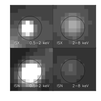
Figure 3.— The adaptively smoothed stacked images for the ISX and ISN samples. The left panels are for the SB, and the right panels are for the HB. The images were adaptively smoothed with a minimal significance (S/N) of 2.5 $\sigma$, and have been scaled linearly with the same scaling. The black circles represent the 3″-diameter aperture used to extract photometry. It is evident that the ISX sample has a much harder stacked spectrum than the ISN sample.

3.2. Heavily Obscured AGN Fraction

The stacked X-ray signal ($\Gamma\approx 0.6$) for the ISX sample indicates the existence of embedded AGNs and is consistent with X-ray emission from heavily obscured or CT AGNs modeled with a reflection spectrum (e.g., George & Fabian, 1991; Maiolino et al., 1998) or a spectrum from a toroidal reprocessor (Murphy & Yaqoob, 2009). However, we cannot derive the average AGN properties using the stacked signal directly, as the ISX sources have a range of redshifts and the sample is likely contaminated by star-forming galaxies (see, e.g., Fig. 2). We thus performed Monte Carlo simulations to assess the fraction of heavily obscured AGNs/CT AGNs in the sample, using a procedure refined from that discussed in Fiore et al. (2009). For a given AGN fraction, we ran 10 000 simulations to estimate the expected X-ray emission from both the star-forming and AGN activities of the sample, and we then compared the average simulated results to the observed stacked signal.

3.2.1 Simulation for the IR SFR Normal Sample

We first used the ISN sample (58 star-forming galaxies) to test our simulation method. For star-forming galaxies, a number of studies have found an approximately linear correlation between the SFR and rest-frame 2–10 keV X-ray luminosity $L_{\rm 2\textrm{--}10,gal}$ (e.g., Bauer et al., 2002; Ranalli et al., 2003). However, later studies have pointed out that the X-ray–SFR correlation is likely to have significant scatter due to the fact that SFR only relates to the population of relatively young high-mass X-ray binaries (HMXBs), and the older population of low-mass X-ray binaries (LMXBs) likely relates to the galaxy stellar mass (e.g., Colbert et al., 2004; Persic & Rephaeli, 2007). Therefore, we adopted the most recent relation presented in Lehmer et al. (2010), which considers the correlation of $L_{\rm 2\textrm{--}10,gal}$ with both the SFR and stellar mass,

$$L_{\rm 2\textrm{--}10,gal}=\alpha M_{*}+\beta\textrm{SFR}~{},$$ (5)

where $\alpha=2.33\times 10^{29}$ erg s^-1 $M_{\sun}^{-1}$ and $\beta=1.62\times 10^{39}$ erg s^-1 ($M_{\sun}$ yr^-1)^-1; here $\alpha$ has been increased by a factor of 2.6 to account for the average difference between stellar masses calculated in this work and Lehmer et al. (2010). Ideally, the two SFRs for a given ISN galaxy, $\textrm{SFR}_{\rm IR+UV}$ and $\textrm{SFR}_{\rm UV,corr}$, should be equal to each other. We consider that the Gaussian spread in $R_{\rm SFR}$ for ISN galaxies shown in Figure 2 is caused by uncertainties in the two SFRs, and the intrinsic SFR is estimated as $\log(\textrm{SFR})=[\log(\textrm{SFR}_{\rm IR+UV})+\log(\textrm{SFR}_{\rm UV,corr})]/2$. The corresponding 2–10 keV X-ray luminosity was then derived from Equation 5, also including a random Gaussian dispersion of 0.34 dex (Lehmer et al., 2010) to account for the scatter of that relation.

We assumed an X-ray power-law photon index of $\Gamma=2.0$ (given the stacking results) and no intrinsic absorption for the star-forming galaxies, and then converted the predicted 2–10 keV X-ray luminosity to the observed SB and HB fluxes using the individual redshifts of the sources. As none of the ISN sources is individually X-ray detected, we required that the simulated X-ray fluxes in the SB and HB of each source do not exceed the sensitivity limits at the source position. The X-ray sensitivity limits are derived following Xue et al. (2011), by calculating the minimum flux at each pixel (converted from the minimum number of counts) required for detection under the catalog source-detection criteria. We added a small Gaussian dispersion of 0.1 dex to the sensitivity limits to account for statistical fluctuations (estimated using the few CDF-S X-ray sources with fluxes below the nominal sensitivity limits). If the simulated X-ray fluxes are greater than the sensitivity limits, we made another random generation of the source properties (in this case, only Eq. 5 and the sensitivity limits have random scatters). The expected SB and HB counts were calculated given the exposure time, flux-to-count-rate conversion (using PIMMS; see Luo et al. 2008), and EEF of the source. For each simulation, net counts of every source were summed in the SB and HB as the output counts. We performed 10 000 simulations, and the average numbers of output counts are $204.2\pm 0.3$ for the SB and $57.4\pm 0.3$ for the HB (the errors are the standard errors of the mean; the 1 $\sigma$ dispersions for the average numbers of counts are both $\approx 30$), matching well with the observed stacked counts ($194.8\pm 23.1$ and $52.4\pm 33.0$). Therefore we can successfully reproduce the X-ray emission from star-forming activity with this simulation approach.

3.2.2 Simulations for the IR SFR Excess Sample

We then performed simulations for the 23 sources in the ISX sample adopting a similar approach, calculating X-ray emission from both the star-forming and AGN activities of the sample. Assuming an AGN fraction in the range of $\approx 10$–90%, the X-ray emission from the star-forming galaxies in the sample was derived following the same procedure as above.

For a source selected as an AGN, its X-ray emission and IR emission consist of both a star-formation component (host galaxy) and an AGN component. For the star-formation component, we estimated its IR-based SFR to be $\textrm{SFR}_{\rm IR,sf}=k\times\textrm{SFR}_{\rm UV,corr}$, where the factor $k$ is randomly drawn from a Gaussian function with $\sigma=0.33$ (blue histogram in Fig. 2) to account for the scatter of the calculated SFR. The intrinsic SFR of the star-formation component was then estimated as $\log(\textrm{SFR})=[\log(\textrm{SFR}_{\rm IR,sf})+\log(\textrm{SFR}_{\rm UV,corr})]/2$, and the corresponding X-ray emission was calculated. For the AGN component, the intrinsic rest-frame 2–10 keV luminosity, $L_{\rm 2\textrm{--}10,AGN}$, can be estimated from the rest-frame 6 $\mu$m luminosity of the AGN, $\nu L_{\nu,{\rm 6\mu m}}$ (e.g., Lutz et al., 2004). The relation in Lutz et al. (2004) was derived using a sample of local AGNs with the 6 $\mu$m AGN continua decomposed from the IR spectra. Here we used the luminosity-dependent version of the relation which takes into account the possible luminosity dependence (Maiolino et al., 2007; Alexander et al., 2008),

$$L_{\rm 2\textrm{--}10,AGN}=10^{4.57}\times(\nu L_{\nu,{\rm 6\mu m}})^{0.88}~{}.$$ (6)

A Gaussian dispersion of 0.4 dex was added to account for the scatter of the relation, estimated based on the range of intrinsic X-ray-to-mid-IR luminosity ratios for local AGNs (Lutz et al., 2004). We note that this relation is consistent with the X-ray-to-mid-IR luminosity ratios of a sample of X-ray selected obscured quasars (Sturm et al. 2006), suggesting that it is applicable for deriving the intrinsic luminosity of heavily obscured or CT AGNs. To derive the rest-frame 6 $\mu$m monochromatic luminosity coming from the AGN, we first computed the AGN 24 $\mu$m flux by subtracting the star-formation contribution from the observed 24 $\mu$m flux; the star-formation contribution to the 24 $\mu$m flux was estimated using the IR-based SFR ($\textrm{SFR}_{\rm IR,sf}$) above and the Chary & Elbaz (2001) IR SED templates. The residual 24 $\mu$m flux was then converted to the rest-frame 6 $\mu$m flux using the IR SED of the local CT AGN NGC 1068 (SED data from Rigopoulou et al. 1999 and Galliano et al. 2003). The observed 24 $\mu$m wavelength corresponds to rest-frame 12–16 $\mu$m for our sources, and the conversion factor to the rest-frame 6 $\mu$m flux is $\approx 0.2$–0.3.

We adopted an intrinsic photon index of $\Gamma=1.8$ for the AGN and an $N_{\rm H}$ value randomly drawn from the $N_{\rm H}$ distribution shown in Figure 7 of Gilli et al. (2007), in which about half of the AGNs are CT. The adopted $N_{\rm H}$ distribution has only a small impact on the final $N_{\rm H}$ distribution, as will be discussed later. Given the intrinsic 2–10 keV luminosity, absorption, and photon index, we estimated the observed absorbed SB and HB fluxes using the MYTorus model (Murphy & Yaqoob, 2009) implemented in XSPEC. The MYTorus model is a recently developed spectral-fitting suite for modeling the transmitted and scattered X-ray spectra from a toroidal-shaped reprocessor, and it is especially designed to treat the spectra of CT AGNs. Compared to the commonly used disk-reflection model for CT AGNs (e.g., the pexrav model in XSPEC; see Magdziarz & Zdziarski 1995), the MYTorus model is more physically motivated and takes into account absorption and scattering simultaneously. We only considered the continuum output from MYTorus for simplicity, neglecting the fluorescent iron emission lines which contribute less than 8% of the HB continuum flux. Two basic parameters describing the geometry of the model are the half-opening angle of the torus and the inclination angle (0° corresponds to a face-on observing angle). The half-opening angle was set at 37°, corresponding to a scenario where the number of obscured AGNs is four times the number of unobscured AGNs; such an obscured AGN fraction ($\approx 80\%$) for moderate-luminosity AGNs at $z\approx 1$ has been reported in several studies (e.g., Hasinger, 2008; Treister et al., 2008). We randomly chose an inclination angle between 37° and 90° (probability weighted by solid angle) for each source. Other parameters, such as the relative cross-normalizations of different components, were set at the default values (see §8.2 of the MYTorus manual). The $N_{\rm H}$ value in the MYTorus model has an upper limit of $10^{25}$ cm^-2. For column densities beyond this limit, the observed spectrum is highly geometry dependent, and the scattered flux is likely dominated by scattering in any optically thin parts of the torus, even if the effective solid angle of the optically thin gas is tiny (T. Yaqoob and K. D. Murphy 2011, private communication). The above parameterization of the model cannot reproduce the exact environment of real obscured AGNs, which could be much more complicated (e.g., Guainazzi et al., 2005; Comastri et al., 2010), but we consider it to be the best available approximation of the average properties. We then combined the emission emerging from this obscured AGN component with that from the star-formation component to derive the expected observed emission.

As for the simulations of star-forming galaxies, we required that the observed SB and HB fluxes do not exceed the sensitivity limits at the source position. We would continue randomly regenerating the source properties (e.g., $N_{\rm H}$ value) until this requirement is satisfied. This is a strong constraint on the simulated source properties, and it generally requires the AGN to be heavily obscured or CT. Finally, we converted the fluxes into counts in the extraction aperture, and added the SB and HB counts from every source as the output of a single simulation. We again performed 10 000 simulations, and the average output counts were compared to the stacking results in Table 2.

3.2.3 Simulation Results

The simulation results are shown in Figure 4, with the simulated SB and HB counts at different assumed AGN fractions. As the AGN fraction increases, the band ratio also increases and the simulated spectrum becomes harder. We note that the simulated SB photons almost exclusively originate from star-forming galaxies and AGN hosts (their star-formation components), while the HB photons are mainly from the AGNs; the increase of band ratio with AGN fraction is largely due to the increase in the HB counts. However, we did not include a soft-scattering component in the spectra of heavily obscured AGNs, which has been observed to provide significant SB emission in most of the local CT AGNs (e.g., Kinkhabwala et al., 2002; Guainazzi et al., 2009; Marinucci et al., 2011). The normalization of this component to the intrinsic power-law continuum is around 1% but has large object-to-object variations and uncertainties (e.g., Comastri et al., 2007; Gilli et al., 2007; Ueda et al., 2007), and the resulting contribution to the SB emission relative to the host-galaxy contribution depends on both this normalization and the intrinsic X-ray luminosity. Therefore the SB simulated counts should be considered lower limits, and we use only the HB results to determine the AGN fraction. As shown in Figure 4, an AGN fraction of $74\pm 25\%$ can produce the observed HB counts (see Table 3). The error on the AGN fraction was determined given the error on the observed HB counts. The $\approx 75\%$ AGN fraction is in good agreement with the fraction of extra sources (73%, shaded area) in the $R_{\rm SFR}$ distribution plot in Figure 2. For this best-fit AGN fraction, we also computed the stacked and simulated X-ray signals in several sub-bands, and the comparisons are shown in Table 3. The simulations reproduced well the stacked counts in general. The cumulative $N_{\rm H}$ distribution for the 75% of AGNs in the 10 000 simulations is displayed as an inset of Figure 4, where $\approx 95\%$ of the AGNs are heavily obscured, and $\approx 80\%$ are CT. The CT AGN fraction in the entire ISX sample is thus $\approx 60\%$. The ISX AGNs have moderate X-ray luminosities. The median intrinsic 2–10 keV luminosity derived from the simulations is $L_{\rm 2\textrm{--}10,AGN}\approx 2\times 10^{42}$ erg s^-1; this value would be $\approx 50\%$ higher if the intrinsic luminosity was calculated (Equation 6) using the observed IR flux (without subtracting the star-formation contribution). The interquartile range of the X-ray luminosities is (0.9–4)$\times 10^{42}$ erg s^-1 [(1–5)$\times 10^{42}$ erg s^-1] for the heavily obscured (CT) AGNs.

We explored how the AGN fraction could change by varying some of the assumptions in the simulations. First, we tried the commonly used disk-reflection model instead of the MYTorus model to compute obscured AGN emission. An absorbed power-law (zwabs*zpow in XSPEC) plus reflection (pexrav in XSPEC) model was used. The absorbed power-law component typically dominates in the Compton-thin ($N_{\rm H}\leq 1.5\times 10^{24}$ cm^-2) regime, and the reflection component dominates in the CT regime. We note that the pexrav model has non-negligible uncertainties on some of its parameters, such as the reflection scaling factor. For simplicity, we adopted the same parameters used in Gilli et al. (2007) to model the XRB; we assumed a cut-off energy of 200 keV, a reflection scaling factor of 0.37, and an inclination angle of 60° for the reflecting material. The hard X-ray flux produced with this model is about three times higher than that from the MYTorus model (Murphy & Yaqoob, 2009), and thus the required AGN fraction in the ISX sample is smaller. The fraction drops from $74\pm 25\%$ to $55\pm 15\%$, still indicating a substantial AGN contribution. Again, almost all ($\approx 95\%$) of the AGNs are heavily obscured. Simply increasing the $L_{\rm 2\textrm{--}10,AGN}$-to-$\nu L_{\nu,{\rm 6\mu m}}$ ratio in Equation 6 also reduces the AGN fraction. For example, if we adopt the relation used in Fiore et al. (2009), which gives an X-ray luminosity that is $\approx 0.2$ dex more luminous than ours, the resulting AGN fraction is $\approx 65\%$. The initial $N_{\rm H}$ distribution input into the simulation will affect the AGN fraction slightly. We adopted an alternative initial $N_{\rm H}$ distribution that has only $25\%$ CT AGNs, which is similar to the $N_{\rm H}$ distribution for high excitation-line galaxies in Tozzi et al. (2006). The derived AGN fraction is $60\pm 15\%$ with $\approx 90\%$ being CT. The CT AGN fraction in the entire ISX sample ($\approx 55\%$) is thus comparable to that ($\approx 60\%$) for the best-fit result above. Even in an extreme case where the initial $N_{\rm H}$ distribution has only 10% CT AGNs, an AGN fraction of $\approx 60\%$ and a CT AGN fraction of $\approx 55\%$ are still required to produce the stacked X-ray emission and satisfy the requirement that the simulated sources cannot be individually detected in the SB or HB. We note that the adopted photon index for star-forming galaxies ($\Gamma=2.0$) has little effect on the estimated AGN fraction as these galaxies produce mainly SB counts and we do not consider SB counts to be constraining.

In general, the requirement that the simulated sources cannot be individually detected places a strong constraint on the final results, and an AGN fraction of $\gtrsim 50\%$ (mostly heavily obscured) is always expected. We also caution that the simulation results were taken to be the average of 10 000 tests, and thus they (as well as the following analyses based on these results) only represent the most probable scenario of the ISX source properties and might deviate from the real source properties. We consider that this is the best available approach to probe the nature of ISX sources given the X-ray and multiwavelength data available.

Figure 4.— The average SB and HB counts of the ISX sample as a function of the AGN fraction, derived from Monte Carlo simulations. The statistical errors on the mean values are smaller than the symbol size. The SB simulated counts should be considered lower limits owing to the highly uncertain soft scattering component not included in the simulations. The two stars with error bars indicate the observed stacked SB (lower star) and HB (upper star) counts, with the best-fit AGN fraction as the $x$-axis values. The HB (SB) data point is shifted rightward (leftward) by a small amount for clarity. An AGN fraction of $74\pm 25\%$ can reproduce the observed signals. The inset panel shows the cumulative $N_{\rm H}$ distribution at this AGN fraction, with the dashed and dotted lines indicating the criteria for heavily obscured and CT AGNs. Approximately $\approx 95\%$ of the AGNs in the ISX sample are heavily obscured, and $\approx 80\%$ are CT.

4. DISCUSSION

4.1. Space Density and Contribution to the 10–30 keV XRB

Given the simulation results for the ISX sample, we can estimate the space density of heavily obscured AGNs at $z\approx 0.5$–1 and calculate their contribution to the XRB at high energies (10–30 keV). There are $16\pm 5$ ($13\pm 4$) heavily obscured (CT) AGNs expected in the X-ray stacking ISX sample. These objects are located within the central 6′-radius region of the CDF-S; the corresponding area is 0.029 deg² after excluding the regions masked by X-ray sources. We further correct the number of sources by 10% to account for the fraction removed due to blended 24 $\mu$m photometry. Therefore the sky density of heavily obscured (CT) AGNs in our ISX sample is $\approx 600$ deg^-2 ($\approx 500$ deg^-2); the corresponding space density is $(2.0\pm 0.7)\times 10^{-4}$ Mpc^-3 [$(1.6\pm 0.5)\times 10^{-4}$ Mpc^-3] given the comoving volume between redshift 0.5 and 1.

Note that there are several factors affecting the estimated space density above. The expected number of AGNs in the ISX sample may be up to $\approx 30\%$ lower if different assumptions are made in the simulations (§3.2), and thus the space density will be reduced by the same fraction. On the other hand, there is probably a small fraction of sources excluded from the parent sample with stellar mass $M_{*}\leq 5\times 10^{9}~{}M_{\sun}$ (§2.2) that also host heavily obscured AGNs. Also, the X-ray stacking ISX sample was selected in a relatively small area, and thus we have missed a few rare but intrinsically luminous AGNs, which is also suggested by the moderate IR luminosities of all the ISX sources in Table 1. Moreover, the X-ray spectra of heavily CT ($N_{\rm H}>10^{25}$ cm^-2) AGNs cannot be modeled by MYTorus and an upper limit of $10^{25}$ cm^-2 was used for the column density; if these heavily CT AGNs are present in the ISX sample, we could have overestimated their X-ray emission and thus underestimated the AGN fraction and space density. Most importantly, we define the ISX sample conservatively ($R_{\rm SFR}>0.5$) to avoid significant contamination from star-forming galaxies in the sample. There will be additional heavily obscured AGNs among those sources that are not in the ISX or ISN sample ($0.2<R_{\rm SFR}<0.5$; see §4.3 below for X-ray stacking results); the expected number is nearly comparable to that in the ISX sample given the fraction of excess sources in the distribution of $R_{\rm SFR}$ in Figure 2. Taking into account the uncertainties and incompletenesses, we expect that the true space density of heavily obscured AGNs at $z\approx 0.5$–1 is $\approx 1.5$–2 times that estimated above. In the following analyses, we still use our conservative estimation as it is difficult to determine the exact correction factor.

We show in Figure 5 the space densities of CT AGNs selected in this work and some previous studies (mainly IR based), as well as those from model predictions by Gilli et al. (2007). The CT AGN space density for the Daddi et al. (2007) CDF-S sample with $z\approx 1.4$–2.5 and $L_{\rm 2\textrm{--}10}\gtrsim 10^{43}$ erg s^-1 is estimated to be $\approx 2.6\times 10^{-4}$ Mpc^-3; the actual value is expected to be lower (e.g., Donley et al., 2008; Murphy et al., 2009) and was recently revised downward to $\approx 2\times 10^{-5}$ Mpc^-3 (Alexander et al., 2011). At lower redshift, the space density for the Fiore et al. (2009) COSMOS CT AGN sample with $z\approx 0.7$–1.2 is $(3.7\pm 1.1)\times 10^{-5}$ Mpc^-3. We are probing a different population of CT AGNs from the Fiore et al. (2009) COSMOS sample in terms of intrinsic X-ray luminosities. The interquartile range of the intrinsic 2–10 keV luminosities is (1–5)$\times 10^{42}$ erg s^-1 for the CT AGNs in our sample, while it is (3–10)$\times 10^{43}$ erg s^-1 for the Fiore et al. (2009) sample. We thus selected mainly moderate-luminosity and more typical CT AGNs; this is largely attributed to the much higher sensitivities of the mid-IR and X-ray observations in the CDF-S. On the other hand, we expect that we have missed some rare, unrepresentative objects due to the smaller area of the CDF-S. We note that the data points in various studies and model predictions have been derived with different assumptions (see, e.g., §3.2.2) and are thus not strictly comparable.

Figure 5.— Space density of CT AGNs in the ISX sample. Also shown are the CT AGN space densities in some previous IR-based studies: Daddi et al. (2007; D07), Alexander et al. (2008; A08), Fiore et al. (2008; F08), Fiore et al. (2009; F09), and Alexander et al. (2011; A11). We also include the local CT AGN density from Treister et al. (2009; T09). The redshift error bars indicate the redshift ranges of the samples, and the intrinsic 2–10 keV luminosity range of each sample is also shown. Note that the Alexander et al. (2008) and Alexander et al. (2011) data points were derived from spectroscopically (X-ray and/or IR) identified CT AGNs, the Treister et al. (2009) data point was derived based on a sample of local CT AGNs, and the other studies are based on X-ray stacking analyses of X-ray undetected candidates. The dashed curves are the predicted space densities of CT AGNs for different X-ray luminosity lower limits from the Gilli et al. (2007) population-synthesis model. Note that the various data points and model predictions have been derived with different underlying assumptions and are thus not strictly comparable.

We estimated the expected XRB flux in the 10–30 keV band provided by the heavily obscured AGNs in the ISX sample. We used the MYTorus model to calculate the emergent flux from these AGNs, given their redshifts, assumed power-law photon index ($\Gamma=1.8$), intrinsic X-ray luminosities, and column densities (the latter two quantities are from the simulation results). On average, these AGNs produce a flux of $\approx 0.6$ keV cm^-2 s^-1 sr^-1 in the 10–30 keV band, $\approx 85\%$ of which is from CT AGNs. The total XRB flux in this band is about 44 keV cm^-2 s^-1 sr^-1 (e.g., Moretti et al. 2009 and references therein). Therefore, this population of $z\approx 0.5$–1 heavily obscured (CT) AGNs selected using the ISX method is expected to contribute $\approx 1.4\%$ ($\approx 1.2\%$) of the total XRB in the 10–30 keV band. Observations have not directly resolved the XRB at energies $>10$ keV; however, theoretical predictions have been made by population-synthesis models about the contributions from unobscured, moderately obscured, and heavily obscured AGNs. For example, Gilli et al. (2007) concluded that $\approx 24\%$ of the XRB in the 10–30 keV band (the missing XRB) is produced by CT AGNs, while Treister et al. (2009) considered the total contribution from CT AGNs to be $\approx 9\%$. The predicted contribution from the CT AGNs selected here ($\approx 1.2\%$) is thus $\approx 5\%$ (Gilli et al., 2007) or $\approx 15\%$ (Treister et al., 2009) of the missing XRB in the 10–30 keV band. Given the expected properties (luminosity, redshift, column density) of the ISX sources, the Gilli et al. (2007) model predicts that $\approx 7\%$ of the missing XRB comes from such objects, agreeing well with our results. The remaining missing XRB is largely attributed to luminous ($L_{\rm 2\textrm{--}10}\approx 10^{42}$–$10^{44}$ erg s^-1) CT AGNs at $z\lesssim 1.5$ (Gilli et al., 2007); the X-ray stacking ISX sample selected here appears to have missed some of the high-luminosity objects due to the limited volume surveyed.

4.2. Resolved Fraction of the XRB by Chandra

Heavily obscured AGNs are expected also to contribute to the XRB at energies $<10$ keV, though with a smaller contributed fraction than that for the 10–30 keV band (see, e.g., Fig. 15b of Gilli et al. 2007). The XRB in the 1–8 keV band, unlike that in the 10–30 keV band, has been largely resolved into discrete sources (e.g., Bauer et al., 2004; Worsley et al., 2005; Hickox & Markevitch, 2006). With the deepest Chandra data available, the 4 Ms CDF-S, we expect to resolve the XRB further and improve our understanding of the nature of the X-ray source populations at low flux levels, including the heavily obscured population. We performed X-ray stacking analyses on the X-ray sources and optical galaxies in the CDF-S to explore the resolved XRB fraction and hidden AGN contribution to the unresolved fraction.

Measurements of the normalization of the XRB spectrum have non-negligible uncertainties and field-to-field variations; the combined uncertainty on the normalization is $\approx 10$–20% (e.g., Moretti et al., 2003; Hickox & Markevitch, 2006). Here we adopted the normalization from Hickox & Markevitch (2006), which was derived from the Chandra Deep Fields data including the 2 Ms Chandra Deep Field-North (CDF-N; Alexander et al. 2003) and 1 Ms CDF-S (Giacconi et al., 2002). The XRB has a power-law spectral slope with $\Gamma=1.4$ and a normalization of 10.9 photons s^-1 keV^-1 sr^-1 at 1 keV. X-ray stacking analyses were performed in the following energy bands: 0.5–1, 1–2, 2–4, 4–6, and 6–8 keV. For X-ray sources, we used the 740 sources in the 4 Ms CDF-S main X-ray source catalog (Xue et al., 2011). The stacking procedure was the same as that described in §3.1; to maximize the S/N ratio, a 3″-diameter circular aperture was used and the stacking was performed for the 389 sources within the inner 6′-radius area. To account properly for bright X-ray sources that have a rare occurrence in the narrow CDF-S region, we adopted the bright-end correction in Hickox & Markevitch (2006): sources brighter than $5\times 10^{-15}$ erg cm^-2 s^-1 in the SB or $1.4\times 10^{-14}$ erg cm^-2 s^-1 in the HB are removed from the stacking, and the background intensity produced by such bright sources was calculated using the number counts of X-ray sources (Hickox & Markevitch, 2006). Four sources in the SB and two in the HB are removed this way; the final stacking samples include 385 sources in the 0.5–1 and 1–2 keV bands, and 387 sources in the three $>2$ keV bands. For the optical galaxies, we chose $z$-band sources in the GOODS-S HST version r2.0z catalog (Giavalisco et al., 2004) with a 5 $\sigma$ limiting AB magnitude of $28.2$. We stacked the X-ray undetected optical galaxies in the central 6′-radius region. Galaxies within twice the 90% encircled-energy aperture radius of any known X-ray source are also removed from the stacking to avoid X-ray source contamination. There are 18 272 optical sources included in the stacking. Note that this galaxy sample contains all of the 23 sources in the X-ray stacking ISX sample.

The stacking results are shown in Figure 6. The 1 $\sigma$ errors on the stacked fluxes were calculated following Hickox & Markevitch (2006) including measurement errors and a 3% Chandra flux-calibration error. For the stacking of the X-ray sources, there is an additional Poisson error due to the limited number of sources below the bright-end flux cut (Hickox & Markevitch, 2006). Taking into account both the X-ray source contribution and bright-end correction, the resolved XRB fractions are $\approx 75\%$–80% in all the energy bands, indicating that the average photon index of the X-ray sources is $\Gamma\approx 1.4$. This is consistent with the fact that the majority of the X-ray sources in the CDF-S are obscured AGNs (e.g., Luo et al., 2010; Xue et al., 2011). For the X-ray undetected optical galaxies, significant detections are found in all the bands except the 4–6 keV band, where there is only a 1 $\sigma$ signal (corresponding to a $\approx 20\%$ chance that the signal was created by Poisson noise). We thus calculated 3 $\sigma$ upper limits on the stacked counts and resolved XRB fraction in this band. In the 6–8 keV band, the optical galaxies produced a 2.5 $\sigma$ stacked signal ($\approx 1\%$ chance of being generated by Poisson noise), responsible for $28\pm 11\%$ of the XRB. With all of the X-ray sources and galaxies considered, it appears that the XRB in the 6–8 keV band can be fully explained, though the uncertainties in the normalization and stacked signals are large (the slightly higher stacked flux than the XRB flux in this band could also be caused by cosmic variance in the CDF-S). At 1–6 keV, X-ray sources and galaxies can account for $\approx 80$–$90\%$ of the XRB. The remaining unresolved fraction is probably due to cosmic variance in the narrow CDF-S region (e.g., Bauer et al., 2004; Luo et al., 2008). It could also be partially contributed by extended X-ray sources (e.g., galaxy groups or clusters) in the CDF-S.

The 2.5 $\sigma$ stacked signal from galaxies in the 6–8 keV band ($28\pm 11\%$ of the XRB; we refer to this as the galaxy CT XRB), combined with the weak signal in the 4–6 keV band ($<6\%$ of the XRB), suggest an underlying population of heavily obscured AGNs among the X-ray undetected galaxies; emission in the 4–6 keV band is more heavily absorbed than that in the 6–8 keV band. As a subsample of the optical galaxies, the 23 ISX sources produce a stacked signal that is $0.2\pm 0.1\%$ of the total XRB flux in the 4–6 keV band; the stacked signal in the 6–8 keV band is weak (1.4 $\sigma$), and we estimated a 3 $\sigma$ upper limit that is $1.2\%$ of the total XRB. Therefore, in the 6–8 keV band, the ISX sources contribute $<5\%$ of the galaxy CT XRB. It is expected that there are some additional heavily obscured AGNs not selected with the ISX method among the optical galaxies (see §4.1 and §4.3). The number density of such objects is of about the same order of magnitude as the ISX sources.

Based on the population-synthesis model in Gilli et al. (2007), we derived that heavily obscured AGNs below the 4 Ms CDF-S sensitivity limit are responsible for $\approx 8\%$ of the XRB in the 6–8 keV band (we refer to this model prediction as the model CT XRB). This model CT XRB is only $\approx 30\%$ of the galaxy CT XRB, due to possible cosmic variance in the CDF-S and uncertainties in the model assumptions (e.g., assumptions about the spectral shape, CT AGN number density, and obscured fraction; see §9 of Gilli et al. 2007 for discussion). We also note that the Gilli et al. (2007) model does not include low-luminosity ($L_{\rm 2\textrm{--}10}\lesssim 10^{42}$ erg s^-1) AGNs. IR studies suggest that the AGN fraction in low-mass galaxies may be significantly higher than previously reported using optical spectroscopy (e.g., Goulding & Alexander, 2009). The obscured AGN fraction also increases as luminosity decreases (e.g., Hasinger, 2008). It is thus probable that low-luminosity heavily obscured AGNs have a significant stacked contribution to the galaxy CT XRB. These AGNs are faint in the X-ray band and challenging to identify even in deep Chandra observations (e.g., Goulding et al., 2010). Their IR luminosities are more likely to be dominated by host-galaxy emission and thus are difficult to detect with the ISX method (or any IR-based method).

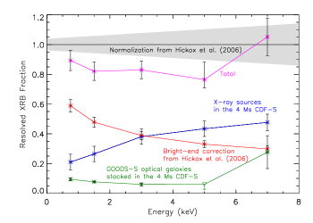
Figure 6.— Resolved fractions of the XRB in five energy bands between 0.5 and 8 keV. The total XRB intensities are from Hickox & Markevitch (2006) with uncertainties indicated by the gray region. The stacked contributions from X-ray sources in the 4 Ms CDF-S, bright-end correction, GOODS-S optical galaxies, and the sum of the above are shown as blue, red, dark green, and magenta data points, respectively. Note that the stacked signal for the optical galaxies in the 4–6 keV band did not yield a significant detection and thus a 3 $\sigma$ upper limit on the resolved fraction was calculated (triangle with a downward arrow). The upper limit was used to derive the upper error when calculating the total resolved fraction in this band. For the other data points, 1 $\sigma$ errors are shown. The contribution from the ISX objects is $<1.2\%$ in the 6–8 keV band and is not shown. [See the electronic edition of the Journal for a color version of this figure.]

4.3. Additional Samples and Subsamples

We extracted three additional X-ray stacking samples with $0.2<R_{\rm SFR}<0.5$ to test whether there are AGNs among these sources. We further break the ISX sample into two subsamples to explore how the stacking results depend on the $R_{\rm SFR}$ threshold value. The threshold cuts in $R_{\rm SFR}$ for these samples (samples A1–A5) are listed in Table 2, and they were chosen so that each sample has a similar number ($\approx 10$) of sources. We performed X-ray stacking analyses on the two subsamples and three additional samples following the same procedure as that for the ISX and ISN samples. The results are presented in Table 2. Due to limited sample sizes, these samples have less-significant detections in the HB than the ISX sample. However, the band ratios and effective photon indices for samples A1–A4 all suggest heavily obscured AGN contributions to the stacked X-ray signals. A plot of the effective photon index as a function of the average $R_{\rm SFR}$ is shown in Figure 7; in general, the larger the $R_{\rm SFR}$ threshold value (more IR excess), the harder the stacked signal. Similar behavior has also been observed by Daddi et al. (2007), and it is likely due to less contamination from star-forming galaxies at larger threshold values (see Fig. 2). Given the stacking results for these additional samples, it is not likely that the hard X-ray stacked signal of the ISX sample was produced by coincidence.

Figure 7.— The effective photon index of the stacked X-ray signal vs. the average $R_{\rm SFR}$ of the sample. Besides the ISX and ISN samples (filled circles), several additional samples (open circles) are presented with different threshold cuts in $R_{\rm SFR}$ (see Table 2). The error bars or arrows in the $x$-axis direction indicate the intervals of the $R_{\rm SFR}$ cuts. In general, as the average $R_{\rm SFR}$ increases, the stacked X-ray spectrum gets flatter, suggesting more significant contributions from heavily obscured AGNs.

4.4. Observational Prospects for Distant Heavily Obscured AGNs

A potentially straightforward way to detect distant heavily obscured or CT AGNs is via hard X-ray observations at $\approx 10$–100 keV. Several future hard X-ray missions, such as NuSTAR (planned launch year 2012; Harrison et al. 2010) and ASTRO-H (planned launch year 2014; Takahashi et al. 2010), have as one science goal to detect hard X-ray emission from distant heavily obscured AGNs. For the three typical hard X-ray bands of NuSTAR, 6–10 keV, 10–30 keV, and 30–60 keV, the expected sensitivity limits are $\approx 2\times 10^{-15}$, $2\times 10^{-14}$, and $6\times 10^{-14}$ erg cm^-2 s^-1 for a 1 Ms exposure, respectively. These flux limits are about two orders of magnitude more sensitive than those of previous missions. The ASTRO-H sensitivities are expected to be comparable to those for NuSTAR. The angular resolutions (half-power diameters) of NuSTAR and ASTRO-H are expected to be $\approx 50\arcsec$ and $\approx 1.7\arcmin$, respectively. The NuSTAR positional accuracy is expected to be $\approx 1.5\arcsec$ for strong sources. To assess if the AGNs in our ISX samples at $z\approx 0.5$–1 will be detectable, we utilized the properties for sources in the X-ray stacking ISX sample from the best-fit simulations (for the 74% AGN fraction) and the MYTorus model to calculate their expected fluxes in the NuSTAR bands. Only a tiny fraction ($\approx 0.4\%$) of the simulated sources in our 10 000 simulations have fluxes above the NuSTAR sensitivity limit in its most sensitive band (10–30 keV); this corresponds to no detected sources expected within the $16\pm 5$ heavily obscured AGNs in the X-ray stacking ISX sample (or one detectable source among all the 242 ISX objects). The median simulated flux in the 10–30 keV band ($\approx 3\times 10^{-16}$ erg cm^-2 s^-1) is about two orders of magnitude below the sensitivity limit. This result is a natural consequence of the requirement that the sources are not individually detected in the 2–8 keV band of the 4 Ms Chandra exposure; the extraordinarily high sensitivity of the 4 Ms CDF-S places a tight constraint on the intrinsic luminosities of the ISX sources and prevents them from being detected by NuSTAR. Therefore, it is not likely that NuSTAR or ASTRO-H will detect any of the ISX sources presented here. However, they will probably detect some of the X-ray selected CT AGN candidates (e.g., Tozzi et al., 2006; Comastri et al., 2011) in hard X-rays; such detections will be useful for a clear determination of the intrinsic spectral shape and power of these sources.

One other approach to identify heavily obscured or CT AGNs is via X-ray spectroscopy at relatively low energies ($<10$ keV) complemented by multiwavelength data (e.g., Polletta et al., 2006; Tozzi et al., 2006; Alexander et al., 2008, 2011; Comastri et al., 2011). The X-ray emission of these objects is characterized by a flat continuum and often a strong rest-frame 6.4 keV iron K$\alpha$ fluorescent line (e.g., Della Ceca et al., 2008; Murphy & Yaqoob, 2009). For the ISX sources presented here, spectroscopic analyses are probably not feasible due to the small number of counts expected. However, it is worth performing a further study of the X-ray selected CT AGN candidates in Tozzi et al. (2006), which were previously studied using only the 1 Ms CDF-S data. With the current 4 Ms CDF-S data and the 3 Ms XMM-Newton observations on the CDF-S, we will be able to constrain better their nature (e.g., Comastri et al., 2011). In the case of the CDF-S receiving further Chandra exposure (e.g., 10 Ms total), some ($\approx 15\%$) of the heavily obscured AGNs in the ISX sample could be detected in the HB, given the simulated properties and expected 10 Ms sensitivity.

Given the above, the majority of the heavily obscured AGNs in the ISX sample will remain undetected in the X-ray, and the few percent of the XRB at $\approx 10$–100 keV produced by these AGNs cannot be directly resolved in the near future. We note that X-ray absorption variability appears common among local Seyfert 2 galaxies (e.g., Risaliti et al., 2002), and a few sources have even exhibited CT to Compton-thin transitions (e.g., Matt et al., 2003; Risaliti et al., 2005). Therefore, a fraction of the ISX AGNs may be detectable in the future if they become less obscured due to absorption variability. Also, optical/mid-IR spectroscopy has been shown to be a promising technique for identifying distant heavily obscured AGNs, particularly when combined with sensitive X-ray constraints (e.g., Alexander et al., 2008; Gilli et al., 2010). Future optical/IR instruments such as the James Webb Space Telescope (JWST), Extremely Large Telescopes (ELTs), and Atacama Large Millimeter Array (ALMA) will provide great opportunities for detecting the remaining sources.

5. CONCLUSIONS AND FUTURE WORK

We have identified a population of heavily obscured/CT AGNs at $z\approx 0.5$–1 in the CDF-S and E-CDF-S utilizing the ISX selection method. The key points from this work are listed below:

1. We have improved the ISX method from Daddi et al. (2007) by deriving the dust extinction via SED fitting and studying sources at lower redshifts with no bias in their IR-luminosity calculation. The ISX method can be well applied to the X-ray undetected galaxies in the CDF-S region at $z\approx 0.5$–1, given the superb multiwavelength data available. The parent sample of 1313 galaxies were defined from an initial sample of 5237 optically and 24 $\mu$m selected sources in the E-CDF-S, with the requirements of selected redshift interval, excellent multiwavelength coverage, high stellar mass, and no X-ray detection (§2).

2. We have identified 242 ISX sources in the CDF-S and E-CDF-S at $z\approx 0.5$–1; these sources tend to be hosted by evolved galaxies with high stellar mass and little dust (§2.2). An X-ray stacking analysis of 23 of the objects in the central CDF-S region resulted in a very hard X-ray signal with an effective photon index of $\Gamma=0.6_{-0.4}^{+0.3}$, indicating a significant contribution from obscured AGNs (§3.1).

3. We have performed Monte Carlo simulations to estimate the AGN fraction in the ISX sample and assess the intrinsic properties of the obscured AGNs. We modeled the observed X-ray flux considering both the star-formation and AGN contributions, and we utilized the MYTorus model to treat the spectra of heavily obscured AGNs. The requirement that the sources are not individually detected in the 4 Ms CDF-S sets strong constraints on their intrinsic properties. We infer that $74\pm 25\%$ of the ISX sources are obscured AGNs, within which $\approx 95\%$ are heavily obscured and $\approx 80\%$ are CT (§3.2).

4. The heavily obscured (CT) AGNs discovered in our ISX sample have moderate intrinsic X-ray luminosities; the interquartile range of the intrinsic 2–10 keV luminosities is (0.9–4)$\times 10^{42}$ erg s^-1 [(1–5)$\times 10^{42}$ erg s^-1]. The space density of the heavily obscured (CT) AGNs is $(2.0\pm 0.7)\times 10^{-4}$ Mpc^-3 [$(1.6\pm 0.5)\times 10^{-4}$ Mpc^-3]. These heavily obscured (CT) AGNs are expected to contribute $\approx 1.4\%$ ($\approx 1.2\%$) of the total XRB flux in the 10–30 keV band. In the 6–8 keV band, the 23 ISX sources provide $<1.2\%$ of the XRB flux. The X-ray undetected optical galaxies in the CDF-S produce a 2.5 $\sigma$ stacked signal in the 6–8 keV band, accounting for $28\pm 11\%$ of the XRB flux, which is about the entire unresolved XRB fraction. The space density of the ISX AGNs and their contribution to the XRB could be increased by a factor of $\approx 1.5$–2 due to our conservative ISX definition (§4).

5. These heavily obscured or CT AGNs will probably not be detected by hard X-ray observatories under development such as NuSTAR or ASTRO-H due to their moderate intrinsic X-ray luminosities and significant obscuration. Most of the hard X-ray sources that will be detected by these facilities are likely already detected in the 4 Ms CDF-S given the extremely high sensitivity of Chandra to point sources (§4.4).

The ISX selection method presented in this paper can be applied to other survey fields with good optical-to-IR coverage, and it can be expanded to higher redshifts if the IR luminosity can be estimated reliably, e.g., combining MIPS 24 $\mu$m data with data from deep Herschel surveys at 100 and 160 $\mu$m (e.g., Shao et al. 2010). We will explore these possibilities in future work.

We acknowledge financial support from CXC grant SP1-12007A (BL, WNB, YQX), CXC grant G09-0134A (BL, WNB, YQX), NASA ADP grant NNX10AC99G (WNB), the Science and Technology Facilities Council (DMA), and ASI/INAF grant I/009/10/0 (AC, CV, RG). We are grateful to T. Yaqoob and K. D. Murphy for providing support for the MYTorus model and making available the data for our desired half-opening angle. We thank A. T. Steffen for helpful discussions. We also thank the referee for carefully reviewing the manuscript and providing helpful comments that improved this work.

Table 1List of ISX and ISN Sources in the X-ray Stacking Analysis

RA	Dec	$z$	$z$ Lower	$z$ Upper	$A_{V}$	$f_{24}$	$\log L_{\rm IR}$	$\textrm{SFR}_{\rm IR+UV}$	$\textrm{SFR}_{\rm UV,corr}$	$R_{\rm SFR}$
(1)	(2)	(3)	(4)	(5)	(6)	(7)	(8)	(9)	(10)	(11)
ISX Sample
03 32 49.61	$-$27 49 00.1	0.98	0.97	1.02	0.2	58.7	10.74	6.2	1.1	0.76
03 32 45.58	$-$27 49 36.4	0.680	$-$1.00	$-$1.00	0.9	472.3	11.46	29.5	5.0	0.77
ISN Sample
03 32 50.38	$-$27 47 07.1	0.537	$-$1.00	$-$1.00	1.9	166.5	10.86	7.7	14.1	$-0.26$
03 32 48.58	$-$27 45 04.9	0.89	0.89	0.92	1.2	121.8	11.03	12.2	12.2	$0.00$

Note. — Table 1 is presented in its entirety in the electronic edition. An abbreviated version of the table is shown here for guidance as to its form and content. The full table contains 11 columns of information for the 23 ISX sources and 58 ISN sources used in the X-ray stacking analysis. Cols. (1) and (2): The J2000 right ascension and declination of the ISX or ISN source. Cols. (3)–(5): The spec-$z$ or photo-$z$ of the source. Spec-$z$’s are denoted by having three decimal places, while photo-$z$’s with their 1 $\sigma$ confidence intervals (lower and upper bounds) were derived using ZEBRA. Col. (6): The $V$-band dust extinction derived from ZEBRA SED fitting. Col. (7): The MIPS 24 $\mu$m flux, in unites of $\mu$Jy. Col. (8): The logarithmic IR (8–1000 $\mu$m integrated) luminosity estimated based on the observed 24 $\mu$m flux, in units of solar luminosity. Cols. (9) and (10): The IR-based and UV-based SFRs, in units of $M_{\sun}$ yr^-1. Col. (11): The logarithmic ratio of the IR-based and UV-based SFRs.

Table 2Stacked X-ray Properties

				Net Source Counts			Signal-to-Noise Ratio					Flux
										Band	Effective
Sample	$N_{\rm gal}$	$z_{\rm mean}$	$t_{\rm exp}$ (Ms)	FB	SB	HB	FB	SB	HB	Ratio	$\Gamma$	SB	HB	$L_{\rm X}$
(1)	(2)	(3)	(4)	(5)	(6)	(7)	(8)	(9)	(10)	(11)	(12)	(13)	(14)	(15)
ISX ($R_{\rm SFR}>0.5$)	23	0.69	76.7	$138.8\pm 26.1$	$57.6\pm 13.9$	$78.1\pm 22.1$	6.0	4.9	3.9	$1.48_{-0.51}^{+0.63}$	$0.6_{-0.4}^{+0.3}$	4.9	36.6	8.3
ISN ($R_{\rm SFR}<0.2$)	58	0.77	193.0	$256.8\pm 40.3$	$194.8\pm 23.1$	$52.4\pm 33.0$	6.9	10.6	1.6	$0.29\pm 0.19$	$2.0\pm 0.6$	7.7	7.3	4.2
A1 ($R_{\rm SFR}>0.6$)	14	0.68	46.9	$71.5\pm 20.0$	$31.4\pm 10.6$	$39.0\pm 17.0$	4.0	3.5	2.6	$1.35_{-0.68}^{+0.90}$	$0.7_{-0.6}^{+0.5}$	4.2	28.4	6.3
A2 ($0.5<R_{\rm SFR}<0.6$)	9	0.71	29.8	$67.3\pm 16.7$	$26.1\pm 9.0$	$39.1\pm 14.1$	4.5	3.5	3.2	$1.64_{-0.73}^{+1.04}$	$0.5_{-0.6}^{+0.4}$	5.9	50.7	12.2
A3 ($0.4<R_{\rm SFR}<0.5$)	10	0.76	33.3	$45.8\pm 16.8$	$25.1\pm 9.1$	$20.7\pm 14.1$	3.1	3.2	1.8	$0.91_{-0.67}^{+0.81}$	$1.0_{-0.8}^{+0.7}$	5.6	22.7	7.1
A4 ($0.28<R_{\rm SFR}<0.4$)	11	0.69	37.7	$81.7\pm 18.5$	$47.7\pm 10.6$	$33.0\pm 15.2$	5.1	5.9	2.4	$0.76_{-0.37}^{+0.41}$	$1.2_{-0.5}^{+0.4}$	8.8	28.1	7.4
A5 ($0.2<R_{\rm SFR}<0.28$)	13	0.74	43.7	$69.4\pm 19.4$	$49.2\pm 11.2$	$19.7\pm 15.9$	4.0	5.6	1.3	$0.44_{-0.36}^{+0.37}$	$1.7\pm 0.8$	8.1	12.7	5.0

Note. — Col. (1): The X-ray stacking sample. The threshold cut in $R_{\rm SFR}$ is indicated. Col. (2): Number of sources used in the stacking. Col. (3): Mean redshift of the stacked sample. Col. (4): Total FB exposure time. Cols. (5)–(7): Stacked net source counts in the FB, SB, and HB, with 1 $\sigma$ Gaussian statistical errors. Cols. (8)–(10): Stacked signal-to-noise ratios in the FB, SB, and HB. Note that there are a few marginal detections ($<2$ $\sigma$) in the HB. Treating this kind of weak signals as detections does not affect our analyses in the paper. Col. (11): Stacked band ratio for the stacked sample, defined as the ratio of count rates between the HB and SB. The 1 $\sigma$ errors were calculated following the “numerical method” described in §1.7.3 of Lyons (1991). Col. (12): Effective photon index with 1 $\sigma$ errors for the stacked sample. Cols. (13)–(14) SB and HB fluxes for the stacked sample, in units of $10^{-18}$ erg cm^-2 s^-1. Col. (15): Rest-frame 0.5–8 keV X-ray luminosity calculated from the observed-frame 0.5–8 keV flux for the stacked sample, in units of $10^{40}$ erg s^-1. The mean redshift, observed flux, and effective power-law photon index were used in the calculation, and no assumption was made about the intrinsic absorption.

Table 3Comparison of Stacked and Simulated Counts for the ISX Sample

Band (keV)	Stacked Counts	Simulated Counts
0.5–2.0	$57.6\pm 13.9$	$57.5\pm 0.2$
2.0–8.0	$78.1\pm 22.1$	$78.9\pm 0.3$
0.5–1.0	$22.6\pm 8.6$	$19.9\pm 0.2$
1.0–2.0	$33.2\pm 11.0$	$37.6\pm 0.3$
2.0–4.0	$31.6\pm 13.3$	$36.8\pm 0.4$
4.0–8.0	$44.7\pm 17.6$	$42.1\pm 0.4$

Note. — The uncertainties for the stacked counts are 1 $\sigma$ Gaussian statistical errors. The simulated counts are the average values over the 10 000 simulations; see §3.2 for details.

References

- Alexander et al. (2003) Alexander, D. M., et al. 2003, AJ, 126, 539
- Alexander et al. (2008) —. 2008, ApJ, 687, 835
- Alexander et al. (2011) —. 2011, ApJ, in press (arXiv:1106.1443)
- Alonso-Herrero et al. (2006) Alonso-Herrero, A., et al. 2006, ApJ, 640, 167
- Arnaud (1996) Arnaud, K. A. 1996, in ASP Conf. Ser., Vol. 101, Astronomical Data Analysis Software and Systems V, ed. G. H. Jacoby & J. Barnes, 17
- Balestra et al. (2010) Balestra, I., et al. 2010, A&A, 512, 12
- Barger et al. (2005) Barger, A. J., Cowie, L. L., Mushotzky, R. F., Yang, Y., Wang, W.-H., Steffen, A. T., & Capak, P. 2005, AJ, 129, 578
- Bauer et al. (2002) Bauer, F. E., Alexander, D. M., Brandt, W. N., Hornschemeier, A. E., Vignali, C., Garmire, G. P., & Schneider, D. P. 2002, AJ, 124, 2351
- Bauer et al. (2004) Bauer, F. E., Alexander, D. M., Brandt, W. N., Schneider, D. P., Treister, E., Hornschemeier, A. E., & Garmire, G. P. 2004, AJ, 128, 2048
- Bell & de Jong (2000) Bell, E. F., & de Jong, R. S. 2000, MNRAS, 312, 497
- Bell et al. (2005) Bell, E. F., et al. 2005, ApJ, 625, 23
- Brammer et al. (2008) Brammer, G. B., van Dokkum, P. G., & Coppi, P. 2008, ApJ, 686, 1503
- Brammer et al. (2009) Brammer, G. B., et al. 2009, ApJ, 706, L173
- Brandt & Hasinger (2005) Brandt, W. N., & Hasinger, G. 2005, ARA&A, 43, 827
- Brandt et al. (2001) Brandt, W. N., Hornschemeier, A. E., Schneider, D. P., Alexander, D. M., Bauer, F. E., Garmire, G. P., & Vignali, C. 2001, ApJ, 558, L5
- Broos et al. (2010) Broos, P. S., Townsley, L. K., Feigelson, E. D., Getman, K. V., Bauer, F. E., & Garmire, G. P. 2010, ApJ, 714, 1582
- Brusa et al. (2009) Brusa, M., et al. 2009, A&A, 507, 1277
- Brusa et al. (2010) —. 2010, ApJ, 716, 348
- Calzetti et al. (2000) Calzetti, D., Armus, L., Bohlin, R. C., Kinney, A. L., Koornneef, J., & Storchi-Bergmann, T. 2000, ApJ, 533, 682
- Cardamone et al. (2008) Cardamone, C. N., et al. 2008, ApJ, 680, 130
- Cardamone et al. (2010) —. 2010, ApJS, 189, 270
- Chary & Elbaz (2001) Chary, R., & Elbaz, D. 2001, ApJ, 556, 562
- Colbert et al. (2004) Colbert, E. J. M., Heckman, T. M., Ptak, A. F., Strickland, D. K., & Weaver, K. A. 2004, ApJ, 602, 231
- Comastri (2004) Comastri, A. 2004, in Astrophysics and Space Science Library, Vol. 308, Supermassive Black Holes in the Distant Universe, ed. A. J. Barger, 245
- Comastri et al. (2007) Comastri, A., Gilli, R., Vignali, C., Matt, G., Fiore, F., & Iwasawa, K. 2007, Progress of Theoretical Physics Supplement, 169, 274
- Comastri et al. (2010) Comastri, A., Iwasawa, K., Gilli, R., Vignali, C., Ranalli, P., Matt, G., & Fiore, F. 2010, ApJ, 717, 787
- Comastri et al. (2011) Comastri, A., et al. 2011, A&A, 526, L9
- Daddi et al. (2007) Daddi, E., et al. 2007, ApJ, 670, 173
- Dahlen et al. (2010) Dahlen, T., et al. 2010, ApJ, 724, 425
- Damen et al. (2011) Damen, M., et al. 2011, ApJ, 727, 1
- Della Ceca et al. (2008) Della Ceca, R., et al. 2008, Memorie della Societa Astronomica Italiana, 79, 65
- Dey et al. (2008) Dey, A., et al. 2008, ApJ, 677, 943
- Donley et al. (2010) Donley, J. L., Rieke, G. H., Alexander, D. M., Egami, E., & Pérez-González, P. G. 2010, ApJ, 719, 1393
- Donley et al. (2008) Donley, J. L., Rieke, G. H., Pérez-González, P. G., & Barro, G. 2008, ApJ, 687, 111
- Donley et al. (2007) Donley, J. L., Rieke, G. H., Pérez-González, P. G., Rigby, J. R., & Alonso-Herrero, A. 2007, ApJ, 660, 167
- Elbaz et al. (2010) Elbaz, D., et al. 2010, A&A, 518, L29
- Elvis et al. (1994) Elvis, M., et al. 1994, ApJS, 95, 1
- Feldmann et al. (2006) Feldmann, R., et al. 2006, MNRAS, 372, 565
- Feruglio et al. (2011) Feruglio, C., Daddi, E., Fiore, F., Alexander, D. M., Piconcelli, E., & Malacaria, C. 2011, ApJ, 729, L4
- Fiore et al. (2008) Fiore, F., et al. 2008, ApJ, 672, 94
- Fiore et al. (2009) —. 2009, ApJ, 693, 447
- Galliano et al. (2003) Galliano, E., Alloin, D., Granato, G. L., & Villar-Martín, M. 2003, A&A, 412, 615
- Gawiser et al. (2006) Gawiser, E., et al. 2006, ApJ, 642, L13
- Georgakakis et al. (2010) Georgakakis, A., Rowan-Robinson, M., Nandra, K., Digby-North, J., Pérez-González, P. G., & Barro, G. 2010, MNRAS, 406, 420
- Georgantopoulos et al. (2009) Georgantopoulos, I., Akylas, A., Georgakakis, A., & Rowan-Robinson, M. 2009, A&A, 507, 747
- Georgantopoulos et al. (2008) Georgantopoulos, I., Georgakakis, A., Rowan-Robinson, M., & Rovilos, E. 2008, A&A, 484, 671
- George & Fabian (1991) George, I. M., & Fabian, A. C. 1991, MNRAS, 249, 352
- Giacconi et al. (2002) Giacconi, R., et al. 2002, ApJS, 139, 369
- Giavalisco et al. (2004) Giavalisco, M., et al. 2004, ApJ, 600, L93
- Gilli et al. (2007) Gilli, R., Comastri, A., & Hasinger, G. 2007, A&A, 463, 79
- Gilli et al. (2010) Gilli, R., Vignali, C., Mignoli, M., Iwasawa, K., Comastri, A., & Zamorani, G. 2010, A&A, 519, 92
- González-Martín et al. (2009) González-Martín, O., Masegosa, J., Márquez, I., Guainazzi, M., & Jiménez-Bailón, E. 2009, A&A, 506, 1107
- González-Martín et al. (2006) González-Martín, O., Masegosa, J., Márquez, I., Guerrero, M. A., & Dultzin-Hacyan, D. 2006, A&A, 460, 45
- Goulding & Alexander (2009) Goulding, A. D., & Alexander, D. M. 2009, MNRAS, 398, 1165
- Goulding et al. (2010) Goulding, A. D., Alexander, D. M., Lehmer, B. D., & Mullaney, J. R. 2010, MNRAS, 406, 597
- Grazian et al. (2006) Grazian, A., et al. 2006, A&A, 449, 951
- Gruber et al. (1999) Gruber, D. E., Matteson, J. L., Peterson, L. E., & Jung, G. V. 1999, ApJ, 520, 124
- Guainazzi et al. (2005) Guainazzi, M., Matt, G., & Perola, G. C. 2005, A&A, 444, 119
- Guainazzi et al. (2009) Guainazzi, M., Risaliti, G., Nucita, A., Wang, J., Bianchi, S., Soria, R., & Zezas, A. 2009, A&A, 505, 589
- Harrison et al. (2010) Harrison, F. A., et al. 2010, Proc. SPIE, 7732, 77320S
- Hasinger (2008) Hasinger, G. 2008, A&A, 490, 905
- Hickox & Markevitch (2006) Hickox, R. C., & Markevitch, M. 2006, ApJ, 645, 95
- Kauffmann et al. (2003) Kauffmann, G., et al. 2003, MNRAS, 346, 1055
- Kinkhabwala et al. (2002) Kinkhabwala, A., et al. 2002, ApJ, 575, 732
- Komatsu et al. (2011) Komatsu, E., et al. 2011, ApJS, 192, 18
- Kroupa (2001) Kroupa, P. 2001, MNRAS, 322, 231
- Lacy et al. (2004) Lacy, M., et al. 2004, ApJS, 154, 166
- Lanzuisi et al. (2009) Lanzuisi, G., Piconcelli, E., Fiore, F., Feruglio, C., Vignali, C., Salvato, M., & Gruppioni, C. 2009, A&A, 498, 67
- Le Fèvre et al. (2004) Le Fèvre, O., et al. 2004, A&A, 428, 1043
- Lehmer et al. (2010) Lehmer, B. D., Alexander, D. M., Bauer, F. E., Brandt, W. N., Goulding, A. D., Jenkins, L. P., Ptak, A., & Roberts, T. P. 2010, ApJ, 724, 559
- Lehmer et al. (2005) Lehmer, B. D., et al. 2005, ApJS, 161, 21
- Lehmer et al. (2007) —. 2007, ApJ, 657, 681
- Luo et al. (2008) Luo, B., et al. 2008, ApJS, 179, 19
- Luo et al. (2010) —. 2010, ApJS, 187, 560
- Lutz et al. (2004) Lutz, D., Maiolino, R., Spoon, H. W. W., & Moorwood, A. F. M. 2004, A&A, 418, 465
- Lyons (1991) Lyons, L. 1991, Data Analysis for Physical Science Students (Cambridge: Cambridge Univ. Press)
- Magdziarz & Zdziarski (1995) Magdziarz, P., & Zdziarski, A. A. 1995, MNRAS, 273, 837
- Maiolino et al. (2001) Maiolino, R., Marconi, A., Salvati, M., Risaliti, G., Severgnini, P., Oliva, E., La Franca, F., & Vanzi, L. 2001, A&A, 365, 28
- Maiolino et al. (1998) Maiolino, R., Salvati, M., Bassani, L., Dadina, M., della Ceca, R., Matt, G., Risaliti, G., & Zamorani, G. 1998, A&A, 338, 781
- Maiolino et al. (2007) Maiolino, R., Shemmer, O., Imanishi, M., Netzer, H., Oliva, E., Lutz, D., & Sturm, E. 2007, A&A, 468, 979
- Marinucci et al. (2011) Marinucci, A., Bianchi, S., Matt, G., Fabian, A. C., Iwasawa, K., Miniutti, G., & Piconcelli, E. 2011, A&A, 526, A36
- Matt et al. (2003) Matt, G., Guainazzi, M., & Maiolino, R. 2003, MNRAS, 342, 422
- Mignoli et al. (2005) Mignoli, M., et al. 2005, A&A, 437, 883
- Moretti et al. (2003) Moretti, A., Campana, S., Lazzati, D., & Tagliaferri, G. 2003, ApJ, 588, 696
- Moretti et al. (2002) Moretti, A., Lazzati, D., Campana, S., & Tagliaferri, G. 2002, ApJ, 570, 502
- Moretti et al. (2009) Moretti, A., et al. 2009, A&A, 493, 501
- Morrissey et al. (2005) Morrissey, P., et al. 2005, ApJ, 619, L7
- Murphy et al. (2009) Murphy, E. J., Chary, R.-R., Alexander, D. M., Dickinson, M., Magnelli, B., Morrison, G., Pope, A., & Teplitz, H. I. 2009, ApJ, 698, 1380
- Murphy et al. (2011) Murphy, E. J., Chary, R.-R., Dickinson, M., Pope, A., Frayer, D. T., & Lin, L. 2011, ApJ, 732, 126
- Murphy & Yaqoob (2009) Murphy, K. D., & Yaqoob, T. 2009, MNRAS, 397, 1549
- Oke & Gunn (1983) Oke, J. B., & Gunn, J. E. 1983, ApJ, 266, 713
- Persic & Rephaeli (2007) Persic, M., & Rephaeli, Y. 2007, A&A, 463, 481
- Polletta et al. (2008) Polletta, M., Weedman, D., Hönig, S., Lonsdale, C. J., Smith, H. E., & Houck, J. 2008, ApJ, 675, 960
- Polletta et al. (2006) Polletta, M., et al. 2006, ApJ, 642, 673
- Popesso et al. (2009) Popesso, P., et al. 2009, A&A, 494, 443
- Prieto et al. (2010) Prieto, M. A., Reunanen, J., Tristram, K. R. W., Neumayer, N., Fernandez-Ontiveros, J. A., Orienti, M., & Meisenheimer, K. 2010, MNRAS, 402, 724
- Ptak et al. (1999) Ptak, A., Serlemitsos, P., Yaqoob, T., & Mushotzky, R. 1999, ApJS, 120, 179
- Rafferty et al. (2011) Rafferty, D. A., et al. 2011, ApJ, submitted
- Ranalli et al. (2003) Ranalli, P., Comastri, A., & Setti, G. 2003, A&A, 399, 39
- Ravikumar et al. (2007) Ravikumar, C. D., et al. 2007, A&A, 465, 1099
- Reddy et al. (2010) Reddy, N. A., Erb, D. K., Pettini, M., Steidel, C. C., & Shapley, A. E. 2010, ApJ, 712, 1070
- Rigopoulou et al. (1999) Rigopoulou, D., Spoon, H. W. W., Genzel, R., Lutz, D., Moorwood, A. F. M., & Tran, Q. D. 1999, AJ, 118, 2625
- Risaliti et al. (2005) Risaliti, G., Elvis, M., Fabbiano, G., Baldi, A., & Zezas, A. 2005, ApJ, 623, L93
- Risaliti et al. (2002) Risaliti, G., Elvis, M., & Nicastro, F. 2002, ApJ, 571, 234
- Shao et al. (2010) Shao, L., et al. 2010, A&A, 518, L26
- Silva et al. (2004) Silva, L., Maiolino, R., & Granato, G. L. 2004, MNRAS, 355, 973
- Silverman et al. (2010) Silverman, J. D., et al. 2010, ApJS, 191, 124
- Steffen et al. (2007) Steffen, A. T., Brandt, W. N., Alexander, D. M., Gallagher, S. C., & Lehmer, B. D. 2007, ApJ, 667, L25
- Stern et al. (2005) Stern, D., et al. 2005, ApJ, 631, 163
- Szokoly et al. (2004) Szokoly, G. P., et al. 2004, ApJS, 155, 271
- Takahashi et al. (2010) Takahashi, T., et al. 2010, Proc. SPIE, 7732, 77320Z
- Tozzi et al. (2006) Tozzi, P., et al. 2006, A&A, 451, 457
- Treister et al. (2008) Treister, E., Krolik, J. H., & Dullemond, C. 2008, ApJ, 679, 140
- Treister et al. (2009) Treister, E., Urry, C. M., & Virani, S. 2009, ApJ, 696, 110
- Ueda et al. (2007) Ueda, Y., et al. 2007, ApJ, 664, L79
- Vanzella et al. (2008) Vanzella, E., et al. 2008, A&A, 478, 83
- Werner et al. (2004) Werner, M. W., et al. 2004, ApJS, 154, 1
- Wolf et al. (2008) Wolf, C., Hildebrandt, H., Taylor, E. N., & Meisenheimer, K. 2008, A&A, 492, 933
- Wolf et al. (2004) Wolf, C., et al. 2004, A&A, 421, 913
- Worsley et al. (2004) Worsley, M. A., Fabian, A. C., Barcons, X., Mateos, S., Hasinger, G., & Brunner, H. 2004, MNRAS, 352, L28
- Worsley et al. (2006) Worsley, M. A., Fabian, A. C., Bauer, F. E., Alexander, D. M., Brandt, W. N., & Lehmer, B. D. 2006, MNRAS, 368, 1735
- Worsley et al. (2005) Worsley, M. A., et al. 2005, MNRAS, 357, 1281
- Xue et al. (2010) Xue, Y. Q., et al. 2010, ApJ, 720, 368
- Xue et al. (2011) —. 2011, ApJS, 195, 10
- Zibetti et al. (2009) Zibetti, S., Charlot, S., & Rix, H. 2009, MNRAS, 400, 1181