An Introductory Review of Information Theory in the Context of Computational Neuroscience

Abstract

This paper introduces several fundamental concepts in information theory from the perspective of their origins in engineering. Understanding such concepts is important in neuroscience for two reasons. Simply applying formulae from information theory without understanding the assumptions behind their definitions can lead to erroneous results and conclusions. Furthermore, this century will see a convergence of information theory and neuroscience; information theory will expand its foundations to incorporate more comprehensively biological processes thereby helping reveal how neuronal networks achieve their remarkable information processing abilities.

1 Introduction

Norbert Wiener, the founder of cybernetics, wrote that it is the “boundary regions of science which offer the richest opportunities to the qualified investigator. They are at the same time the most refractory to the accepted techniques of mass attack and the division of labor” (Wiener, 1948, p. 2). He went on to explain that “a proper exploration of these blank spaces on the map of science could only be made by a team of scientists, each a specialist in his own field but each possessing a thoroughly sound and trained acquaintance with the fields of his neighbors; all in the habit of working together, of knowing one another’s intellectual customs, and of recognizing the significance of a colleague’s new suggestion before it has taken on a full formal expression. The mathematician need not have the skill to conduct a physiological experiment, but he must have the skill to understand one, to criticize one, and to suggest one. The physiologist need not be able to prove a certain mathematical theorem, but he must be able to grasp its physiological significance and to tell the mathematician for what he should look.”

Indeed, three giants of science, Wiener, von Neumann and Shannon, realised in the 1940s the need for understanding the brain in terms of the fundamental engineering principles applicable to any computational device: energy, entropy and feedback (Wiener, 1948; von Neumann, 2000; Shannon and Weaver, 1949). This led to the Macy conferences (1946–1953) which attracted leading scientists from across engineering and the physical and life sciences. The Macy conferences were one of the earliest organised approaches to transdisciplinarity and hailed by some as the most important event in the history of science after World War II. They demonstrated the need for, and the initial difficulties in, establishing a common language powerful enough to communicate the intricacies of the relevant fields across the physical and life sciences and engineering.

While their dream was not realised, this was primarily due to insufficient experimental data. As time marched on, the barrier to bringing together the ever more specialised disciplines grew larger. With tremendous experimental advances having been made in the past 60 years, it is timely to stand on the shoulders of these giants and resume their quest. With this as motivation, the present article endeavours to whet the appetites of neuroscientists and information theorists alike for learning more of each other’s fields.

1.1 Relevance of Information Theory (and Feedback)

The human brain is often described as the most complex structure in the known universe (Fischbach, 1992). Certainly, it is the most efficient signal processing device known. Drawing only 20 watts of power, the brain significantly outperforms engineered devices at signal processing tasks such as source separation, feature extraction, and speech and image recognition (Sarpeshkar, 1998). This is all the more remarkable because signals within the brain propagate very slowly compared with those in a computer.

This suggests that the brain uses a paradigm for signal processing very different from any developed in engineering. Why then should engineering in general and information theory in particular have relevance to understanding the brain? The answer lies partially in the fact that engineers study fundamental laws pertinent to any system, including biological ones (Berger, 2003; Sarpeshkar, 1998). Indeed, John von Neumann viewed the brain as a hybrid computer which performs control, communication and computation, and concluded that information theory is therefore essential for understanding its functionality (von Neumann, 2000). Wiener too recognised that information theory was essential for a deeper understanding of feedback and thus life (Wiener, 1948). Anecdotal evidence suggests Shannon himself, the father of information theory, may have been partially motivated by how his brain processed “information” when performing a complex task such as juggling balls.

A few words on the concept of feedback are in order. Feedback refers to achieving a task, such as keeping a car travelling at a constant speed, by repeatedly measuring the current state, such as the car’s speed, and feeding those measurements back and using them to make the requisite changes at the input, such as applying more or less pressure to the accelerator of the car. Feedback is a fundamental concept in engineering because it can militate errors caused by imprecisions and external interference.

The brain too must use feedback to overcome imprecisions (Burdet et al., 2001; Wiener, 1948; Marko, 1967; Todorov and Jordan, 2002; Burdet et al., 2006; Franklin et al., 2008); without feedback, we would fall over whenever we attempted to walk. Within the sensory pathways there are tremendous numbers of feedback paths connecting regions of higher-level brain function to regions of lower-level functionality, giving rise to top-down processing theories of the visual pathways and providing a mechanism for selective attention.

Although they started out in different disciplines — information theory emerged from communication theory while feedback was studied in control theory — recent years have seen some convergence of feedback and information theory. A fundamental question is what is the slowest rate at which information must be fed back for the system to work. Scientists have started to consider how fast the brain must be processing information if we are able to walk properly and can move our hand in a straight line even though random external forces are impeding its motion in experiments (Burdet et al., 2006). This is an example of such convergence of two important theories.

By virtue of being introductory, the present paper focuses on discussing information theory in “one-way” (i.e. feed-forward exclusively) biological contexts. A comprehensive account of the brain in engineering terms would necessarily involve the marriage of information theory and control theory. Repeating the words of von Neumann, the brain must be understood in terms of control (feedback), communication (information theory) and computation.

1.2 Information Theory and Communication

It must be recognised that the mathematical discipline of “information theory” does not (and should not) capture all aspects of how the word “information” is used in spoken language. Failing to distinguish the two can lead to errors caused by flawed intuition in one direction, or the inappropriate application of information theory in the other.

Information theory was invented in response to practical problems faced by the designers of communication systems such as telephones and data modems. The basic problem is to find an efficient way of transmitting information from one place to another, whether it be a probe sending information from the moon back to earth or a mobile telephone sending and receiving voice and internet packets. Indeed, consider the problem of one person trying to send a series of messages to another person on the other side of a brick wall; for simplicity, assume this second person is not allowed to speak or send any other form of message to the first person such as an acknowledgement or request for clarification (or “retransmission”). How should the first person send each message?

One thing is clear; the louder the first person shouts, the greater the chance that the second person can understand the message over the background noise (perhaps the neighbours are mowing their lawns). Perhaps a little harder to appreciate but equally true in the digital world, if the first person were to speak more slowly the second person would have a greater chance of catching every word. The third parameter that can be adjusted is the level of redundancy. When we speak with a young child we tend to elaborate and use more words to describe a concept in an attempt to increase the chances of correct reception of the overall message.

In information theory, these parameters are referred to formally as the transmission power, the transmission rate and coding (or redundancy). The simplest form of coding is to repeat the message two or more times. This is known as a repetition code.

Shannon’s pioneering work shattered a long-held belief that with finite power it was impossible to be able to transmit a message in such a way as to guarantee its perfect reception even in the presence of noise and other interference. Indeed, even if I shouted at the top of my voice and repeated myself a hundred times, every so often the interference (lawn mowers?) will prove too great and my message will be lost.

The answer lies in coding; repetition codes are not particularly good codes. Shannon realised that there exist very clever codes which can ensure that any two messages are so different from each other that the receiver can correctly decide which message was sent despite the interference. Technically, perfect reception requires the receiver to listen forever before deciding which message was sent but the key point is that given any positive but arbitrarily small probability of error (such as one message being incorrectly received in $10^{12}$ messages) then a code can be constructed which achieves this level of performance in finite time, and more importantly, the transmission power does not need to be increased. Increasing transmission power to achieve a particular error rate is grossly inefficient compared with choosing a better code. In the example of one person trying to convey a message to the other person, the secret is to share a codebook beforehand, and a different sequence of sounds, one for each message that may be sent, is written in it. “It will rain tomorrow” might be encoded as (a segment of) Beethoven’s 5th symphony while “It will be sunny tomorrow” might be encoded as a hard rock song. These two encoded messages are “sufficiently different from each other” to have very little chance of being confused. More importantly, any small fragment of the two messages are different. This is how interference is overcome. Because interference itself has limited power (otherwise the game would not be fair!) then even if there are times when the interference is particularly bad, there will be other times when the interference is back to normal and in the long run, there is no confusing Beethoven for hard rock.

For the transmission rate to be acceptable the codebooks would need to contain more than just two messages. (With two messages, each one encoded by a five-minute song, the transmission rate would be 1 bit per 5 minutes.) In the same way that the transmission power does not need to go to infinity, the transmission rate need not go to zero. Precisely, Shannon discovered a quantity known as the channel capacity. If the transmission rate is less than the channel capacity then communication with any desired level of accuracy is possible whereas if the transmission rate exceeds the channel capacity then it becomes impossible to have arbitrarily good performance in finite time. As is to be expected, the channel capacity depends on the interference. The more destructive the interference the lower the channel capacity.

1.3 Intra-organism communication

Messages are also passed around within an organism. Information gathered by an organism’s senses must be communicated for it to have any effect on the organism. Within the brain and nervous system, information is manipulated in at least three different ways:

• information acquisition (sensory transduction);

• communication between spatially separated regions (information transmission);

• memory formation and recall (information storage (Varshney et al., 2006)).

In brains, each of these are essential for the emergence of broader functions that might be termed ‘computation’. Communication is perhaps most fundamental, since information from the senses needs to be communicated in order for it to have any affect on an organism, while information storage, whether in computers or brain memories, can be viewed as communication from the past to the present or future.

Understanding how the brain stores and transmits information is tantamount to understanding the brain as a whole because if we could “listen in” to brain messages it would surely be just a matter of time before we understood the computational side, too. That said, the possibility that the brain does not separate out information transmission from information processing must be considered. Whereas computer architectures have mechanisms known as buses for moving information between different processing units, the brain might take a more efficient distributed approach and simultaneously process and communicate in a nonseparable fashion. It has been stated that “computation in the brain always means that information is moved from one place to another” (Buzsáki, 2006, p. 116). A comprehensive understanding of the brain’s mechanisms for internal communication will likely form an integral part of more advanced theories about how ‘computation’ arises within brain networks.

Regardless of how the brain actually processes information, at the end of the day the brain is an input-output system (we react to what we sense) and therefore subject to the same laws as any other input-output system. Information theory is therefore relevant to understanding how the brain works, and conversely, it is highly likely that advances in the field of information theory will be made in synergy with new discoveries of the computing paradigms used by the brain (Cohen, 2004; Sarpeshkar, 1998; Berger, 2003). Indeed, information theory may have to expand to address new neurobiologically relevant questions if it is to be powerful enough to explain all aspects of how the brain manipulates information.

To demonstrate the relevance of even simply thinking in information theoretic terms, Landauer estimated that humans learn information at a rate of about two bits per second (Landauer, 1986). Taking memory loss into account, a person will accumulate approximately two billion bits of information in a lifetime (or approximately 240MB in computing terms). Since our brain has many more synapses than two billion, Landauer concludes that “possibly we should not be looking for models and mechanisms that produce storage economies but rather ones in which marvels are produced by profligate use of capacity.”

1.4 Outline of Paper

According to Cohen (2004), biological science asks six kinds of questions about domains ranging from molecules and cells, up to the biosphere:

1. How is it built? (Structures)

2. How does it work? (Mechanisms)

3. What is it for? (Functions)

4. What goes wrong? (Pathologies)

5. How is it fixed? (Repairs)

6. How did it begin? (Origins)

Utilising information theory in neuroscience is ultimately useful only if it can address one or more of these questions.

In this paper we advocate that information theory 1) can be a useful framework for finding answers to some of these questions; but 2) must be broadened for its theorems to be directly applicable to neuronal networks. Although information manipulation can happen at very different levels of organisation, such as storage of information in genes, or communication at the level of synaptic transmission between cells, or at that of spiking patterns of neurons in a network, in this paper we will be focusing on examples that involve spiked-based communication between neurons.

In making these points, it is necessary for us to introduce the most basic and well-known information theoretic concepts in Section 2, before discussing the challenges of applying the theory meaningfully to questions in neuroscience in Section 3. Then in Section 4 we summarise a specific example which illustrates that information theoretic approaches depend critically on different assumptions that could be made about neural systems. Finally in Section 5 we conclude the paper with some closing remarks on the material we cover and briefly summarise recent developments on information theoretic approaches in neuroscience that extend well beyond the classical ideas we present, thereby with increasing relevance to neurobiological systems.

2 The basics and utility of Shannon Information Theory

This section briefly explains key concepts from Shannon information theory and hints at possible contributions in neuroscience. By Shannon information theory we are referring to a specific sub-part of the broader field of information theory. The latter, by definition, encompasses any mathematical theorems about information, and therefore is not confined to well-known concepts introduced by Shannon, such as entropy and mutual information. As we discuss later, information theory beyond Shannon theory may be very important in neuroscience.

Shannon’s milestone paper (Shannon, 1948) that founded the field of information theory showed to the world that introducing the right kind of redundancy was the key to moving information from one place to another in an efficient and reliable manner. Since information sources such as spoken voice or PDF (portable document format) documents generally contain the wrong kind of redundant information, Shannon proposed a two-step process: first remove the existing redundancy by compressing the message to be sent, then introduce the right kind of redundancy for communicating the message through the channel at hand. These two important concepts are known as “source coding” and “channel coding” respectively. They motivate several fundamental questions including determining the maximum amount of compression possible of an information source. Answers to these questions are given in terms of quantities such as entropy and mutual information. It is important to realise that these quantities were given special names because they serve to answer important questions for a particular class of problems. It would be a mistake to assume without additional justification that they are applicable or even meaningful beyond the bounds of the original questions for which they serve as the answers to. See e.g. Johnson (2008) for more discussion.

2.1 Entropy and Source Coding

Living in the digital age, readers will be familiar with compressing files. Zipping up a file to send to a friend is an example of lossless compression. Generally (but not always) the compressed file will be smaller than the original yet no information has been lost; the friend can recover the original file by decompressing the compressed file (Fig. 1). For compressing music or photos, significantly greater compression can be achieved by using lossy compression algorithms such as MP3 and JPEG. As the name suggests, some information is lost (Berger and Gibson, 1998). The original can be recovered sufficiently well for a satisfactory compromise to have been reached; a small amount of quality is sacrificed for a large saving in storage space.

Figure 1: Source Coding.

The remainder of this section discusses lossless compression only. Consider the problem of compressing a short message of length 8 bits. A bit is simply a “0” or a “1” so an 8-bit message is a sequence of eight zeros and ones, such as “01011101” or “10101010”. A calculation (or by writing out all the possibilities if need be, starting with “00000000”, “00000001” and continuing until “11111111”) shows that there are precisely 256 different 8-bit messages. Compressing a message would mean using fewer than 8 bits to store the message. A simple enumeration shows that this is impossible as stated; there are only 128 7-bit messages, not enough to represent all possible 8-bit messages. How then does a computer compress a file losslessly?

The secret is that there is often redundancy in the kinds of information that people are interested in. Equivalently, it is generally the case that not all messages have an equal chance of occurring. For argument’s sake, assume that out of the 256 possible messages, there are 15 messages which occur most of the time. To exploit this, we may decide to use 4 bits to represent each of these messages. Precisely, “0000” would represent the first message, “0001” the second, up to “1110” for the 15th message. To represent any other message, we would first write down “1111” to mean “not one of the 15” and then we would write down the original message using 8 bits. This means that 15 of the messages can be written down using only 4 bits but the remaining $256-15=241$ messages now require $4+8=12$ bits for their storage.

The only way to make this meaningful is to consider repeating this compression exercise many times. If we had to store a very large number $N$ of 8-bit messages using this scheme, how many bits will be required? Assume that $K$ out of the $N$ messages belong to the set of 15 special messages. These $K$ messages require 4 bits while the remaining $N-K$ messages require 12 bits, or in total, $4K+12(N-K)$ bits are required compared with $8N$ bits had we not compressed the messages. Provided $K$ is sufficiently large, we will have succeeded in compressing the data. For example, if $K=750$ and $N=1000$ then we would require only 6,000 bits rather than the original 8,000 bits.

The conventional way to describe the above scenario is to work with probabilities. We assume that the messages we are being asked to compress are being generated at random and there is no correlation between the message we are being asked to compress now and the messages we have already compressed. Mathematically, we represent the original sequence of messages by a sequence of independent and identically distributed random variables $\{x_{1},x_{2},\cdots\}$, each having a probability density $p(X)$. In the above example, each $x_{k}$ would be an 8-bit message (or equivalently, a number between 0 and 255 inclusive) and $p(X)$ would be the probability that a particular message $X$ is chosen. For concreteness, assume that each of the first fifteen messages have a 5% chance of occurrence (meaning there is a 75% chance of a randomly chosen message being one of these 15 and thereby corresponding with the earlier choice of $K=750$ and $N=1000$ ). Then $p({\tt 00000000})=p({\tt 00000001})=\cdots=p({\tt 00001110})=0.05$. We assume that all other messages each have a probability of ${0.25}/(256-15)$ of occurring. The expected number of bits required to compress a single message can then be calculated by summing over $i$ the probability that the $i$ th message occurs multiplied by the number of bits required to represent the $i$ th message. When most of the probabilities are the same the calculation simplifies. With the values given above, the expected length is calculated to be $15\times 0.05\times 4+(256-15)\times\frac{0.25}{256-15}\times 12=6$. Thus, on average, $6N$ bits would be required to compress $N$ messages drawn at random if the above scheme were used.

Is there a better compression scheme, one which requires fewer than 6 bits per message on average? In fact, what is the best possible? As elucidated presently, Shannon was able to answer these questions. First though, a technicality needs mentioning.

Coding each message separately, as was done above, is inefficient. It is better to concatenate a series of messages and compress them all at once; this provides more opportunity for better compression through the simple fact that there are more compression schemes to choose from. (It also alleviates the wasted space caused by otherwise having to use an integer number of bits to represent each message.)

It is therefore quite standard to refer to each $x_{k}$ as a symbol rather than a message and ask how many bits per symbol on average must be used to compress the infinitely long sequence of independent and identically distributed symbols $\{x_{1},x_{2},\cdots\}$ if each symbol has a probability $p(X)$ of occurring.

When $X$ is a random variable and its distribution is $p(X)$, its entropy is defined as

$$H(X)=-E_{p(X)}[\log p(x)],$$ (1)

where $E_{p(X)}[\cdot]$ denotes the expectation with respect to $p(X)$. The practical operation is a summation when $X$ is discrete and an integration when $X$ is continuous. When $2$ is the base of logarithm, i.e. $\log_{2}$, the units of entropy are bits and $H(X)$ is precisely the number of bits per symbol required on average to compress an infinitely long sequence of symbols when each symbol has probability $p(X)$ of occurring.

It is for this reason that people endeavour to explain entropy as quantifying the “ambiguity” or “uncertainty” about the random variable $X$. When $X$ has only one possible state (that must therefore occur with probability $1$), there is no ambiguity about $X$ and the entropy is $0$. However if $X$ takes one of two states with probability $p$ and $1-p$, respectively, ($0\leq p\leq 1$), entropy is maximised when $p=0.5$ and $H(X)=\log_{2}2$. This is exactly 1 bit and implies that a sequence of equally likely zeros and ones cannot be compressed. Note also that if $p=0$, $0\log_{2}0=0$.

Shannon’s source coding theorem states that (in the limit as the number of symbols goes to infinity) it is possible to compress each symbol to $H(X)$ bits on average (and impossible to do better). It does not however say how to design such a source code. Furthermore, the practical construction of compression and decompression methods is complicated by considerations of algorithmic efficiency (which affects battery life in portable equipment such as mobile telephones) and latency (how long the receiver must wait from the time a symbol is sent until that symbol can be received and decoded). That said, having a target to aim for is extremely useful and entropy provides that target for source compression.

The reader may wish to verify that for the example introduced in this section, the corresponding entropy is $5.72$ bits per symbol. This represents the best any compression scheme can hope to achieve, and indeed, it is lower than the 6 bits per symbol scheme presented here.

2.2 Mutual Information, Channel Capacity and Channel Coding

The following example of a binary symmetric channel will be used to add concreteness to the ensuing introduction of mutual information and channel capacity. Let $\{s_{1},s_{2},\cdots\}$ denote a binary sequence which is to be transmitted to another person or device. It is called the source sequence. The medium through which a message can be sent from one person or device to another is called the channel. Mathematically, a channel takes a sequence at its input and it generates another sequence at its output. If the channel were ideal, it would simply copy its input to its output and communication would be straightforward. Generally though, the channel is not ideal. It introduces random errors. If $\{x_{i}\}$ is the binary input sequence (which is shorthand notation for $\{x_{1},x_{2},\cdots\}$) then the binary output sequence $\{\tilde{x}_{i}\}$ of a binary symmetric channel with error probability $p$ is given by the rules that 1) for each integer $i$, the output $\tilde{x_{i}}$ at time $i$ depends only on the corresponding input $x_{i}$ at the same time $i$; and 2) the probability that $\tilde{x}_{i}$ differs from $x_{i}$ is $p$. If $p=0.1$ then on average one in every ten symbols will be corrupted, meaning either a $0$ was sent and a $1$ was received, or a $1$ was sent and a $0$ was received.

What sequence $\{x_{i}\}$ should be sent over the channel if the ultimate aim is to send $\{s_{i}\}$ reliably to the receiver, assuming of course that the receiver can process the output $\{\tilde{x}_{i}\}$ of the channel before deciding what it believes the message $\{s_{i}\}$ is? This is illustrated in Fig. 2 where the operation of generating $\{x_{i}\}$ from $\{s_{i}\}$ is called (channel) encoding and the operation of generating $\{\tilde{s}_{i}\}$, the receiver’s best guess at the original message, is called (channel) decoding.

Figure 2: Channel Coding.

For simplicity, often the encoding and decoding processes work on blocks of data. Precisely, the original source sequence $S$ is divided up into subsequences of length $K$. Each of these is encoded to a longer binary sequence $X$ with length $N$. For example, a simple $K=2$, $N=3$ block code would be to add a parity bit (i.e. a bit that is zero when the sequence has an even number of zeros, and a one when an odd number) after every two symbols, so: “$\tt{00}$” becomes “$\tt{000}$”; “$\tt{01}$” becomes “$\tt{011}$”; “$\tt{10}$” becomes “$\tt{101}$” and “$\tt{11}$” becomes “$\tt{110}$.” Therefore, the sequence “$\tt{0111}$” becomes “$\tt{011110}$” where the 3rd and 6th bits are the introduced parity bits.

This coded sequence is transmitted through the channel. At the other end, the receiver reverses the process, converting each block of $N$ symbols back into a block of $K$ symbols. In this particular case, introducing just a single parity bit does not allow the receiver to have a better guess at what the original message is, but it does allow the receiver to detect if a single bit has been changed. This is called error detection. Error correction, when the receiver is not only able to detect an error has occurred but can fix the error and therefore recover the original message, requires more redundancy to be introduced, that is, choosing $N$ to be larger than $K+1$. (If there are too many errors then error correction would fail, but the key point is that the probability that several consecutive bits are wrong is significantly smaller than if a single bit were wrong, therefore a small increase in redundancy allows a substantial increase in reliability.)

The two lengths $K$ and $N$ together define the “rate” of the code, which perhaps is better understood as measuring the decrease in throughput caused by the introduction of redundancy by the encoder. Precisely, in the above example, the rate of the code is $R=K/N$, meaning that if the channel can accept encoded symbols at a rate of 1 bit per second then the source symbols must have a rate of only $R$ bits per second.

Reducing the rate enables more redundancy to be introduced which can be used to increase the chance of the receiver being able to work out what message was sent. Shannon’s remarkable observation was that there is a much better way of increasing the chance of correct reception than by decreasing the rate towards zero. For a fixed rate $R$, the block size $K$ can be increased (thereby increasing $N$ according to the formula $N=KR$ ). This allows a more sophisticated form of redundancy to be introduced (but at the price of introducing greater latency; the receiver must receive $N$ symbols before it can work out what the corresponding $K$ message symbols were).

Shannon proved that there exists a rate $C$, called the channel capacity, such that for any rate $R$ strictly less than $C$ and any desired error rate $\epsilon>0$ (meaning that the probability that the receiver decodes a bit incorrectly is less than $\epsilon$, which might be chosen to be $\epsilon=10^{-9}$ or smaller in practice), there exists a $K$ (possibly quite large) and a block encoder and decoder pair such that the receiver can correctly decode each bit of the source message with error probability less than $\epsilon$. This is customarily summarised by saying that error-free communication is possible at rates below the channel capacity.

Shannon was able to give a formula for computing the channel capacity $C$. When this formula (described below) is applied to the above example of a binary symmetric channel with probability of error $p$, the channel capacity is found to be $C=1+p\log_{2}p+(1-p)\log_{2}(1-p)$, meaning for example that if the channel can transfer one bit per second then the source symbols must arrive slower than $C$ bits per second. If $p=0.1$ then $C=0.531$ meaning that for every 1,000 source symbols, just over 1,883 encoded symbols are required for reliable communications.

The formula for channel capacity involves a quantity called mutual information. Intuitively, the mutual information of the input and the output of the channel measures how much information the output provides about the input; the more reliable the channel the higher the mutual information. It is therefore reasonable to expect that the larger the mutual information the greater the channel capacity.

Bearing in mind that “information” is a very general word and it is therefore not possible to capture all its nuances in a single mathematical definition, it is expedient to return to the idea in the previous section of using asymptotic compressibility as a measure of information. It turns out that this is the right definition to use when it comes to determining the capacity of a channel (which in itself is an asymptotic measure).

Suppose there are two random variables, $X$ and $Y$, and they are somehow related to each other. For example, $X$ might denote temperature while $Y$ denotes humidity. Even simpler, $X$ might represent the outcome of rolling a 6-sided die while $Y$ is given the value ${\tt 0}$ if the die landed on an even number, or ${\tt 1}$ if odd. Knowing $Y$ gives partial information about $X$; how can we measure how much information $Y$ tells us about $X$?

The fact that $Y$ gives partial information about $X$ is reflected in the fact that if $Y$ is known then $X$ can be compressed more than if $Y$ were not known. In the above example, if $Y$ were not known then it is impossible to compress $X$ because each of the outcomes is equally likely; we are forced to use one of six possible symbols (or $\log_{2}6$ bits) to store each sample of $X$; the entropy of $X$ is $H(X)=\log_{2}6$. If $Y$ is known though then only one of three possible symbols (or $\log_{2}3$ bits) needs to be stored; the average conditional entropy is $H(X|Y)=\log_{2}3$. The additional amount of compression possible, $I(X;Y)=H(X)-H(X|Y)$, is called the mutual information and measures the amount of information $Y$ provides about $X$. It turns out that mutual information is symmetric — $I(X;Y)=I(Y;X)$ — hence there is no need to specify the order of $X$ and $Y$. In the above example, if $X$ is known then $Y$ is known, therefore no additional bits are required to store $Y$ if $X$ is known: $H(Y|X)=0$. Since $H(Y)=\log_{2}3$ it is indeed the case that $I(Y;X)=H(Y)-H(Y|X)=\log_{2}3=I(X;Y)$.

Returning to the channel capacity calculation, assume that a sequence generated by $X$ is sent through the channel. The output sequence is itself generated by a random variable, call it $Y$. If the receiver wants to recover $X,$ it needs at least an extra $H(X|Y)$ bits of information (for otherwise there would be an even more efficient scheme for compressing $X$ than the best possible, a contradiction). Looking at it from another angle though, this implies that $I(X;Y)=H(X)-H(X|Y)$ bits of information have somehow been transmitted successfully with each use of the channel (since with an extra $H(X|Y)$ bits of carefully chosen information it is theoretically possible to recover $X$). For the case of the binary symmetric channel with error probability $p$, a reasonably straightforward calculation shows that if the input $X$ takes the value $1$ with probability $q$ and the value $0$ with probability $1-q$ then the mutual information of the input $X$ and the output $Y$ is $I(X;Y)=H(q)-H(p)$ where $H(\theta)=-\theta\log_{2}\theta-(1-\theta)\log_{2}(1-\theta)$ is the number of bits required to compress a binary sequence taking the value $1$ with probability $\theta$ and the value $0$ with probability $1-\theta$.

Although we must have the channel input $X$ represent the source message $S$ in some way, there is otherwise arbitrary freedom in how to choose $X$. Why not choose $X$ to maximise the mutual information? The largest value $H(q)$ can take is $1$ (which occurs when $q=1/2$ ). Therefore, the largest number of bits we can ever expect to transmit reliably through the binary symmetric channel is $1-H(p)$ bits per usage of channel. If $p=0.1$ then $1-H(p)=0.469.$ In this case, at most every $0.469$ bits of the source message must be expanded to $1$ bit (since the channel transmits 1 bit per usage), or in other words, we must have the rate of the code (see above) satisfy $K/N<0.469$. Remarkably, Shannon proved that this bound is achievable; whenever the rate is less than the maximum of the mutual information, (as close as you like to) error-free communication is possible.

It is of interest to note that while here we have considered an example where $X$ is a discrete random variable, the most well known case of a channel for which the capacity achieving input distribution is known, is the additive Gaussian noise channel, with a power constraint on the input. In this case, the capacity achieving input distribution is in fact continuous, i.e. a Gaussian distribution. As we discuss later though, it is far more common for the capacity achieving input to be discrete.

We now summarise and precisely define the important information theoretic terms that we have introduced and discussed above without stating their formal definitions. Each of these are defined mathematically as follows. We already introduced entropy, in Eqn. (3). The average conditional entropy requires a double expectation:

$$H(Y|X)=-E_{p(X)}\bigl{[}E_{p(Y|x)}[\log p(y|x)]\bigr{]}.$$ (2)

As an aid to intuition, consider a single outcome of the random variable $X.$ The entropy of $Y$ given $X$ can be calculated from Eqn. (2) by calculating the expectation with respect to the conditional distribution of $Y$ given $X=x$ . If this is carried out for all possible outcomes of $X$, the result is a function of $x$. This function can then be averaged with respect to the distribution of $x$, and by definition, the result is the average conditional entropy, $H(Y|X)$.

As mentioned above, the mutual information can be expressed as $I(X;Y)=H(X)-H(X|Y)=H(Y)-H(Y|X)$ . In what follows below we write mutual information in a different form based on another entity called relative entropy or Kullback-Leibler divergence. This is defined as

$$D(p(X)||q(X))=E_{p(X)}\left[\log\frac{p(x)}{q(x)}\right],$$

where $p(X)$ and $q(X)$ are two distributions of the same random variable $X$. Note that the relative entropy is positive and is equal to 0 if $p(X)$ is identical to $q(X)$. Mutual information is defined as the relative entropy between the joint distribution of $X$ and $Y$, and the product of the marginal distributions of $X$ and $Y$:

$$\begin{split}I(X;Y)&=D(P(X,Y)||P(X)P(Y))\\ &=E_{p(X,Y)}\left[\log\frac{p(x,y)}{p(x)p(y)}\right].\end{split}$$ (3)

It is straightforward using $p(x,y)=p(y|x)p(x)=p(x|y)p(y)$ to obtain the above stated relationships between mutual information and entropy. The definitions as written here hold for both discrete and continuous distributions of $X$ and $Y$. In this section we have considered only a simple discrete case, where $X$ and $Y$ are both binary. In general they can have any number of states, or be continuous, as is the case below. In full generality, the channel capacity is defined as

$$C =\sup_{P(X)}I(X;Y).$$

3 Challenges of Utilising Information Theory in Neuroscience

In this section, some of the challenges of integrating information theory into neuroscience are touched upon. In particular, we must make assumptions about the way in which information is represented in the brain, whereas in engineering this is specified by the designer. Ultimately it will be necessary to extend the frontiers of information theory if it is to encompass in its entirety the information processing techniques of neuronal networks. Such an expansion would involve in part the greater integration into information theory of systems and control theory from engineering and the theory of computation from mathematics. Whereas engineers aim to keep separate communication circuitry from computation circuitry so as to simplify the design and analysis of engineered systems, there is no reason why nature should maintain such a separation. Evolution tends to find efficient designs and not necessarily “simple” designs.

It would be counter-productive though to assume that information theory in its current form could not be applied usefully in computational neuroscience. One place it is immediately applicable is the early sensory pathways where information is primarily flowing in one direction. Considerably extra care must be taken when feedback loops are present. This is especially the case because (in experiments) we have control over the input signal itself and hence can investigate how a known signal is communicated from one neuron to another. The complication though is that it appears the information is being processed at the same time it is being communicated.

The brain heavily compresses the information it receives from its sensory systems. Since the entropy of a signal determines precisely how much (lossless) compression is possible, it sets fundamental limits which must be respected by any system, including biological systems. It is no surprise then that the estimation of entropy of neural signals based on experimental data is an active research area (Borst and Theunissen, 1999; Panzeri et al., 2007; Vu et al., 2009).

In the brain, neurons communicate with each other and transfer information. The primary means of communication are the spikes of each neuron (Rieke et al., 1997), and it is parsimonious to model their occurrences as depending randomly on the neuron’s input (Poggio, 1964; Mainen and Sejnowski, 1995). Thus, neurons communicate through a noisy channel, and mutual information should therefore play an important role in understanding the nervous system and brain

In order to consider a neuron as a communication channel, we need to consider what we mean by “communication” in the specific context of biological neurons. There are several important concepts to consider before we can begin to discuss a specific example of the application of information theory in neuroscience.

3.1 Communication Channels and Modulation

A definition of communication requires the existence of a physical medium that allows propagation of energy from one place (an “energy source”) to another place where that energy has some causal effect (an “energy sink”). We also need to define a means by which some property of the source can be altered in a way that results in an observable difference at the sink after propagation through the channel. In communications engineering theory, the energy propagation is called “transmission,” the source is known as a “transmitter” and the sink as a “receiver.” These concepts are not sufficient for communication. There also needs to be an “information source” that is initially observable at the transmitter’s location, but not at the receiver’s. Communication requires the transmitter to alter the energy source in a manner that reflects the information source, and that can subsequently be observed at the receiver after propagation. This conversion from information source to energy source is known as “modulation.”

A familiar example where each of these concepts is readily identified is analog AM or FM radio transmission, in which recorded sound signals are communicated, and then reproduced via a speaker. In this example, the transmission medium can be a vacuum or air, the propagating energy source is electromagnetic radiation, and the transmitter modulates the electromagnetic waves in a manner that reflects the recorded sound signal. AM is amplitude modulation, and means that a single frequency sinusoidal wave of E-M (electromagnetic) radiation has its amplitude changed over time. FM is frequency modulation, which means the amplitude remains constant, while the carrier frequency is changed over time.

3.2 Neuronal Spikes and Spike Interval Coding

Modulation of the energy source can be thought of as a code, since it requires a conversion from one kind of information representation to another. Indeed, in neuroscience, modulation has a more general meaning than in communications engineering, and the conversion from an information source to variations in a parameter of the energy source is instead known as a “code.” This is largely in contrast with communications engineering, where “code” instead refers to conversion between different representations of the information source prior to transmission at the source, for example “source coding” and “error correction coding.”

If we wish to consider communication between neurons, we need to identify the transmission medium, the form of energy propagation, and a modulation mechanism. From now on we will use neuroscience terminology, and refer to modulation as the “code.” Further, we will refer to the information source as the “input,” and the observable effect at the receiver that results from the input as the “output.”

Although over longer time scales the plasticity of neurons can encode/carry information, in shorter time scales the primary physical medium for communication seems to be the axons of neurons, and the energy propagation is a pulse-like wave of voltage that travels along an axon where it may be received by other neurons at synaptic junctions. These pulses are known as action potentials, or spikes. Typical cortical neurons transmit spikes to many other neurons, and receive spikes from many neurons.

While there are a number of different “communication channels” in neuronal circuitry — including segments of the dendritic tree which carry post-synaptic potentials towards the soma of the cell — we choose to focus on action potentials because it is one of the most important communication mechanisms between two neurons.

The other concept we must also attempt to identify is the way in which spikes are coded (modulated) in order to communicate information. Two possibilities are the height and the width of each spike. However, these are observed to be close to identical in most cases, and do not seem to be information carrying parameters. Instead, it is the interval between spikes (ISI: inter-spike interval) that is thought to play an important role in carrying information through a neuronal channel.

Given this, how do ISIs represent information? In neuroscience there are mainly two different ideas. One idea is that the ISI itself (see for example MacKay and McCulloch (1952)) carries information. This is called “temporal coding” (Fig. 3a). The other is that the number of spikes in a fixed time interval (see Stein (1967); Lansky et al. (2004)) carries information. This is called “rate coding” (Fig. 3b).

(a) Temporal coding.

(b) Rate coding.

Figure 3: Two forms of spike codes.

So far we have only stated that an input can be communicated to a receiver output. If this is a perfectly repeatable process, the rate at which information can be transmitted depends on the rate at which the input is updated, and — in line with Section 2 — also depends on the probability distribution of the input, via its entropy. The transmission is usually not perfect, and noise is introduced. This fact leads us to consider the information theoretic concepts of mutual information and channel capacity.

Information theory is not concerned with the type of modulation. It requires an abstraction that specifies only what the observable output variable should be. Since we are not designing a system, we must make some guesses about aspects of the input and output for a neuronal communication channel, and then proceed to calculations of mutual information.

Therefore, in Section 4 where we consider the channel capacity of a neuron model, we necessarily begin by specifically defining the input and output of the channel, and state a model for the channel noise.

4 Example: Channel Capacity of a Neuron

In this section we present some of our results on the channel capacity for simple neuron models. One reason for providing this example, is to illustrate that there is no simple single formula for channel capacity, and hence assumptions about the underlying model are very important. If these assumptions change, the channel capacity also changes.

As we have seen, channel capacity is the maximum amount of information that can be transferred through a noisy channel in a unit time. It may be much larger than the actual information transmission rate. This brings us to a natural question, that is, why do we need to know the capacity?

Channel capacity is something similar to the maximum speed indicated in the speedometer of an automobile. While you will likely never drive with that speed, the maximum speed is useful because it tells you the potential of the automobile, even though you drive with moderate speed. Channel capacity provides not only the upper limit of the possible information transmission rate, but also describes how good the channel is.

Although there is much interest in the quantity in neurophysiology (Borst and Theunissen, 1999), theoretical work is rare (MacKay and McCulloch, 1952; Stein, 1967; Johnson, 2010; Suksompong and Berger, 2010). We have obtained some interesting results on the capacity from two different viewpoints. The details will be given below.

4.1 Inputs and Noise of Channel

We consider here a single spiking neuron, and assume that the input to the neuron controls the expectation of the neuron’s output ISIs. Using the terminology introduced above, the information source modulates the ISI. We introduce channel noise to the picture by assuming that the ISI is a gamma-distributed random variable, when the input to the neuron remains constant.

Biologically, each cortical neuron receives inputs from a lot of (pre-synaptic) neurons and each sensory neuron receives physical stimuli. The above assumption is to model all the inputs to the neuron as a single parameter $\theta$. Although this assumption may seem too simple, $\theta$ is a time varying function and is able to represent a a lot of possible functions. In the gamma ISI model, the expectation of the ISI is given by $\kappa\theta$. Because $\kappa$ is fixed, $\theta$ is the input to the neuron.

Due to refractoriness, a neuron cannot fire too fast; therefore the ISI cannot be 0 but must be larger than a few milliseconds. On the other hand, if the ISI is too large, it means the neuron is not working. Thus we assume the input to the neuron is trying to control the ISI in a fixed range of time.

The average ISI, which depends on $\theta$ and $\kappa$, is limited between $a_{0}$ and $b_{0}$, that is,

$$a_{0}\leq\,\overline{T}=\kappa\theta\,\leq b_{0},~{}~{}\mbox{where}~{}~{}0<a_{0}<b_{0}<\infty.$$

Thus, $\theta$ is bounded in $\Omega(\kappa)=\{\theta~{}|~{}a_{0}/\kappa\leq\theta\leq b_{0}/\kappa\}$.

4.2 Channel Capacity of a Single Neuron

For a noisy channel, one important fundamental problem is to compute the capacity $C$. Another problem is to obtain the capacity achieving distribution.

The family of all the possible distributions $\pi(\theta)$ of inputs $\mathcal{P}$ is defined as

$$\mathcal{P}=\Bigl{\{}\pi~{}\big{|}~{}\pi(\theta)\geq 0~{}\mathrm{for}~{}\theta\in\Omega(\kappa),\mbox{otherwise }0~{}\Bigr{\}}.$$

The mutual information and the capacity depends on the choice of an output variable. This is called “coding” in computational neuroscience, but “modulation” is an appropriate term in information theory. Traditionally, two types of modulations have been considered in computational neuroscience. One is “temporal coding” and the other is “rate coding” (see Fig. 3). Note that both temporal and rate coding may be used in the brain. For example, binaural sound localisation needs phase information and temporal coding seems natural while rate coding is appropriate for a motor neuron because muscles react according to the rate.

We provide some results on the capacity of temporal and rate coding in the following.

Temporal Coding

In temporal coding, the received information is $T$. For a $\pi\in\mathcal{P}$, we define the marginal distribution as

$$p(t;\pi,\kappa)=E_{\pi(\Theta)}[p(t|\theta;\kappa)].$$

The mutual information between $T$ and $\Theta$ is defined as

$$I(\Theta;T) =E_{\pi(\Theta)}\biggl{[}E_{p(T|\theta;\kappa)}\Bigl{[}\log\frac{p(t|\theta;\kappa)}{p(t;\pi,\kappa)}\Bigr{]}\biggr{]}.$$

The capacity per spike is defined as

$$C_{T} =\sup_{\pi\in\mathcal{P}}I(\Theta;T).$$

This optimisation problem cannot be solved analytically. However, it has been proven that the capacity $C_{T}$ is achieved by a discrete distribution with a finite number of mass points (see Ikeda and Manton (2009) for the details).

Since the optimal distribution is a discrete distribution with a finite number of mass points, the optimisation problem becomes simple, and we can compute the capacity and the capacity achieving distribution numerically. Figure 4a shows the capacity achieving probability distribution for $\kappa=3$. The channel capacity $C_{T}$ is 34.68bps (bit ber second) (See Ikeda and Manton (2009) for further results).

Figure 4a shows that the capacity is achieved when the input is a discrete memoryless distribution with 3 states. This does not imply that the brain is using discrete states. It is more plausible that the brain is using continuous states; it is likely that the actual information transmission rate in the brain is less than the numerically computed capacity.

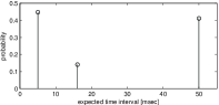
(a) Temporal coding ($\kappa=3$).

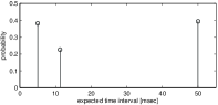
(b) Rate coding ($\kappa=3)$.

Figure 4: Capacity achieving distributions for temporal and rate coding. For both coding types, the optimal input distribution is discrete, with a finite number of probability mass points.

Rate Coding

In rate coding, a time window is set and the number of spikes in this interval is counted. Let us denote the interval and the rate as $\Delta$ and $R$, respectively, and define the distribution of $R$ as $p(r|\theta;\kappa,\Delta)$. The form of the distribution of $R$ is shown in Ikeda and Manton (2009). For $\pi\in\mathcal{P}$, let us define the following marginal distribution

$$p(r;\pi,\kappa,\Delta)=E_{\pi(\Theta)}[p(r|\theta;\kappa,\Delta)].$$

The mutual information of $R$ and $\theta$ is defined as

$$I(\Theta;R)=E_{\pi(\Theta)}\biggl{[}E_{p(R|\theta;\kappa,\Delta)}\Bigl{[}\log\frac{p(r|\theta;\kappa,\Delta)}{p(r;\pi,\kappa,\Delta)}\Bigr{]}\biggr{]}.$$

Hence, the capacity per channel use or equivalently per $\Delta$ is defined as

$$C_{R}=\sup_{\pi\in\mathcal{P}}I(\Theta;R).$$

This optimisation problem cannot be solved analytically either, but the capacity $C_{R}$ has been proven to be achievable by a discrete distribution with a finite number of mass points (Ikeda and Manton, 2009). Figure 4b shows the capacity achieving distribution for $\kappa=3$. The channel capacity $C_{R}$is 44.95 bits per second (See Ikeda and Manton (2009) for further results).

4.3 Tuning Curves

The definition of channel capacity requires a maximisation over all possible input probability distributions. This definition arose in an engineering context, where a system designer is assumed to have control over the inputs to the channel, but not the channel itself. A different optimisation problem results if the input to the channel is assumed to be fixed, but some control over the channel is possible. This idea is particularly relevant for studies of biological sensory transduction. In this context, an external stimulus that cannot be controlled by the sensing organism must be transduced and encoded into action potentials for communication to the brain. This stimulus can be thought of as an input to a communication channel.

Given internal noise in the transduction mechanisms, the encoded stimulus received by the brain is also noisy. Since we introduced mutual information in the context of the channel coding theorem and digital data, and here our channel input is a sensory stimulus, mutual information may not seem relevant. However there are other reasons why it can be useful to ensure mutual information is as large as possible (Berger, 2003; Johnson and Goodman, 2008) and we therefore are interested in how the channel might be altered to maximise mutual information.

But what can be optimised when the stimulus cannot be controlled? The only other variable that can alter the mutual information is the conditional distribution of the channel output given its input. In the biological context this is the distribution of a neural response for a given stimulus. Optimising this distribution means seeking to find the communication channel that it best suited to a fixed stimulus distribution. Without some constraints on the form of the conditional distribution, this would not be a meaningful task. One such constraint is to consider a fixed form for the conditional distribution that has some parameters that can be optimised. Clearly the optimal parameter set may change for different input distributions.

One reason for considering such an optimisation might be to assess whether neuronal mechanisms exist for adaptively altering the conditional distribution to match non-stationary stimuli. Another equally intriguing reason is the idea that evolution might have enabled neural systems to change parameters over eons with the end result that those parameters are information theoretically optimal. In this scenario, the underlying fixed form of the probability distribution must be what it is due to unavoidable constraints, or perhaps governed by criteria that are not information theoretic, e.g. energy considerations (Laughlin et al., 1998; Sarpeshkar, 1998; Levy and Baxter, 2002; Laughlin and Sejnowski, 2003; Berger and Levy, 2010).

There are several potentially important sets of parameters that might be chosen. However, in other contexts there has been much interest in determining the optimal form of neuronal tuning curves, and this is our sole focus here. Experimentally produced tuning curves are plots of the mean response of a neural system, as a function of a stimulus parameter (Dayan and Abbott, 2001; Lansky et al., 2008; McDonnell and Stocks, 2008). Classic examples of a stimulus parameter include the angle of a moving bar of light relative to the receptive field of visual cells, or the sound pressure level of a single frequency (pure tone) sound played by a speaker. In these examples the average response as a function of the stimulus defines the tuning curve. The former kind of tuning curve typically has a bell-shape, meaning that there is a stimulus that produces a maximal response, while more than one stimulus can produce the same lesser response. The latter kind has a sigmoidal shape, meaning that the mean firing rate monotonically increases with stimulus, and here we focus only on this case.

We therefore wish to find the sigmoidal tuning curve that maximises mutual information, for a given fixed form of a conditional distribution. While this is generally a difficult optimisation problem, a simple solution exists for channels where the capacity achieving input distribution is discrete, like those considered in this paper. In fact, the mutual information maximising tuning curve can be derived for an arbitrary stimulus distribution, if the capacity achieving input distribution has been calculated first. The reason for this is explained in the following.

We consider the same noisy channel as Section 4.2, that is the ISIs are governed by a gamma distribution. We now make a slight generalisation to the setup of Sections 4.1 and 4.2 and consider the expectation of the ISIs to be governed by a random variable $X$ with a known distribution, such that $\Theta$ is an arbitrary function of $X$.

We therefore write $\Theta=f(X)$. For the gamma ISI channel, the tuning curve is defined as the conditional expectation of the response variable (either $T$ or $R$) given a specified outcome of $X$. For timing coding or rate coding respectively, we write these expectations as

$$E_{p(T|x;\kappa)}[t]=\kappa f(x)$$

and

$$E_{p(R|x;\kappa,\Delta)}[r]=\frac{\Delta}{\kappa f(x)}.$$

Since $\Theta=f(X)$, when the capacity achieving distribution for $\Theta$ is discrete with say $M$ states, the tuning curve will also consist of $M$ unique values. Lets call these $\mu_{1}$,..,$\mu_{M}$. While this discontinuous tuning curve achieves the largest possible mutual information for the channel, it is not unique; other tuning curves are equally good. Suppose $X$ is a continuous random variable, and that the tuning curve maps large intervals of $X$ to the same $M$ values $\mu_{1}$, $\ldots$, $\mu_{M}$. This tuning curve provides the same $M$ possibilities for the conditional expected ISI. In order for it to provide the same mutual information achieved by the original discrete capacity achieving distribution, it is necessary that the probability with which each $\mu_{m}$ occurs is the same in both cases. It has been proven for a special case of the gamma distribution and rate coding that this can be achieved by appropriate choice for the ranges of $X$ that are mapped to each $\mu_{m}$. The resulting optimal discrete tuning curve is then dependent only on the probability density function of $X$ (Nikitin et al., 2009).

Consequently, the capacity achieving input distributions derived in Section 4.3 can be converted to an optimal tuning curve for any choice of the stimulus distribution. An example of the capacity achieving tuning curve is shown in Figure 5, for the special case of $\kappa=1$, which means the channel is equivalent to a Poisson neuron (Nikitin et al., 2009). The maximum rate is restricted to 30 spikes per input sample.

Although such a result holds exactly only for discrete input distributions, similar derivations of information theoretically optimal continuous tuning curves have been made, which hold only in the low noise limit (McDonnell and Stocks, 2008). See Kostal and Lansky (2010); Kostal (2010) for related work in the high noise limit.

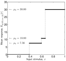
Figure 5: Channel capacity achieving tuning curve for a Poisson rate-coding neuron ($\kappa=1$), and an input $x\in[0,1]$, with a maximum spike-rate of 30 spikes per input sample—see Nikitin et al. (2009) for further examples.

4.4 Discussion and Interpretation

We have shown our results on neuron channel capacity from two very different viewpoints. Interestingly, both show that the capacity is achieved by a discrete distribution. The numerically computed capacities are similar to the range indicated by some biologically measured results of sensory neurons (Borst and Theunissen, 1999). The channel capacity depends on various factors, and we consider some of them below.

4.5 Input and Output

We first discuss the input and output of the neuron channel in this subsection.

Let us start with the input. Although each neuron receives information from many neurons, we have only considered a single input $\theta$. This may seem too simple. We assumed that the single input $\theta$ summarises all the inputs to the neuron. Moreover, $\theta$ has been assumed to be memoryless and can have any distribution within the support. Considering the biological system, this is far from realistic. The net input of a neuron may not change quickly, that is, it has memory. Moreover, a neuron’s input is a collection of many neurons’ noisy outputs, therefore, it may follow a particular probability distribution. This implies that we have computed capacity under less restrictive assumptions, and the biologically achievable rate should be smaller than the capacity obtained in the numerical studies. A better understanding of the constraints on the input of a neuron would lead to a more accurate calculation of neuronal channel capacity.

Next, we discuss the output of a neuron from two viewpoints, decoding and demodulation.

In order to achieve channel capacity, the receiver must act as an optimal decoder, meaning that when $\tilde{X}$ is observed, the receiver must compute the posterior distribution of the input $X$ as $p(x|\tilde{x}).$ When $x$ takes discrete values $x_{1},\cdots,x_{L}$, it becomes $p(x_{i}|\tilde{x}).$ This is a real number for each $x_{i}$. In engineering, this type of decoding is called “soft decoding.” It seems unlikely that a neuronal mechanisms for carrying this out could exist, since a computation of the posterior distribution is necessary.

Another standard decoding technique is “hard decoding,” that is, only a single value of $x_{i}$ is chosen by the decoder. The optimal hard decoder chooses the one which maximises the posterior distribution, that is $\hat{x}_{i}=\mathrm{argmax}_{x_{i}}\,p(x_{i}|\tilde{x})$. It is possible to implement the optimal hard decoder without requiring the online computation of the posterior distribution. Indeed, the output space (the space where $\tilde{X}$ lies) can be divided into $L$ subspaces in advance, such that the $k$ th subspace contains all the points $\tilde{X}$ such that $x_{k}$ has the largest posterior probability given $\tilde{X}$. Therefore, the optimal hard decoder can be implemented by a “quantisation” or “thresholding” algorithm which simply checks to see which subspace $\tilde{X}$ lies in. Such an algorithm is often computationally simpler than computing first the posterior distribution.

When we consider information processing in the brain, a naive soft decoding seems difficult, at least for a single neuron. The hard decoding idea seems more natural. However, the information transmission rate of the best hard decoding is less than the best soft decoding. We should keep this point in mind. Further discussion is found in Ikeda and Manton (2009).

4.6 Discreteness

Under the assumptions made, we have shown that the capacity of a neuron is achieved by a discrete distribution with a finite number of probability mass points. In information theory, there are many other known types of channels for which channel capacity is achieved by a discrete distribution (Huang and Meyn, 2005). For example, although the capacity of an average power constrained additive Gaussian white noise channels is achieved by continuously valued Gaussian inputs, simply placing a constraint on the maximum amplitude of the channel means capacity is achieved by a discrete distribution (Smith, 1971).

Our results do not imply that “neuron signals are only using discrete levels.” On the contrary, we believe many neurons are using continuous levels. What is implied by our results is that those neurons cannot achieve the capacity and the actual rate of information transfer is therefore less than the capacity. Another implication is for the measurement of information capacity in neuroscience (Borst and Theunissen, 1999). Our result implies that only a small number of discrete ranges are sufficient for the input distribution to measure the information capacity of neural coding.

Information theory provides a way of quantifying whether discrete or continuously distributed signals are better for any given communication channel corrupted by random fluctuations. Many neuroscience studies quantify information using Shannon’s famous information capacity formula relating mutual information to signal-to-noise ratio. This formula is correct only for Gaussian additive noise channels (Cover and Thomas, 2006) — it relies on many assumptions, and if any are false it can significantly under- or over-estimate the true capacity (Berger and Gibson, 1998).

4.7 Further Points

Guessing the channel model is not straightforward. In particular, feedback is prevalent in many parts of the brain, which makes it much more difficult to relate changes in responses to inputs. One important example where it is known that the circuitry is solely feedforward is that of retinal cells (Jacobs et al., 2009). This example has been used to demonstrate that it is possible to rule out certain guesses of neural codes. Because this is based on optimal Bayesian decoding of a forced binary choice, it would be interesting to extend (Jacobs et al., 2009) beyond the binary limitation to that where the signals being coded may have many possibilities

What can we say about more complicated situations? For example, information processing of cortical neurons are not strictly feedforward and the information is shared by many neurons. If we assume every neuron is performing the same computation, and each neuron encodes and decodes information in the same way, it seems possible to extend our results. However, when different neurons encode information differently, the problem becomes very different. Understanding how the brain works in information theoretic terms is one of the grand challenges of this century.

5 Conclusions and Future Directions

Most information theory research to date has been predicated on an engineering viewpoint. The main thrust has been to design compression/decompression methods that compress source information to the limits given by its entropy (source coding), or to design error correction schemes and encoding/decoding methods that allow communication close to capacity.

On the other hand, the goal of neuroscience is instead to understand information processing in the brain.

This does not mean that information theory has no place in computational neuroscience. Information theory provides a way to measure information and to understand the limits of compression (namely, entropy) and communication (namely, mutual information and channel capacity).

A common “information theoretic” method in computational neuroscience is to obtain quantitative estimates of the mutual information between observed sets of data. Since various methods for the (difficult) problem of accurately estimating mutual information exist, the bigger difficulty is with using the result to say something about how the system works. Indeed, the actual goal of computational neuroscience is that of “system identification,” as engineers would call it.

If the brain uses spikes to transmit information (which on faster time-scales appears to be the case) then understanding the neural code — how the brain encodes information before sending it across the “channel” — is tantamount to understanding how the brain works. Indeed, if we would listen in to the messages as they are sent from one neuron to another, it would be relatively straightforward to determine what each neuron is doing.

Although system identification is not the forte of traditional information theory (Johnson, 2008), this is merely for historical reasons. With computational neuroscience as a main motivator, we predict that the next decade will see the expansion of information theory to include more powerful techniques for system identification, and possibly even an integration of control, computation and information theory into a unified framework.

Some recent information theoretic approaches in neuroscience that go beyond standard Shannon theory are summarized in the following list.

• While it is traditional in engineering to separately code an information source, and then channel code it for communication across a channel, it has been shown for some simple but instructive examples, that non-separation of these two aspects can achieve an optimal communication system with a vastly reduced complexity compared to separation (Gastpar et al., 2003). This fact is potentially important for neurobiological systems, where separation mechanisms seem implausible.

• Many studies have investigated whether the brain might have mechanisms for implementing Bayesian algorithms during decision making, prediction and pattern recognition (Rao and Ballard, 1999; S.Lee and Mumford, 2003; Knill and Pouget, 2004; George and Hawkins, 2009).

• The possibility of analog cortical error correcting codes has been proposed by Fiete et al. (2008).

• One limitation of Shannon theory is that its measures say nothing about directionality or causality. However, directed information theory has also been developed (Granger, 1969; Marko, 1973; Rissanen and Wax, 1987; Massey, 1990; Tatikonda and Mitter, 2009) and has recently been applied in neuroscience (Hesse et al., 2003; Eichler, 2006; Waddell et al., 2007; Amblard and Michel, 2011; Quinn et al., 2011).

• The relationship between control, information theory and thermodynamics has been discussed by Mitter and Newton (2005); Friston (2010); Mitter (2010).

Summarising our own modest contribution, we carefully came up with a simple neuron channel model based on biological evidence and computed the channel capacity of this model. Interestingly, it was proved that the channel capacity is achieved by a discrete distribution.

References

- Wiener (1948) Norbert Wiener. Cybernetics: or Control and Communication in the Animal and the Machine. The Massachusetts Institute of Technology, second edition, 1948.
- von Neumann (2000) John von Neumann. The Computer and the Brain. Yale University Press, second edition, 2000.
- Shannon and Weaver (1949) Claude E. Shannon and Warren Weaver. The Mathematical Theory of Communication. University of Illinois Press, 1949.
- Fischbach (1992) Gerald D. Fischbach. Mind and brain. Scientific American, 267(3):24–33, 1992.
- Sarpeshkar (1998) Rahul Sarpeshkar. Analog versus digital: Extrapolating from electronics to neurobiology. Neural Computation, 10(7):1601–1638, 1998.
- Berger (2003) T. Berger. Living information theory: The 2002 Shannon lecture. IEEE Information Theory Society Newsletter, 53:1,6–19, 2003.
- Burdet et al. (2001) Etienne Burdet, Rieko Osu, David W. Franklin, Theodore E. Milner, and Mitsuo Kawato. The central nervous system stabilizes unstable dynamics by learning optimal impedance. Nature, 414:446–449, November 2001.
- Marko (1967) H. Marko. Information theory and cybernetics. Spectrum, IEEE, 4(11):75–83, nov. 1967.
- Todorov and Jordan (2002) Emanuel Todorov and Michael I. Jordan. Optimal feedback control as a theory of motor coordination. Nat Neurosci, 5(11):1226–1235, 11 2002.
- Burdet et al. (2006) E. Burdet, K. Tee, I. Mareels, T. Milner, C. Chew, D. Franklin, R. Osu, and M. Kawato. Stability and motor adaptation in human arm movements. Biological Cybernetics, 94:20–32, 2006.
- Franklin et al. (2008) David W. Franklin, Etienne Burdet, Keng Peng Tee, Rieko Osu, Chee-Meng Chew, Theodore E. Milner, and Mitsuo Kawato. CNS Learns Stable, Accurate, and Efficient Movements Using a Simple Algorithm. J. Neurosci., 28(44):11165–11173, 2008.
- Varshney et al. (2006) L. R. Varshney, P. J. Sjöström, and D. B. Chklovskii. Optimal information storage in noisy synapses under resource constraints. Neuron, 52:409–423, 2006.
- Buzsáki (2006) G. Buzsáki. Rhythms of the Brain. Oxford University Press, Oxford, UK, 2006.
- Cohen (2004) J. E. Cohen. Mathematics is biology’s next microscope, only better; biology is mathematics’ next physics, only better. PLoS Biology, 2:e439, 2004.
- Landauer (1986) Thomas K. Landauer. How much do people remember? some estimates of the quantity of learned information in long-term memory. Cognitive Science, 10:477–493, 1986.
- Shannon (1948) Claude E. Shannon. A mathematical theory of communication. The Bell System Technical Journal, 27:379–423 and 623–656, July and October 1948.
- Johnson (2008) D. H. Johnson. Information theory and neuroscience: Why is the intersection so small? In Proc. Information Theory Workshop, 5-9 May 2008, pages 104–108, 2008.
- Berger and Gibson (1998) T. Berger and J. D. Gibson. Lossy source coding. IEEE Transactions on Information Theory, 44:2693–2723, 1998.
- Borst and Theunissen (1999) A. Borst and F. E. Theunissen. Information theory and neural coding. Nature Neuroscience, 2:947–957, 1999.
- Panzeri et al. (2007) Stefano Panzeri, Riccardo Senatore, Marcelo A. Montemurro, and Rasmus S. Petersen. Correcting for the sampling bias problem in spike train information measures. J. Neurophysiol, 98:1064–1072, 2007.
- Vu et al. (2009) Vincent Q. Vu, Bin Yu, and Robert E. Kass. Information in the nonstationary case. Neural Computation, 21:688–703, March 2009.
- Rieke et al. (1997) F. Rieke, D. Warland, R. de Ruyter van Steveninck, and W. Bialek. Spikes: Exploring the Neural Code. MIT Press, Cambridge, MA., 1997.
- Poggio (1964) G. Poggio. Time series analysis of impulse sequences of thalamic somatic sensory neurons. Journal of Neurophysiology, 27:517–545, 1964.
- Mainen and Sejnowski (1995) Zachary F. Mainen and Terrence J. Sejnowski. Reliability of spike timing in neocortical neurons. Science, 268:1503–1506, June 1995.
- MacKay and McCulloch (1952) Donald M. MacKay and Warren S. McCulloch. The limiting information capacity of a neuronal link. Bull. Math. Biophys., 14:127–135, 1952.
- Stein (1967) R. B. Stein. The information capacity of nerve cells using a frequency code. Biophysical Journal, 7:797–826, 1967.
- Lansky et al. (2004) P. Lansky, R. Rodriguez, and L. Sacerdote. Mean instantaneous firing frequency is always higher than the firing rate. Neural Computation, 16:477–489, 2004.
- Johnson (2010) D. H. Johnson. Information theory and neural information processing. IEEE Transactions on Information Theory, 56:653–666, 2010.
- Suksompong and Berger (2010) P. Suksompong and T. Berger. Capacity analysis for integrate-and-fire neurons with descending action potential thresholds. IEEE Transactions on Information Theory, 56:838–851, 2010.
- Ikeda and Manton (2009) S. Ikeda and J. H. Manton. Capacity of a single spiking neuron channel. Neural Computation, 21:1714–1748, 2009.
- Johnson and Goodman (2008) D. H. Johnson and I. N. Goodman. Inferring the capacity of the vector Poisson channel with a Bernoulli model. Network: Computation in Neural Systems, 19:13–33, 2008.
- Laughlin et al. (1998) S. B. Laughlin, R. R. de Ruyter van Steveninck, and J. C. Anderson. The metabolic cost of neural information. Nature Neuroscience, 1(1):36–41, 1998.
- Levy and Baxter (2002) W. B. Levy and R. A. Baxter. Energy-efficient neuronal computation via quantal synaptic failures. The Journal of Neuroscience, 22:4746–4755, 2002.
- Laughlin and Sejnowski (2003) S. B. Laughlin and T. J. Sejnowski. Communication in neuronal networks. Science, 301:1870–1874, 2003.
- Berger and Levy (2010) T. Berger and W. B. Levy. A mathematical theory of energy efficient neural computation and communication. IEEE Transactions on Information Theory, 56:852–874, 2010.
- Dayan and Abbott (2001) P. Dayan and L. F. Abbott. Theoretical Neuroscience: Computational and Mathematical Modeling of Neural Systems. The MIT Press, 2001.
- Lansky et al. (2008) P. Lansky, O. Pokora, and J. P. Rospars. Classification of stimuli based on stimulus-response curves and their variability. Brain Research, 1225:57–66, 2008.
- McDonnell and Stocks (2008) M. D. McDonnell and N. G. Stocks. Maximally informative stimuli and tuning curves for sigmoidal rate-coding neurons and populations. Physical Review Letters, 101:058103, 2008.
- Nikitin et al. (2009) A. P. Nikitin, N. G. Stocks, R. P. Morse, and M. D. McDonnell. Neural population coding is optimized by discrete tuning curves. Physical Review Letters, 103:138101, 2009.
- Kostal and Lansky (2010) L. Kostal and P. Lansky. Information transfer for small-amplitude signals. Physical Review E, 81:050901, 2010.
- Kostal (2010) L. Kostal. Information capacity in the weak-signal approximation. Physical Review E, 82:026115, 2010.
- Huang and Meyn (2005) J. Huang and S. P. Meyn. Characterization and computation of optimal distributions for channel coding. IEEE Transactions on Information Theory, 51:2336–2351, 2005.
- Smith (1971) J. Smith. The information capacity of amplitude- and variance-constrained scalar Gaussian channels. Information and Control, 18:203–219, 1971.
- Cover and Thomas (2006) T. M. Cover and J. A. Thomas. Elements of Information Theory. Wiley, New York, second edition, 2006.
- Jacobs et al. (2009) A. L. Jacobs, G. Fridman, R. M. Douglas, N. M. Alam, P. E. Latham, G. T. Prusky, and S. Nirenberg. Ruling out and ruling in neural codes. Proceedings of the National Academy of Sciences of the USA, Early Edition:1–6, 2009.
- Gastpar et al. (2003) M. Gastpar, B. Rimoldi, and M. Vetterli. To code, or not to code: Lossy source–channel communication revisited. IEEE Transactions on Information Theory, 49:1147–1158, 2003.
- Rao and Ballard (1999) R. P. N. Rao and D. H. Ballard. Predictive coding in the visual cortex: a functional interpretation of some extra-classical receptive-field effects. Nature Neuroscience, 2:79–87, 1999.
- S.Lee and Mumford (2003) T. S.Lee and D. Mumford. Hierarchical Bayesian inference in the visual cortex. JOSA A, 20:1434–1448, 2003.
- Knill and Pouget (2004) D. C. Knill and A. Pouget. The Bayesian brain: the role of uncertainty in neural coding and computation. Trends in Neurosciences, 27:712–719, 2004.
- George and Hawkins (2009) D. George and J. Hawkins. Towards a mathematical theory of cortical micro-circuits. PLoS Computational Biology, 5:e1000532, 2009.
- Fiete et al. (2008) I. R. Fiete, Y. Burak, and T. Brookings. What grid cells convey about rat location. Journal of Neuroscience, 28:6858, 2008.
- Granger (1969) C. W. J. Granger. Investigating causal relations by econometric models and cross-spectral methods. Econometrica, 37:424–438, 1969.
- Marko (1973) H. Marko. The bidirectional communication theory–a generalization of information theory. IEEE Transactions on Communications, 21:1345–1351, 1973.
- Rissanen and Wax (1987) J. Rissanen and M. Wax. Measures of mutual and causal dependence between two time series. IEEE Transactions on Information Theory, 33:598–601, 1987.
- Massey (1990) J. Massey. Causality, feedback and directed information. In Proc. 1990 Intl. Symp. on Info. Th. and its Applications, pages 27–30. Citeseer, 1990.
- Tatikonda and Mitter (2009) S. Tatikonda and S. Mitter. The capacity of channels with feedback. IEEE Transactions on Information Theory, 55:323–349, 2009.
- Hesse et al. (2003) W. Hesse, E. Mõller, M. Arnold, and B. Schack. The use of time-variant EEG Granger causality for inspecting directed interdependencies of neural assemblies. Journal of Neuroscience Methods, 124:27–44, 2003.
- Eichler (2006) M. Eichler. On the evaluation of information flow in multivariate systems by the directed transfer function. Biological Cybernetics, 94:469–482, 2006.
- Waddell et al. (2007) J. Waddell, R. Dzakpasu, V. Booth, B. Riley, J. Reasor, G. Poe, and M. Zochowski. Causal entropies–A measure for determining changes in the temporal organization of neural systems. Journal of Neuroscience Methods, 162:320–332, 2007.
- Amblard and Michel (2011) P.-O. Amblard and O. J. J. Michel. On directed information theory and Granger causality graphs. Journal of Computational Neuroscience, 30:7–16, 2011.
- Quinn et al. (2011) C. J. Quinn, T. P. Coleman, N. Kiyavash, and N. G. Hatsopoulos. Estimating the directed information to infer causal relationships in ensemble neural spike train recordings. Journal of Computational Neuroscience, 30:17–44, 2011.
- Mitter and Newton (2005) S. K. Mitter and N. J. Newton. Information and entropy flow in the Kalman–Bucy filter. Journal of Statistical Physics, 118:145–176, 2005.
- Friston (2010) K. Friston. The free-energy principle: a unified brain theory? Nature Reviews Neuroscience, 11:127–138, 2010.
- Mitter (2010) S. K. Mitter. Towards a unified view of inference, communication and control. In 2010 International Conference on Signal Processing and Communications (SPCOM), pages 1–2. IEEE, 2010.