Fractal Structure of Equipotential Curves on a Continuum Percolation Model

Abstract

We numerically investigate the electric potential distribution over a two-dimensional continuum percolation model between the electrodes. The model consists of overlapped conductive particles on the background with an infinitesimal conductivity. Using the finite difference method, we solve the generalized Laplace equation and show that in the potential distribution, there appear the quasi-equipotential clusters which approximately and locally have the same values like steps and stairs. Since the quasi-equipotential clusters have the fractal structure, we compute the fractal dimension of equipotential curves and its dependence on the volume fraction over $[0,1]$. The fractal dimension in [1.00, 1.246] has a peak at the percolation threshold $p_{c}$.

1 Introduction

In the series of articles [1, 2], we have studied the electric conductivity of a percolation model using the finite difference method (FDM) [3]. The purpose of these studies is to reveal the electric properties over the continuum percolation model (CPM). As we explored three dimensional shape effects on the conductivity on CPMs in the previous articles [1, 2], in this article we investigate the fractal properties of the solutions of the two dimensional generalized Laplace equation,

$$\nabla\cdot\sigma\nabla\phi=0,$$ (1)

for the conductivity distribution $\sigma(x,y)$ of CPM. Recently materials consisting of the conductive particles in a base material with extremely high resistance are studied [4, 5, 6]. We handle the binary local conductivities $\sigma(x,y)$ of the binary materials in CPM, i.e., conductive particles in the background with an infinitesimal conductivity. The infinitesimal conductivity, i.e., the extremely high resistance, avoids indeterminacy of the solutions of (1) all over there, because approaching to zero differs from the zero itself.

Two dimensional CPMs of the overlapped circles were studied well in Refs.[7] and [8] and references therein. In this article, we also deal only with CPM whose particles are overlapped circles with the same radius.

As the solution of the generalized Laplace equation (1) provides the electric potential distribution, we show that there exist quasi equipotential clusters, in which the potential behaves like steps and stairs approximately. There are many pieces whose potentials are approximately flat because their electric connections are very small and thus the resistances are so high at the boundaries whereas the inner resistance of the pieces or the composite particles is very small.

The existence of the quasi-equipotential clusters means the anomalous behaviors of the equipotential curves. Though the relation between the percolation cluster and fractal structure has been studied [8], in this article, we provide the result how the fractal dimension of the equipotential curves behaves depending on the volume fraction $p\in[0,1]$. Under the percolation threshold $p_{c}$, our computation can read the computation of dielectric behavior on a random configuration of metal particles in the dielectric matter, which was reported in Refs. [9] and [10] if we interpret the conductivity as the dielectric constant.

Further recently, some classes of statistical models including several two dimensional percolation models and the self-avoiding random walk have investigated in the framework of Schramm-Loewner evaluation (SLE) and conformal field theory [11, 12, 13, 14, 15]. Using their conformal properties, it is proved rigorously that some of the universal quantities such as the critical exponent and the fractal dimension are expressed by rational numbers such as 5/4 and 4/3. Since by taking a certain limit, the potential $\phi$ in (1) can show the conformal property, it is expected that our numerical computational results should be also interpreted in their framework in future. We give some comments in Sec.3.3.

Contents in this article are as follows. Sec.2 gives our computational method; Sec. 2.1 is on the geometrical setting in CPMs and Sec. 2.2 gives the computational method of the conductivity over CPMs using FDM, which is basically the same as that in the previous article [1]. Sec. 3 shows our computational results of the solutions of (1) in CPMs, and we discuss our results from physical viewpoints there.

2 Computational method

In this section, we explain our computational method of CPM. Though we deal only with two dimensional case, its essential is the same as the three dimensional case using FDM [3] whose detail is in the previous article [1].

2.1 Geometrical setting

We set particles parametrized by their positions $(x,y)$ into a box-region ${\mathcal{B}}:=[0,x_{0}]\times[0,y_{0}]$ at random and get a configuration ${\mathfrak{R}}_{n}$ as one of CPMs. In this article, we set $x_{0}=y_{0}=L_{a}$, and handle three boxes ${\mathcal{B}}_{a}$ $(a=1,2,3)$ with different size, $L_{1}=40.96$, $L_{2}=81.92$, and $L_{3}=163.84$. The particle corresponds to a stuffed circle with the same radius $\rho=1$, $B_{x_{i},y_{i}}:=\{(x,y)\in{\mathcal{B}}\ |\ |(x,y)-(x_{i},y_{i})|\leq\rho\}$. The configuration ${\mathfrak{R}}_{n}$ is given by ${\mathfrak{R}}_{n}:=\bigcup_{i=1}^{n}B_{x_{i},y_{i}}$, where each center $(x_{i},y_{i})$ is given at uniform random in ${\mathcal{B}}$. We allow their overlapping.

By monitoring the total volume fraction which is a function of ${\mathfrak{R}}_{n}$ and is denoted by ${\rm{vol}}({\mathfrak{R}}_{n})$, we continue to put the particles as long as ${\rm{vol}}({\mathfrak{R}}_{n})\leq p$ for the given volume fraction $p$. We find the step $n(p)$ such that ${\rm{vol}}({\mathfrak{R}}_{n(p)-1})\leq p$ and ${\rm{vol}}({\mathfrak{R}}_{n(p)})>p$. The difference between ${\rm{vol}}({\mathfrak{R}}_{n(p)-1})$ and ${\rm{vol}}({\mathfrak{R}}_{n(p)})$ is at most $1.87\times 10^{-3}$ for ${\mathcal{B}}_{1}$, $4.68\times 10^{-4}$ for ${\mathcal{B}}_{2}$, and $1.17\times 10^{-4}$ for ${\mathcal{B}}_{3}$, we regard ${\rm{vol}}({\mathfrak{R}}_{n(p)})$ as each $p$ hereafter under this accuracy.

Since we use the pseudo-randomness to simulate the random configuration ${\mathfrak{R}}_{n(p)}$ for given $p$, the configuration ${\mathfrak{R}}_{n(p)}$ depends upon the seed $i_{s}$ of the pseudo-random which we choose and thus let it be denoted by ${\mathfrak{R}}_{p,i_{s}}$. For the same seed $i_{s}$ of the pseudo-random, a configuration ${\mathfrak{R}}_{p,i_{s}}$ of a volume fraction $p$ naturally contains a configuration ${\mathfrak{R}}_{p^{\prime},i_{s}}$ of $p^{\prime}<p$ due to our algorithm. Hence the elements in the set of the configurations $\{{\mathfrak{R}}_{p,i_{s}}\ |\ p\in[0,1]\}$ with the same seed $i_{s}$ are relevant. Fig.1 illustrates the configurations of the seed $i_{s}=1$ for several $p$.

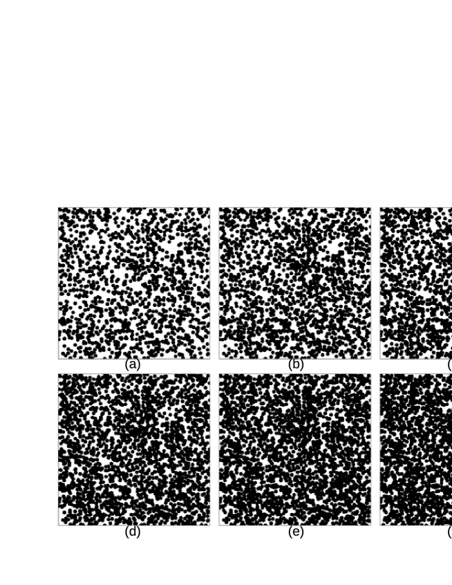
Figure 1: The configurations of the seed $i_{s}=1$ with the volume fractions 0.5, 0.6, 0.65, 0.7, 0.75, 0.8 for (a), (b), (c), (d), (e), (f) respectively.

2.2 Computation of the potentials in CPM

To apply FDM to the generalized Laplace equation in CPM, we use three lattices, $1024\times 1024$, $2048\times 2048$, and $4096\times 4096$, to represent the ${\mathcal{B}}_{1}$, ${\mathcal{B}}_{2}$ and ${\mathcal{B}}_{3}$ respectively. The radius of the particle $\rho=1$ corresponds to $25$ meshes.

Further we set the binary local conductivity $\sigma(x,y)$ which consists of the conductive particles with the conductivity density $\sigma_{\rm{mat}}=1$, and the background with infinitesimal conductivity $\sigma_{{\rm{inf}}}=10^{-4}$.

In order to compute the potential distribution $\phi(x,y)$, we set $\phi=1$ and $\phi=0$ on the upper and the lower segments respectively as the boundary condition corresponding to the electrodes. As the side boundary condition, we use the natural boundary for each $y$-boundary so that current normal to each boundary vanish.

Following our algorithm of FDM as mentioned in detail in Ref.[1], we numerically solve the generalized Laplace equations (1) for the conductivity distribution $\sigma(x,y)$ of each ${\mathfrak{R}}_{p,i_{s}}$.

Then we obtain the total conductivity $\sigma_{\mathrm{total}}$ of the system after we integrate the current $\sigma\nabla\phi$ over the line parallel to the $x$-axis. Since $\sigma_{\mathrm{total}}$ is determined for each ${\mathfrak{R}}_{p,i_{s}}$, $\sigma_{\mathrm{total}}$ is a function of the volume fraction $p$ and the seed $i_{s}$ of the pseudo-random. We denote it by $\sigma_{\mathrm{total}}(p)$.

The dependence of the total conductivities on the volume fraction as a conductivity curve is given by

$$\sigma_{\mathrm{total}}(p)=\frac{(p-p_{c})^{t}}{(1-p_{c})^{t}}\theta(p-p_{c}),$$ (2)

where $p_{c}$ is the threshold, ${t}$ is the critical exponent, or merely called exponent, and $\theta$ is a Heaviside function, i.e., $\theta(x)=1$ if $x\geq 0$ and vanishes otherwise. (2) is represented by a difference between the holomorphic and anti-holomorphic functions in terms of the Sato hyperfunction theory [16]. As mentioned in Introduction, the conformal properties, which are given by the holomorphic and anti-holomorphic functions, in a two-dimensional percolation model are recently revealed [11, 17, 13], whereas the holomorphic function, in general, determines its global behavior from its local behavior because of the identity theorem in theory of the complex analysis. By considering these facts, we assume, in this article, that (2) is defined over $[0,1]$ rather than the restricted region around $p_{c}$. At least, from a viewpoint of numerical computations, the least square error method shows the good descriptions of the conductivity curves in terms of the equation (2) over $[0,1]$. Since the threshold $p_{c}$ and the exponent ${t}$ are determined by $\{{\mathfrak{R}}_{p,i_{s}}\ |\ p\in[0,1]\}$, they also depend on the seed $i_{s}$ of the pseudo-random.

3 The results and discussions

3.1 Conductivity curve

The ordinary computations of the conductivity over the percolation system are performed using the Y-$\Delta$ algorithm [18] by assuming that the conductivity of the background insulator vanishes [19]; (1) is not defined over there in the ordinary approaches.

In our computations using FDM, we handle the binary conductivity distribution $\sigma(x,y)$ due to the demands of the recent material science [4, 5, 6].

Even though we deal with the binary conductivity distribution with finitely different resistances, the conductivity curve is naturally obtained as in Fig.2.

(a)

(b)

Figure 2: Average of conductivity curves for ${\mathcal{B}}_{3}$; (a) for the linear total conductivity $\sigma_{\mathrm{total}}$ and (b) for its logarithm scale.

Fig.2(a) exhibits the linear scale behavior of average of the total conductivities in ${\mathcal{B}}_{3}$ whereas Fig.2(b) shows its logarithm property. Even though Fig.2(b) illustrates the property of the binary materials, the linear scale behavior of the total conductivity is described well by (2) because the ratio between the binary conductivities $\sigma_{\rm{mat}}$ and $\sigma_{\rm{inf}}$ is sufficiently large.

We computed six cases with different seeds $i_{s}$ of the pseudo-randomness for the three boxes, ${\mathcal{B}}_{1}$, ${\mathcal{B}}_{2}$, and ${\mathcal{B}}_{3}$ and determine the thresholds $p_{c}$ and the exponents ${t}$ using the least mean square method respectively.

(a)

(b)

Figure 3: Threshold and Exponent vs. Box-size: The filled circles show the individual values whereas the open circles correspond to their averages.

The obtained results are illustrated in Fig.3 and Table 1. Fig.3 shows the dependence of the threshold and the exponent on the size of boxes. The larger size of boxes is, the smaller the fluctuations of the threshold and the exponent are. These results are also listed in Table.1.

Table 1: The Size dependence of the threshold and the exponent:

	Threshold		Exponent
	Average	Max-Min	Average	Max-Min
${\mathcal{B}}_{1}$	0.669	0.097	1.229	0.690
${\mathcal{B}}_{2}$	0.664	0.059	1.297	0.312
${\mathcal{B}}_{3}$	0.661	0.032	1.312	0.190

The average of the percolation threshold is $0.66\pm 0.02$ for ${\mathcal{B}}_{3}$ which is equal to $0.6763475(6)$ reported in Ref. [20] within our accuracy and the exponent is given as $1.31\pm 0.10$ for ${\mathcal{B}}_{3}$ which approximately recovers the universal value $4/3$ of two-dimensional percolation [7] within this accuracy. Since the effect of the finite size of the analyzed region makes the threshold smaller, the difference comes from the finite size effect [1, 2]. The direct computation of the total conductivity using FDM provides the potential distribution as shown in Figs.4 and 5, but it is for a finite region. Though it is very important that we evaluate the magnitude of the fluctuation, it is difficult to remove these fluctuations in Fig.3 in our FDM computations. However in this article, we investigate the properties of the potential distributions and these fluctuations do not essentially affect our results which are shown as follows.

3.2 Potential distribution

By numerically solving (1), we obtain the potential distribution $\phi(x,y)$ for each volume fraction $p\in[0,1]$ and the seed $i_{s}$ of the pseudo-randomness as we display the results in Fig.4 for $i_{s}=1$. Fig.5 shows its equipotential curves for $\phi=0.1,0.2,\ldots,0.9$ of ${\mathcal{B}}_{3}$ with $i_{s}=1$. The interval of the equipotential curves $\delta\phi$ equals $0.1$.

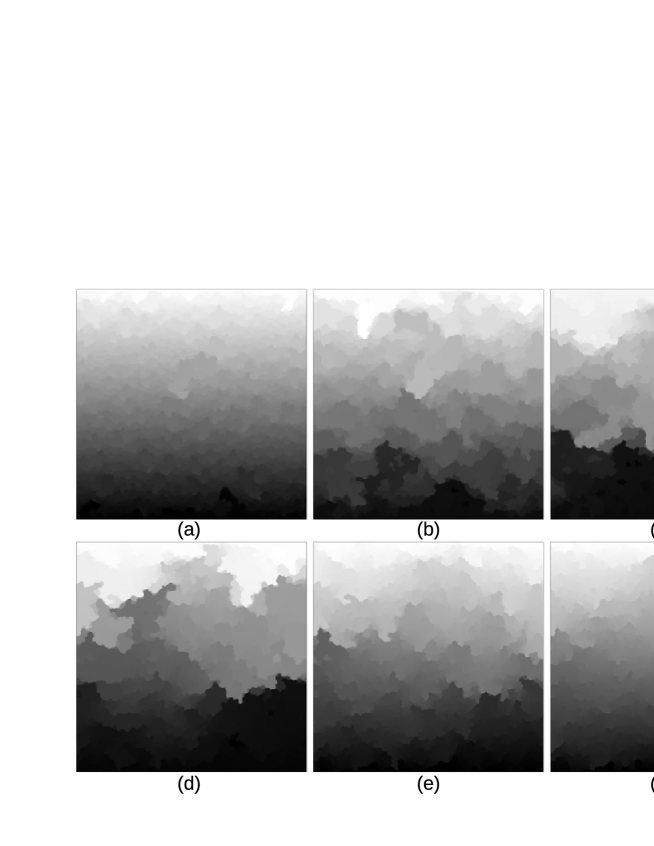
Figure 4: Potential distributions of the seed $i_{s}=1$ with the volume fractions 0.5, 0.6, 0.65, 0.7, 0.75, 0.8 for (a), (b), (c), (d), (e), (f) respectively. The black corresponds to $\phi=0$ whereas the white does to $\phi=1$. The graduated gray interpolates them. The quasi-potential clusters exist there.

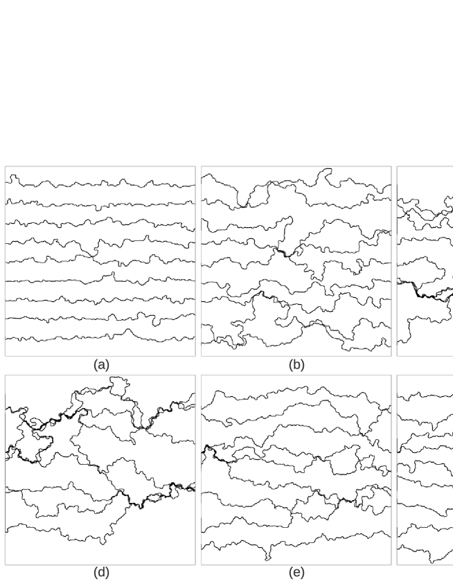
Figure 5: Equipotential curves of the potential distributions of the seed $i_{s}=1$ with the volume fractions 0.5, 0.6, 0.65, 0.7, 0.75, 0.8 for (a), (b), (c), (d), (e), (f) respectively. The curves correspond to the values $\phi=$ 0.1, 0.2, $\ldots$, 0.8, and 0.9. The interval of the curves $\delta\phi$ is $0.1$.

Fig.6 is parts of Fig.5 with the configurations of particles at $p=0.5<p_{c}$ and $p=0.8>p_{c}$. The contours basically run to avoid the conductive particles due to the difference of the local conductivity between $\sigma_{\rm{mat}}$ and $\sigma_{\rm{inf}}$. Especially in Fig.6(a) for the case $p=0.5$, the avoidance explicitly appears.

On the other hand, at $p=1$, the potential is simply described by $\phi(x,y)=y/y_{0}$ and the contours penetrate into the conductive particles. Thus even for $p=0.8$, the contours penetrate into the conductive particles. For the percolation clusters which are connected with both anode and cathode, the contours cross the clusters. On the other hand, around the approximately isolated percolation cluster which is not connected with electrodes approximately, the contours go through the (narrow) gaps among the conductive particles. Fig.6(b) contains the situations, in which the contours partially penetrate into the conductive particles and partially avoid the conductive particles. However due to the above considerations, these behaviors in Fig.6(b) can be naturally interpreted.

Further Fig.6 shows that the local equipotential curves depend upon the local configurations of these particles. For given resolution and local region, the sets of particles surrounding the region locally play the role of the electrodes and the direction of the locally averaged gradient, i.e., the local electric field, strongly depends upon the resolutions and upon the region which we average. For the locally averaged electric field within an appropriate scale $(L\gg a\gg 1)$, we may represent its local direction by O(2) value spin, and thus our model could be partially interpreted by XY-spin model with the external field coming from the electrodes. Since XY-model which is the O(2) valued spin system has the fractal structure [21], the randomness also brings the self-similar structure into our system.

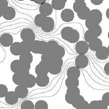
(a)

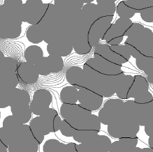
(b)

Figure 6: The equipotential curves with $\delta\phi=0.0125$, and the configurations of particles; (a) for $p=0.5$ and (b) for $p=0.8$.

Under the threshold $p_{c}$, this phenomenon is essentially the same as the one of dielectric properties related to the electric breakdown, which were studied by Gryure and Beale in Ref. [9] and recently by Stoyanov, Mc Carthy, Kollosche and Kofod in Ref. [10], though the authors handled the hard core model in which the overlapping is prohibited instead of our soft core CPMs. They studied the dielectric materials as background with infinite dielectric particles (metal particles), which are governed by the same generalized Laplace equation (1), though it is for the region of $p\in[0,p_{c}]$. Fig.6(a) corresponds to the Fig.1 in Ref. [9] if the conductivity reads the dielectric constant.

In our computational condition on the conductivity, we can determine the potential distributions over ${\mathcal{B}}$ for every volume fraction $p\in[0,1]$ due to the infinitesimal conductivity $\sigma_{\rm{inf}}$.

As objects in the percolation theory exhibit the fractal structures related to the percolation clusters [8], and to the breakdown [22, 23, 24, 25], the fractal dimension characterizes these properties. We also computed the fractal dimensions but especially ones of the equipotential curves in the following section.

3.3 Fractal dimension of equipotential curves

Fig.4 provides the 256 degree shading pictures, in which we find more complicate structures than those in Fig.5. Fig.4 illustrates that the generalized Laplace equation over a random configuration generates the self-similar structures. Fig.4 looks like pictures of the piled up mountains in distance using the monochrome water-painting. There are many pieces whose potentials are approximately flat, like leaves of the piled leaves. Mandelbrot stated in Ref. [26] that the fractal structures appear in many phenomena including geographical geometry and these behaviors exhibit universal properties, which are profound mathematically beyond a shabby resemblance. In fact, the recent studies in Refs. [11, 27, 12] show that the fractal structures are connected with wide fields in theoretical physics. In fact, these properties are interpreted that there exist quasi-equipotential clusters whose individual potential is approximately constant and behaves like steps and stairs. In other words, the electric connections among the pieces are very small and thus the resistance is so high at the connections whereas the inner resistance of the piece or the composite particles is quite small.

Let us consider the effect of the quasi-equipotential clusters on the equipotential curves in Figs.5 and 6, and the fractal dimensions of the equipotential curves. On the computation of the fractal dimensions, we used the box-counting method [26]. Since the curves in Fig.5 of the seed $i_{s}=1$ have the fractal structure, their fractal dimensions are not trivial.

(a)
(c)

(b)
(d)

Figure 7: The fractal dimension vs. volume fraction $p$ for six seeds: (a) for ${\mathcal{B}}_{2}$, (b) for ${\mathcal{B}}_{3}$, and (c) for their average behaviors with error bars. A dotted line and a solid line in (c) correspond to ${\mathcal{B}}_{2}$ and ${\mathcal{B}}_{3}$ respectively.

The dependence of the fractal dimensions $D(p)$ of the equipotential curves with the interval of the equipotential curves $\delta\phi=0.1$ on the volume fraction $p\in[0,1]$ for six different seeds $i_{s}$ is presented in Fig.7; Fig.7 (a) shows the behavior of ${\mathcal{B}}_{2}$, and (b) shows that of ${\mathcal{B}}_{3}$. Fig.7 (c) displays their average with error bars for their maximum and minimum values. Since the percolation threshold $p_{c}$ of ${\mathcal{B}}_{2}$ has larger fluctuation than one of ${\mathcal{B}}_{3}$, the fractal dimension $D(p)$ of ${\mathcal{B}}_{2}$ also has larger fluctuations than ones of ${\mathcal{B}}_{3}$. However both behaviors are essentially the same without depending on the size of the system.

Mandelbrot showed that the geographical curves like the coastlines sometimes show fractal behavior [26] and have the fractal dimensions 1.0$\sim$1.25. The equipotential curve is obviously a kind of self-avoiding curve which is given in the randomized configuration, though it is not clear whether the curve belongs to one of the universality classes, such as the self-avoiding random walk (SAW), the brownian frontier (BF), and the loop-erased self-avoiding walk (LESAW). It is known that these fractal dimensions of SAW, BF, and LESAW are 4/3, 4/3 and 5/4 respectively [15, 28, 14, 27]. Further it is also known that the front of percolation cluster has 4/3 dimension as results of numerical computations [7, 29].

Our fractal dimension $D(p)$ is in [1.00, 1.246] and has a peak at the threshold $p_{c}$. In other words, around $p_{c}$, the equipotential curves behave complicatedly and have the self-similar structures. On the other hand, for the $p=0$ and $p=1$ cases, the dimension must be equal to $1$. Due to larger fluctuation of the threshold, the curves in Fig.7 (a) looks rude. However these properties that the curve has the endings at $1$ and has a peak around $p_{c}$ are universal. Further the crudeness causes the values at the peaks larger than ones of Fig.7 (b). The larger the size of region is, the sharper the peak is, as shown in Fig.7 (c). It is difficult to find the peak value. Further the computation of (1) at the threshold $p_{c}$ basically needs a more rigorous numerical treatment than others because the singular behavior decrease the accuracy of the numerical computations. We carefully computed the value (using fine-tuned convergence parameters, and $\sigma_{{\rm{inf}}}=10^{-6}$) in ${\mathcal{B}}_{3}$ at $\overline{p_{c}}=0.661$, which is 1.255.

Further when we approach the threshold $p=p_{c}$ from below, the percolation cluster connecting with the electrode faces each other and they are nearly connected. Thus some of the equipotential curves overlap at the front of these percolation clusters as we partially find the overlaps with respect to the resolution in Fig 5. Similarly isolated percolation clusters also contribute the shape of the equipotential curves as the front of quasi equipotential clusters. In other words, the equipotential curves, at least partially, are expected to agree with the front of the percolation clusters whose the fractal dimension is known as 4/3. Thus it is expected that the fractal dimension $D(p)$ should have a peak at the percolation threshold $p=p_{c}$ whose value is larger than 1.246 and 1.255. Ziff conjectures that the dimension may be equal to $4/3$ at $p_{c}$ [30]. Since in the limit $\sigma_{\rm{inf}}\to+0$, the equation (1) over $p>p_{c}$ is reduced to the mixed Dirichlet-Neumann boundary problem of the Laplace equation with a random boundary, and $\phi$ is expressed by a real part of a holomorphic function, it is expected that our computational results might be also interpreted in the framework of SLE and conformal field theory.

References

- Matsutani et al. [2010] S. Matsutani, Y. Shimosako, Y. Wang, Numerical computations of conductivity in continuum percolation for overlapping spheroids, Int. J. Mod. Phys. C 21 (2010) 709–729.
- Matsutani et al. [2011] S. Matsutani, Y. Shimosako, Y. Wang, Numerical computaions of conductivity over agglomerated continuum percolation modes, arxiv.1107.2158, 2011.
- LeVeque [1955] R. J. LeVeque, Finite Difference Methods for Ordinary and Partial Differential Equations, SIAM, Philadelphia, 1955.
- Al-Saleh and Sundararaj [2008] M. H. Al-Saleh, U. Sundararaj, Nanostructured carbon black filled polypropylene/polystyrene blends containing styrene-butadiene-styrene copolymer: Influence of morphology on electrical resistivity, Eur. Polymer J. 44 (2008) 1931–1939.
- Tee et al. [2007] D. Tee, M. Mariatti, A. Azizan, C. See, K. Chong, Effect of silane-based coupling agent on the properties of silver nanoparticles filled epoxy composites, Comp. Sci. Tech. 67 (2007) 2584–2591.
- Konishi and Cakmak [2006] Y. Konishi, M. Cakmak, Nanoparticle induced network self-assembly in polymer carbon black composites, Polymer 47 (2006) 5371–5391.
- Isichenko [1992] M. B. Isichenko, Percolation, statistical topography, and transport in random media, Rev. Mod. Phys. (1992) 961–1043.
- Stauffer and Aharony [1991] D. Stauffer, A. Aharony, Introduction to percolation theory, revised second ed., CRC, Boca Raton, 1991.
- Gyure and Beale [1989] M. F. Gyure, P. D. Beale, Dielectric breakdown of a random array of conducting cylinders, Phys. Rev. B. 40 (1989) 9533–9540.
- Stoyanov et al. [2009] H. Stoyanov, D. M. Carthy, M. Kollosche, G. Kofod, Dielectric properties and electric breakdown strength of a subpercolative composite of carbon black in thermoplastic copolymer, Appl. Phys. Lett. 94 (2009) 232905.
- Cardy [2003] J. L. Cardy, Conformal invariance in percolation, self-avoiding walks, and related problems, Annales Henri Poincare (2003) 371–384.
- Lawler [2009] G. F. Lawler, Conformal invariance and statistical physics, Bull. Amer. Math. Soc. 46 (2009) 35–54.
- Smirnov [2001] S. Smirnov, Critical percolation in the plane: conformal invariance, cardy’s formula, scaling limits, C. R. Acad. Sci. Paris, Ser.I Math 333 (2001) 239–244.
- Lawler et al. [2001] G. F. Lawler, O. Schramm, W. Werner, The dimension of the planar brownian frontier is 4/3, Math. Res. Lett. 8 (2001) 401–411.
- Lawler et al. [2004] G. F. Lawler, O. Schramm, W. Werner, On the scaling limit of planar self-avoiding walk, in: M. Lapidus, M. van Frankenhuijsen (Eds.), Fractal Geometry and Applications: A Jubilee of Benoit Mandelbrot, Vol II, Amer. Math. Soc., New York, 2004, pp. 339–364.
- Imai [1992] I. Imai, Applied Sato hyperfunction theory, Kluwer, New York, 1992.
- Leveque [2007] R. J. Leveque, Finite Difference Methods for Ordinary and Partial Differential Equations: Steady-State and Time-Dependent Problems (Classics in Applied Mathematics), Soc. for Industrial & Applied, Natick, 2007.
- Johnson et al. [1997] D. E. Johnson, J. L. Hilburn, J. R. Johnson, P. D. Scott, Electric Circuit Analysis, third ed., John Wiley & Sons, New York, 1997.
- Garboczi et al. [1991] E. J. Garboczi, M. F. Thorpe, M. S. DeVries, A. R. Day, Universal conductivity curve for a plane containing random holes, Phys. Rev. A 43 (1991) 6473–6482.
- Quintanilla and Ziff [2007] J. A. Quintanilla, R. M. Ziff, Asymmetry in the percolation thresholds of fully penetrable disks with two different radii, Phys. Rev. E 76 (2007) 051115.
- Kroger [2000] H. Kroger, Fractal geometry in quantum mechanics, field theory and spin systems, Phys. Rep. 323 (2000) 81–181.
- Peruani et al. [2003] F. Peruani, G. Solovey, I. M. Irurzun, E. E. Mola, A. Marzocca, J. L. Vicente, Dielectric breakdown model for composite materials, Phys. Rev. E 67 (2003) 066121.
- Palevski and Deutscher [1984] A. Palevski, G. Deutscher, Conductivity measurement on percolation fractal, J. Phys. A 17 (1984) L895–L898.
- Fournier et al. [1997] J. Fournier, G. Boiteux, G. Seytre, Fractal analysis of the percolation network in epoxy-polypyrrole composites, Phys. Rev. B 56 (1997) 5207–5212.
- Lenormand [1989] R. Lenormand, Flow through porous media: Limits of fractal patterns, Proc. R. Soc. Lond. A 423 (1989) 159–168.
- Mandelbrot [1982] B. Mandelbrot, Fractal Geometry of Nature, Freeman, New York, 1982.
- Bauera and Bernard [2006] M. Bauera, D. Bernard, 2d growth processes: Sle and loewner chains, Phys. Rep. (2006) 115–221.
- Majumdar [1992] S. N. Majumdar, Exact fractal dimension of the loop-erased self-avoiding walk in two dimensions, Phys. Rev. Lett. 68 (1992) 2329–2331.
- Sapoval [2001] B. Sapoval, Universalites et fractales, Flammarion-Champs, Paris, 2001.
- Ziff [2011] R. M. Ziff, a private communication, 2011.