Aharonov-Bohm interference for a hole in a two-dimensional Ising antiferromagnet in a transverse magnetic field

Abstract

We show that a proper consideration of the contribution of Trugman loops leads to a fairly low effective mass for a hole moving in a square lattice Ising antiferromagnet, if the bare hopping and the exchange energy scales are comparable. This contradicts the general view that because of the absence of spin fluctuations, this effective mass must be extremely large. Moreover, in the presence of a transverse magnetic field, we show that the effective hopping integrals acquire an unusual dependence on the magnetic field, through Aharonov-Bohm interference, in addition to significant retardation effects. The effect of the Aharonov-Bohm interference on the cyclotron frequency (for small magnetic fields) and the Hofstadter butterfly (for large magnetic fields) is analyzed.

I Introduction

Ever since the discovery of high-temperature superconductivity in cuprates,Bednorz and Müller (1986) understanding the motion of a hole in an otherwise half-filled CuO₂ layer has been a major challenge in condensed matter physics.Berciu (2009) If, as most customary, one models this system with a one-band Hubbard model,Hubbard (1963); *Ka63 then in the limit of a large on-site repulsion $U$ the half-filled case maps onto an antiferromagnetic (AFM) Heisenberg Hamiltonian with spin-exchange coupling $J=4t^{2}/U$, where $t$ is the nearest-neighbor (NN) hopping.Gros et al. (1987) In this limit, then, the problem reduces to understanding the motion of a hole in a two-dimensional (2D) AFM background.Trugman (1988); Kane et al. (1989); Martinez and Horsch (1991)

A major reason for the difficulty in dealing with this question is that despite being long-range ordered at $T=0$, the undoped AFM background has a very complicated wavefunction due to spin fluctuations, which make it very unlike the semi-classical Néel state. A simple but more realistic description that could be used for analytical purposes is missing; as a result, progress has been made primarily through numerical simulations.Dagotto et al. (1990); *FWRB91; *Da94; Lee et al. (2006); *Le08

Here, we present an essentially exact numerical solution, and an approximate but quite accurate analytical approach, for the much simpler issue of a hole moving in an Ising AFM background,Shraiman and Sigga (1988); *EBS90 whose undoped wavefunction is the Néel state. The solutions have a variational interpretation, and are shown to be accurate for a wide range of parameters, of up to $t/J\approx 3$.

The generally accepted view, which probably explains why this problem has not been solved so far (to the best of our knowledge), is that a hole cannot really move in an Ising AFM, since as it hops away from its initial location it re-shuffles the spins at the sites it visits, creating a string of “defects” (misaligned spins). In dimensions higher than one, the energy cost of this string increases roughly linearly with its length, and as a result the hole is forced to stay in the vicinity of its original position, i.e. its effective mass is infinite.Brinkman and Rice (1970) In this view, spin fluctuations which effectively remove (or “heal”) pieces of this string of defects are needed to free the hole and allow it to acquire a finite effective mass. Of course, such spin fluctuations are absent in an Ising AFM.

That the hole is not truly localized even in an Ising AFM has been known ever since Trugman pointed outTrugman (1988) that by going twice around a closed loop, the hole can actually acquire a finite effective mass. We will return to this in more detail below, but the main idea is that while the first circuit along the closed loop creates the usual chain of defects, the second reshuffle of the spins during the second circuit removes all these defects, but also ends with the hole at a different location than the original site. By repeating such processes, the hole can therefore move anywhere on its original sublattice.

Even though Trugman started from a Néel background and identified this mechanism for generating a finite quasiparticle mass in the absence of spin fluctuations, he included spin-fluctuations in his calculation by considering the full Heisenberg AFM Hamiltonian when determine the effective mass of the hole.Trugman (1988) The issue of the hole mass in a purely Ising AFM thus remained unanswered.

Here we carry out this calculation, and show that the hole is fairly mobile if $t\sim J$. Moreover, if a transverse magnetic field is turned on, due to Aharonov-Bohm interference of the Peierls phases associated with these closed loops, the effective hoppings acquire a magnetic field dependence over and above the usual Peierls phases, with interesting consequences. Our results reveal that even this seemingly simple problem is actually very interesting and leads to rather non-trivial results.

The paper is organized as follows. In Sec. II, we specify the model and our notation. In Sec. III, we describe the analytical calculation in the smallest variational subspace where the hole acquires mass, both with and without magnetic field. We then explain the generalization for the numerical calculation. Section IV contains our results, and a summary and final conclusions appear in Sec. V.

II Model

Consider a spin-$\frac{1}{2}$ Ising AFM on a square lattice

$${\cal H}_{\rm AFM}=J\sum_{\langle i,j\rangle}\Big{[}S_{i,z}S_{j,z}-\frac{1}{4}\Big{]}=\bar{\jmath}\sum_{\langle i,j\rangle}\left(\sigma_{i,z}\sigma_{j,z}-1\right)\,,$$ (1)

where $\sigma_{z}$ is the Pauli matrix, and $\bar{\jmath}=J/4$. The ground state is the classical Néel state, with all spins on sublattice $A$ up, and all spins on sublattice $B$ down,

$$|{\rm GS}\rangle=\prod_{i\in A}c^{\dagger}_{i,\uparrow}\prod_{j\in B}c^{\dagger}_{j,\downarrow}|0\rangle\,,$$ (2)

where $c_{i,\sigma}$ annihilates an electron at site $i$, and for convenience we shifted the energy so that ${\cal H}_{\rm AFM}|{\rm GS}\rangle=0$.

We would like to study the dynamics of a single hole in this system, within the approximation that only NN hopping of electrons is possible, however no-double occupancy is allowed. As a result, at each site we have either the hole, or a spin. Moreover, the spin can only be in its proper orientation (consistent with the sublattice its site belongs to) or flipped (i.e., a frozen magnon-like “defect” is created at this site).

In the following we will only keep track of the location of the hole and of the flipped spins. To simplify the notation, we introduce a “defect” creation operator

$$d_{i}^{\dagger}=\left\{\begin{array}[c]{c}\sigma_{i}^{-},\mbox{ if }i\in A\\ \sigma_{i}^{+},\mbox{ if }i\in B\\ \end{array}\right.\,,$$ (3)

where $\sigma^{\pm}$ are the raising/lowering Pauli matrices, and hole creation operators

$$h_{i}^{\dagger}=\left\{\begin{array}[c]{c}c_{i,\uparrow},\mbox{ if }i\in A\\ c_{i,\downarrow},\mbox{ if }i\in B\\ \end{array}\right.$$ (4)

for a hole at the site $i$. With this notation, for example $h_{i}^{\dagger}d_{j}^{\dagger}|{\rm GS}\rangle$ means that the hole is at site $i$ and the spin at site $j\neq i$ is flipped; all other sites have their spins in the proper Néel configuration.

Consider now the motion of the hole, with the no-double occupancy condition enforced. If the hole is at site $i$, the only possibility is for an electron from one of its four NN sites $j$ to hop into $i$, thus moving the hole to site $j$. If the spin of the electron at $j$ was properly oriented, when it moves to $i$ it has the wrong orientation; in other words, a “defect” is created at $i$ when the hole hops from $i\rightarrow j$. On the other hand, if there was a “defect” at $j$ to begin with, when the electron moves to $i$ it will be properly oriented, and therefore the “defect” at $j$ is removed as the hole hops from $i\rightarrow j$.

Thus, the Hamiltonian that describes the dynamics of the hole in the 2D Ising AFM is

$${\cal H}=P\Big{[}-\sum_{\langle i,j\rangle}t_{ji}h_{j}^{\dagger}h_{i}\left(d_{i}^{\dagger}+d_{j}\right)+{\rm H.c.}\Big{]}P+{\cal H}_{\rm AFM}.$$ (5)

The projector $P$ enforces the no-double occupancy constraint, as well as the condition that each site has either the hole, or a spin: $h_{i}^{\dagger}h_{i}+d_{i}^{\dagger}d_{i}+d_{i}d_{i}^{\dagger}=1$. In the presence of a uniform transverse magnetic field $B$, the hopping integrals $t_{ij}$ include the proper Peierls factors (see below).

This Hamiltonian is similar to the Edwards model,Edwards (2006); *AEF07 however, unlike that model it enforces (i) the fact that there can be no magnons at the site where the hole is, i.e. states like $h_{i}^{\dagger}d_{i}^{\dagger}|{\rm GS}\rangle$ are forbidden; (ii) the fact that there can be at most one spin-flip per site, i.e. states like $h_{i}^{\dagger}(d_{j}^{\dagger})^{n}|{\rm GS}\rangle,n\geq 2$ are forbidden. Finally, (iii) unlike the Edwards model, where the energy of the defects was assumed to be described by $\Omega\sum_{i}d_{i}^{\dagger}d_{i}$, here we use ${\cal H}_{\rm AFM}$ to calculate the true cost for creating spin flips – two neighboring defects cost less energy than two farther-apart ones, because they only disrupt seven AFM bonds, not eight. Such corrections are less important than is imposing (i) and (ii), but keeping track of the proper exchange energies is simple enough and we do so.

Note that a description of a Heisenberg AFM would require the addition of terms $\propto 2\bar{\jmath}\sum_{\langle i,j\rangle}(d_{i}d_{j}+d^{\dagger}_{i}d^{\dagger}_{j})$, describing the XY spin-exchange interaction leading to spin fluctuations. However, since the Néel ground-state $|{\rm GS}\rangle$ is not a good approximation for the undoped ground state of this model, it is hard to quantify the meaning of adding these terms. Spin fluctuations could also be introduced with a small magnetic field parallel to the $x$-axis, leading to a term $\propto\sum_{i}(d_{i}^{\dagger}+d_{i})$, as considered in the Edwards model.Edwards et al. (2010) As shown there, such terms do significantly lower the effective mass of the hole, but we ignore them here.

III Formalism

III.1 Hole propagation when $B=0$

We begin by considering the case where no transverse magnetic field is applied. In this case, the unit cell contains two sites (one from sublattice $A$, one from sublattice $B$) and the corresponding magnetic Brillouin zone is a square rotated by $\pi/4$ (see below). For each $\mathbf{k}$ in this Brillouin zone, we define the plane wave

$$h^{\dagger}_{\mathbf{k}}={1\over\sqrt{\bar{N}}}\sum_{i\in A}e^{i\mathbf{k}\cdot\mathbf{R}_{i}}c_{i\uparrow}\,,$$ (6)

and want to calculate the Green’s function

$$G(\mathbf{k},\omega)=\langle{\rm GS}|h_{\mathbf{k}}\hat{G}(\omega)h^{\dagger}_{\mathbf{k}}|{\rm GS}\rangle\,,$$ (7)

where

$$\hat{G}(\omega)=\frac{1}{\omega+i\eta-{\cal H}}$$ (8)

is the resolvent associated with this Hamiltonian, $\eta>0$ is infinitesimally small, and we set $\hbar=1$. $\bar{N}$ denotes the number of unit cells, or the number of sites in each sublattice, and is taken to infinity.

Besides producing the single-hole spectrum from its poles, the spectral function $A(\mathbf{k},\omega)=-{1\over\pi}\mbox{Im}G({\mathbf{k}},\omega)$ is the quantity that would be measured by spin-polarized ARPES, assuming that a (photo)electron with spin-up is removed from the system. Of course, there is a second set of wavefunctions consisting of plane waves involving the sites on sublattice $B$; their associated Green’s function would be related to ARPES measured when a spin-down electron was ejected from the system. Obviously, the spectral weights are identical for the two cases.

As discussed, as the hole hops away from its initial site, it creates a string of defects as it reshuffles the spins on its path. These defects increase the energy of the state roughly linearly with the length of the string, because of the broken AFM bonds. In the absence of spin fluctuations, there are only two ways to remove this costly string of misaligned spins. One is for the hole to retrace its path, removing all the defects – in this case it ends up at the original site it started from.Brinkman and Rice (1970) Such terms can only renormalize the overall energy, but do not generate dispersion. The second possibility is for the hole to go repeatedly around closed loops: on the first circuit a string of defects is created, while on the second circuit the defects are removed. These loops generate effective second and third NN hopping terms, as counted in the original square lattice.

In Fig. 1 we show examples of the shortest sequences of events that result in generating such 2nd (a) and 3rd (b) NN hoppings.Trugman (1988) One can easily convince oneself that longer closed loops can only contribute to one of these two effective hoppings, since the final location of the hole is within two hops of the original one. Effective NN hopping is impossible, because of spin conservation: if the hole is on the other sublattice, there must be an odd number of magnons around.

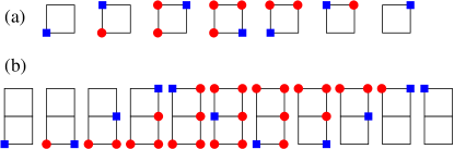
Figure 1: (Color online) Shortest sequences of repeated hops around closed loops leading to effective 2nd NN (top panel) and 3rd NN (bottom panel) hopping. The hole is marked by a blue square, and the defects (spin flips) it creates or annihilates as it moves are marked by red circles.

In perturbational terms, for $t\ll J=4\bar{\jmath}$, the sequence of hoppings depicted in Fig. 1(a) results in 2nd NN hopping $t_{2}=t^{6}/(6^{2}\cdot 10^{2}\cdot 12\bar{\jmath}^{5})$, since the initial and final states, which are both in the no-defect manifold, are connected through 6 hopping processes, and the five intermediary states have energies higher by $6\bar{\jmath},10\bar{\jmath},12\bar{\jmath},10\bar{\jmath},6\bar{\jmath}$ respectively. Similarly, Fig. 1(b) gives a contribution to 3rd NN hopping $t_{3}=t^{10}/(6^{2}\cdot 10^{2}\cdot 14^{2}\cdot 18^{3}\bar{\jmath}^{9})$, as the longer strings of defects are more costly.

Note that clockwise hopping of the hole around the same loop as shown in Fig. 1(b) would generate a higher-order contribution to the 2nd NN hopping $t_{2}^{\prime}\approx t_{3}$ because some of the intermediary states have slightly different energies. This allows us to estimate the range where perturbation theory is valid. If we ask that $t_{2}^{\prime}/t_{2}\leq 0.1$, so that this correction from 5-defect processes to the 3-defect result is small, we find $t\leq 8.4\bar{\jmath}=2.1J$. In other words, because of the relatively long and thus energetically costly loops of flipped spins involved in generating the effective hoppings, perturbation theory extends up to rather large values $t\leq 2J$. For comparison, in cuprates it is believed that $t\sim J/3$, so they would be just outside the perturbational range (for these values, $t_{2}^{\prime}\sim 0.4t_{2}$). Of course, the effects of spin fluctuations cannot be ignored in the cuprates.

Clearly, then, for $t\leq 2J$ the dominant contribution to the hole’s dynamics comes from the processes of Fig. 1(a). We therefore begin by calculating $G(\mathbf{k},\omega)$ in a variational approach, by only allowing such short loops (with up to 3 defects on 3 corners on a square plaquette) to be generated. Longer loops are more expensive and the probability to generate them should be lower. Of course, they can be included in a numerical calculation, but this will lead to only quantitative, not qualitative changes (see below).

The method we use is similar to that used in Refs. Edwards et al., 2010; Alvermann et al., 2010 for the 1D, and in Ref. Berciu and Fehske, 2010 for the 2D Edwards model. Within this variational approximation, we generate the equations of motion for the propagator by using repeatedly the Dyson identity

$$\hat{G}(\omega)=\hat{G}_{0}(\omega)+\hat{G}(\omega)V\hat{G}_{0}(\omega)\,,$$ (9)

where $\hat{G}_{0}(\omega)$ is the resolvent for ${\cal H}_{0}={\cal H}_{\rm AFM}$, while $V$ is the first term in Eq. (5), describing the hopping of the hole. We then find

$$G(\mathbf{k},\omega)=G_{0}(\omega-4\bar{\jmath})\Big{[}1-t\sum_{\bm{\delta}}F_{1}(\mathbf{k},\omega,{\bm{\delta}})\Big{]}\,,$$ (10)

where $G_{0}(\omega)=1/(\omega+i\eta)$, $4\bar{\jmath}$ is the cost of having only the hole in the system (first state in Fig. 1(a)), and $\bm{\delta}$ points to any of the four NN sites, i.e. ${\bm{\bm{\delta}}}\in\{(\pm 1,0),(0,\pm 1)\}$ for a lattice constant $a=1$. The new propagators are

$$F_{1}(\mathbf{k},\omega,\bm{\delta})={1\over\sqrt{N}}\sum_{i\in A}e^{i\mathbf{k}\cdot\mathbf{R}_{i}}\langle{\rm GS}|h_{\mathbf{k}}\hat{G}(\omega)d^{\dagger}_{i}h^{\dagger}_{i+\bm{\delta}}|{\rm GS}\rangle\,,$$ (11)

and are related to the amplitude of probability to propagate between a no-defect state and a 1-defect state such as the second state shown in Fig. 1(a), with a defect at the original site. In the following, for simplicity we will denote $F_{1}(\mathbf{k},\omega,\bm{\delta})$ as $F_{1}(\bm{\delta})$.

An equation of motion for $F_{1}$ can now be generated. The hopping $V$ can lead to three different outcomes: either the hole hops back to site $i$, removing the defect; or it hops by another $\bm{\delta}$, creating a linear string of the type $d^{\dagger}_{i}d^{\dagger}_{i+\bm{\delta}}h^{\dagger}_{i+2\bm{\delta}}|{\rm GS}\rangle$; or it hops by one of the two $\bm{\delta}^{\prime}\perp\bm{\delta}$, leading to a state such as the 3rd state shown in Fig. 1(a). Only the first and last outcomes are allowed within our variational calculation, leading to

$$F_{1}(\bm{\delta}_{1})=-tG_{0}(\omega-10\bar{\jmath})\left[G(\mathbf{k},\omega)+\sum_{\bm{\delta}_{2}\perp\bm{\delta}_{1}}F_{2}(\bm{\delta}_{1},\bm{\delta}_{2})\right]\,,$$ (12)

where

$$F_{2}(\bm{\delta}_{1},\bm{\delta}_{2})=\sum_{i\in A}{e^{i\mathbf{k}\cdot\mathbf{R}_{i}}\over\sqrt{N}}\langle{\rm GS}|h_{\mathbf{k}}\hat{G}(\omega)d^{\dagger}_{i}d^{\dagger}_{i+\bm{\delta}_{1}}h^{\dagger}_{i+\bm{\delta}_{1}+\bm{\delta}_{2}}|{\rm GS}\rangle$$ (13)

describes generalized Green’s functions associated with 2-defect states. Its equation of motion, within our variational space, is

$$F_{2}(\bm{\delta}_{1},\bm{\delta}_{2})=-tG_{0}(\omega-14\bar{\jmath})\left[F_{1}(\bm{\delta}_{1})+F_{3}(\bm{\delta}_{1},\bm{\delta}_{2},-\bm{\delta}_{1})\right]\,,$$ (14)

where

$$F_{3}(\bm{\delta}_{1},\bm{\delta}_{2},\bm{\delta}_{3})=\sum_{i\in A}{e^{i\mathbf{k}\cdot\mathbf{R}_{i}}\over\sqrt{N}}\langle{\rm GS}|h_{\mathbf{k}}\hat{G}(\omega)d^{\dagger}_{i}d^{\dagger}_{i+\bm{\delta}_{1}}d^{\dagger}_{i+\bm{\delta}_{1}+\bm{\delta}_{2}}h^{\dagger}_{i+\bm{\delta}_{1}+\bm{\delta}_{2}+\bm{\delta}_{3}}|{\rm GS}\rangle$$ (15)

describes states with a string of three consecutive defects. Only states such as shown in the middle panel of Fig. 1(a) are in our variational space, hence the unique $F_{3}$ term in the equation of $F_{2}$. Finally, the equation for $F_{3}$ is now connected to two possible 2-defect states. The hole could either hop back, linking to $F_{2}(\bm{\delta}_{1},\bm{\delta}_{2})$, or it could complete the closed loop by hopping to site $i$ and removing the defect that was there, resulting in

$$\sum_{i\in A}{e^{i\mathbf{k}\cdot\mathbf{R}_{i}}\over\sqrt{N}}\langle{\rm GS}|h_{\mathbf{k}}\hat{G}(\omega)h^{\dagger}_{i}d^{\dagger}_{i+\bm{\delta}_{1}}d^{\dagger}_{i+\bm{\delta}_{1}+\bm{\delta}_{2}}|{\rm GS}\rangle=e^{-i\mathbf{k}(\bm{\delta}_{1}+\bm{\delta}_{2})}F_{2}(-\bm{\delta}_{2},-\bm{\delta}_{1})\,.$$ (16)

Eq. (16) follows after a translation by $-(\bm{\delta}_{1}+\bm{\delta}_{2})$, which maintains the site $i$ on the same original sublattice $A$, since $\bm{\delta}_{2}\perp\bm{\delta}_{1}$. Of course, hopping also links $F_{3}$ to two generalized propagators $F_{4}$ with 4 defects, however those are ignored in this 3-defect variational space. Thus, we find:

$$F_{3}(\bm{\delta}_{1},\bm{\delta}_{2},-\bm{\delta}_{1})=-tG_{0}(\omega-16\bar{\jmath})\left[F_{2}(\bm{\delta}_{1},\bm{\delta}_{2})+e^{-i\mathbf{k}\cdot(\bm{\delta}_{1}+\bm{\delta}_{2})}F_{2}(-\bm{\delta}_{2},-\bm{\delta}_{1})\right]\,.$$ (17)

In other words we have a closed system of linear equations for $G$ and the various allowed $F_{1},F_{2},F_{3}$ functions.

This system can be solved analytically. The final result is

$$G(\mathbf{k},\omega)=\frac{1}{\omega+i\eta-\epsilon_{0}(\omega)+4t_{2}(\omega)\cos k_{x}\cos k_{y}+4t_{3}(\omega)\,[\cos(2k_{x})+\cos(2k_{y})]}\,,$$ (18)

where

$$\epsilon_{0}(\omega)=4\bar{\jmath}+4t^{2}G_{0}({\tilde{\tilde{\omega}}})-4t_{3}\,,$$ (19)

$$t_{2}(\omega)=-\frac{2t^{2}G_{0}({\tilde{\tilde{\omega}}})\beta(\omega)}{1-4\beta^{2}(\omega)}\,,$$ (20)

$$t_{3}(\omega)=\beta(\omega)t_{2}(\omega)\,.$$ (21)

The functions that appear in these definitions are:

$$\beta(\omega)=\frac{t^{2}G_{0}({\tilde{\omega}})G_{0}({\tilde{\tilde{\omega}}})\gamma(\omega)}{1-\gamma^{2}(\omega)}\,,$$ (22)

$${\tilde{\tilde{\omega}}}=\omega-10\bar{\jmath}-\frac{2t^{2}G_{0}({\tilde{\omega}})}{1-\gamma^{2}(\omega)}\,,$$ (23)

$$\gamma(\omega)=t^{2}G_{0}({\tilde{\omega}})G_{0}(\omega-16\bar{\jmath}),$$ (24)

and

$${\tilde{\omega}}=\omega-14\bar{\jmath}-t^{2}G_{0}(\omega-16\bar{\jmath})\,.$$ (25)

The Green’s function of Eq. (18) describes a free particle on the $A$ sublattice, with an onsite energy $\epsilon_{0}$, and hoppings $t_{2}$ and $t_{3}$ that correspond to NN and 2nd NN for sites on this sublattice. Interestingly, all these effective quantities are functions of $\omega$, in other words retardation effects are explicitly taken into consideration in this variational calculation. For $t\ll\bar{\jmath}$ we find that indeed $\epsilon_{0}\approx 4\bar{\jmath}-4t^{2}/6\bar{\jmath}$, while $t_{2}=t^{6}/(21600\bar{\jmath}^{5})$. This is precisely twice the value we estimated for Fig. 1(a); the factor of 2 is due to contributions from both clockwise and anticlockwise loops.

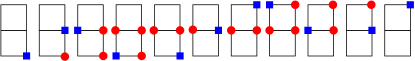
Figure 2: (Color online) An effective $t_{3}$ process generated with only 3-defect strings.

The appearance of the $t_{3}$ term at this level of the calculation is surprising at first, since configurations with 5 defects like that appearing in Fig. 1(b) are not allowed in this variational space. The answer for how to achieve $t_{3}$ hopping with only 3-defect loops is shown in Fig. 2: essentially, instead of removing the last defect at the 6th hopping, another 3-defect process is initiated. It is straightforward to check that in the perturbational limit, the ratio between the expected values for this $t_{3}$ and the $t_{2}$ of Fig. 1(a) is of $t^{4}/(7200\bar{\jmath}^{4})$. This is precisely the ground-state value of $\beta(\omega=4\bar{\jmath})$ in this asymptotic limit, which further validates this statement. It is also now clear that this strategy of starting a new loop when only a single defect is left can be repeated an arbitrary number of times, and an infinite sequence of higher order contributions to $t_{2}$ and $t_{3}$ can be generated this way. This explains the $1-4\beta^{2}(\omega)$ denominators in Eqs. (20),(21), showing that our variational calculation sums contributions from these 3-defect processes to all orders.

As argued previously, the contribution of 5-defect loops is negligible if $t\leq 2J=8\bar{\jmath}$. Interestingly, for such values $2\beta\sim t^{4}/(3600\bar{\jmath}^{4})$ varies from 0 to just above 1 (however, this ignores the change in $\beta(\omega)$ because the ground-state energy moves away from $\omega=4\bar{\jmath}$, as $t/J$ increases). In other words, the denominators in Eqs. (20), (21) could become very small, implying that significant hopping, and thus light effective masses, may be possible in such systems even for rather small $t/J$ ratios.

As a final comment, the fact that $\mathbf{k}$-dependence appears only in the equation for $F_{3}$ confirms that the effective hopping terms are due to completely circling around the closed loops. If we truncated the variational space to include only 2-defect states, which would mean setting $F_{3}\rightarrow 0$ in Eq. (14), the result would be just a renormalization of the on-site energy but no dispersion.

III.2 Hole propagation when $B\neq 0$

Since the dispersion of the hole is due to Trugman loops, it is interesting to consider what happens when a transverse magnetic field $B$ is applied. Because of the large number of elementary hopping processes involved in generating effective longer ranged hoppings, one would expect the phases associated with these effective hoppings to be different from the normal Peierls phase. Put it another way, one would expect Aharonov-Bohm-like interference between clockwise and counterclockwise contributions, over and above the usual Peierls phases, and therefore a spectrum that is not simply that of a bare particle with hoppings $t_{2},t_{3}$ placed in a magnetic field.

Let $\Phi=Ba^{2}$ be the magnetic flux through the elementary square plaquette. Because the dressed hole only lives on one sublattice (sublattice $A$ in our calculation), the actual relevant flux is $2Ba^{2}$, since the unit cell for the sublattice is doubled in size.

From elementary considerations of the Hofstadter butterfly,Hofstadter (1976) we know that we need to consider the cases when the ratio between the magnetic flux and the elementary flux $\Phi_{0}=h/e$ is $2Ba^{2}/\Phi_{0}=p/n$, where $p$ and $n$ are mutually prime integers. In this case, we expect the spectrum to split into $n$ magnetic subbands. Of course, then, the Brillouin zone is folded down $n$ times. We are therefore interested in the spectrum of the dressed hole when

$$\frac{\Phi}{\Phi_{0}}={p\over 2n}$$ (26)

(for simplicity of notation, we also introduce $\phi=2\pi\Phi/\Phi_{0}=\pi p/n$).

We use the Landau gauge $\mathbf{A}({\mathbf{r}})=Bx\mathbf{e}_{y}$, in which case only the hopping integrals in the $y$-direction acquire Peierls phases. The magnetic unit cell will contain $2n$ sublattice $A$ sites, and it is drawn, together with the Peierls phases, in Fig. 3. Each site in the unit cell is labeled by the index $\alpha=0,\ldots,2n-1$ which establishes its location in the unit cell, as well as the phase associated with hopping off this site in the positive $y$-direction.

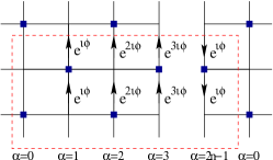
Figure 3: (Color online) Magnetic unit cell in real space when $\phi=2\pi p/(2n)$, where $p$ and $n$ are mutually prime integers. The unit cell is marked by the red dashed line, and contains $2n$ sites, labeled by squares, on the $A$ sublattice. These are indexed by their corresponding $\alpha=0,...,2n-1$. The value of $\alpha$ also appears in the Peierls phases for hopping in the direction of the arrow.

The Hamiltonian is identical to that of Eq. (1), with the proper phases included in the hoppings. Of course, we assume that the magnetic field is not sufficiently large to overcome the AFM coupling and favor a FM ground state. Also, we ignore the Zeeman term – since the spins are reshuffled as the hole hops around, the total $z$-axis spin $S_{z}=\sum_{i}\sigma_{i,z}$ remains constant and therefore the Zeeman contribution is an overall constant.

We now need to introduce $2n$ distinct plane waves, associated with each site of the unit cell

$$h^{\dagger}_{\alpha,\mathbf{k}}=\sqrt{{2n\over\bar{N}}}\sum_{i\in A_{\alpha}}e^{i\mathbf{k}\cdot\mathbf{R}_{i}}c_{i\uparrow}\,,$$ (27)

where $A_{\alpha}$ collects all sites on sublattice $A$ with the same value of $\alpha$. The procedure to generate the equations of motion for the propagator

$$G_{\alpha^{\prime}\alpha}(\mathbf{k},\omega)=\langle{\rm GS}|h_{\alpha^{\prime},\mathbf{k}}\hat{G}(\omega)h^{\dagger}_{\alpha,\mathbf{k}}|{\rm GS}\rangle$$ (28)

is just as before, however now one has to take into consideration the Peierls phases. These can either be included in the definition of the new $F_{1},F_{2},F_{3},$ functions, or can be explicitly pulled out. In either case, the overall structure of the system of linear equations is very similar to that in the $B=0$ case, and can be solved similarly. This allows us to reduce it to a single equation involving only $G$ functions, which reads:

$$G_{\alpha^{\prime}\alpha}(\mathbf{k},\omega)=G_{0}(\omega-\tilde{\epsilon}_{0})\left\{\delta_{\alpha^{\prime}\alpha}-\tilde{t}_{2}\left[2\cos(k_{y}-(\alpha-\tfrac{1}{2})\phi)e^{ik_{x}}G_{\alpha^{\prime},\alpha-1}(\mathbf{k},\omega)+2\cos(k_{y}-(\alpha+\tfrac{1}{2})\phi)e^{-ik_{x}}G_{\alpha^{\prime},\alpha+1}(\mathbf{k},\omega)\right]\right.\\ \left.-\tilde{t}_{3}\left[e^{2ik_{x}}G_{\alpha^{\prime},\alpha-2}(\mathbf{k},\omega)+2\cos(2k_{y}-2\alpha\phi)G_{\alpha^{\prime}\alpha}(\mathbf{k},\omega)+e^{-2ik_{x}}G_{\alpha^{\prime},\alpha+2}(\mathbf{k},\omega)\right]\right\}\,.$$ (29)

Here we used the short-hand notations:

$$\tilde{\epsilon}_{0}\equiv\epsilon_{0}(\phi,\omega)=4\bar{\jmath}+\frac{4t^{2}G_{0}({\tilde{\tilde{\omega}}})(1-2\beta^{2}(\omega))}{1-4\beta^{2}(\omega)+4\beta^{4}(\omega)\sin^{2}(2\phi)}\,,$$ (30)

$$\tilde{t}_{2}\equiv t_{2}(\phi,\omega)=-\frac{2t^{2}G_{0}({\tilde{\tilde{\omega}}})\beta(\omega)\left[(1-\beta^{2}(\omega))\cos{3\phi\over 2}+\beta^{2}(\omega)\cos{5\phi\over 2}\right]}{1-4\beta^{2}(\omega)+4\beta^{4}(\omega)\sin^{2}(2\phi)}\,,$$ (31)

and

$$\tilde{t}_{3}\equiv t_{3}(\phi,\omega)=-\frac{2t^{2}G_{0}({\tilde{\tilde{\omega}}})\beta^{2}(\omega)\cos(2\phi)}{1-4\beta^{2}(\omega)+4\beta^{4}(\omega)\sin^{2}(2\phi)}\,.$$ (32)

Remarkably, Eq. (29) is identical to the equation of motion one would obtain for the propagator associated with a Hamiltonian on the sublattice $A$ only, with an on-site energy $\tilde{\epsilon}_{0}$ and NN and 2nd NN hopping (as defined on the sublattice) given by $\tilde{t}_{2},\tilde{t}_{3}$, plus the proper Peierls phases for the applied magnetic field. The terms in the parenthesis multiplied by $\tilde{t}_{2}$ come from NN hopping by $\pm\delta_{x}\pm\delta_{y}$, with the proper Peierls phases accounted for in the phases of the cosine functions; similarly, the terms in the parenthesis multiplied by $\tilde{t}_{3}$ come from next-NN hopping by $\pm 2\delta_{x},\pm 2\delta_{y}$. Only the $\pm 2\delta_{y}$ hopping accumulates a Peierls phase, in this case, hence the cosine term appears only for that term.

It follows that $\tilde{\epsilon}_{0},\tilde{t}_{2}$ and $\tilde{t}_{3}$ are the effective parameters describing the new quasiparticle (the dressed hole in the Néel AFM background plus magnetic field). They depend strongly on the magnetic field, besides the $\omega$-dependence due to retardation effects. As expected, they have the correct values when $\phi\rightarrow 0$, as given by Eqs. (19)-(21).

The $\cos{3\phi\over 2}$ and $\cos{5\phi\over 2}$ terms in $\tilde{t}_{2}$, respectively $\cos{2\phi}$ term in $\tilde{t}_{3}$, are due to Aharonov-Bohm interference between clockwise and counterclockwise loops. This can be checked directly in the asymptotic limit $t\ll J$ by counting the accumulated Peierls phases for the processes from Figs. 1(a) and 2. Because of these, we expect the resulting Hofstadter butterfly to have an unusual periodicity.

That is, we still expect the appearance of $n$ bands when $2\Phi/\Phi_{0}=p/n$, due to interference between the Peierls phases. However, additional dependence of the hoppings on $\phi$ because of the Aharonov-Bohm interference will further modulate the overall bandwidth with a period $2\pi$ in $\phi$ (the band structure is invariant if only $t_{2}$ changes its sign). In contrast, normally, (i.e. for constant $\epsilon_{0},t_{2},t_{3}$) the spectrum is an even function of $\phi$ with period $\pi$, because if the magnetic flux through the unit cell ($2\Phi$, in this case), increases by $\Phi_{0}$, the spectrum stays unchanged. Thus, we expect a quite different-looking Hofstadter butterfly for the dressed hole. In particular, since at least for small $t/J$ we expect $t_{3}\ll t_{2}$, the spectrum should become extremely narrow every time $\tilde{t}_{2}\rightarrow 0$ because of destructive Aharonov-Bohm interference.

III.3 Numerical calculation method

The numerical calculation that we describe in this section has been carried out only for the case $B=0$. This is a straightforward generalization of the 3-defect variational calculation discussed above. The idea is to systematically increase the size of the variational space, to see whether addition of configurations with longer loops of defects changes results significantly. If it does not, then we know that the calculation is converged and therefore the results are essentially exact.

We use an index $N$ to characterize the maximum number of defects allowed within the variational subspace. The equations of motion are generated as before, starting from just the hole and keeping all configurations linked to by hole hopping, up to those involving $N$ defects. The exception is for longer chains with $N\geq 4$ defects, where we do not allow the chain to “self-cross” itself. For instance, for the 6-defect chain sketched in Fig. 4, the hole is not allowed to hop either left or down. Either of these processes would result in a configuration with the hole having two strings of defects attached to it. Trying to remove all these defects involves a very complicated sequence of Trugman loops, and is therefore expected to have a very small contribution to $t_{2}$ and $t_{3}$. The other role of such configurations is to renormalize energies, but as we will see in the next section, we can argue that their effect must be quite negligible.

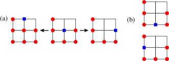
Figure 4: (Color online) Examples of discarded configurations: (a) the central 6-defect configuration is only allowed to be linked back to the 5-defect configuration that generated it, shown to its right, or to the 7-defect configuration shown to its left. The other two “self-crossing” 5-defect configurations shown in (b) are not kept in the variational space.

This is why for a configuration like that of Fig. 4, we allow the hole only to hop back (towards right) to the $F_{5}$ configuration from which it derived; or to hop up to generate a $F_{7}$ configuration. In its turn, hopping to the left from this $F_{7}$ configuration will close the loop and give a new contribution to the effective $t_{2}$. New possible closed loops (and therefore additional contributions to $t_{2},t_{3}$) appear for $N=3,5,7,\ldots$

Once all the allowed configurations have been generated for a given $N$, the resulting (very sparse) linear system comprising their equations of motion is solved numerically using PARDISO.Schenk and Gärtner (2004); *SG06 We show results with up to $N=7$, in the following, because here there are already over ten thousand allowed configurations, and, as we will see, this is sufficiently large for convergence to be achieved up to a quite high $t/J$ ratio.

Finally, note that in the numerical calculation, $N=3$ contains many more configurations than in the $N=3$ analytical calculation, because now all possible 2- and 3-defect configurations (not just those like in Fig. 1(a)) are included. The results of the two methods, therefore, should not be expected to be identical.

IV Results

IV.1 $B=0$ case

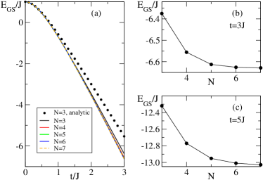
Figure 5: (Color online) (a) GS energy vs. $t/J$, as predicted by the analytic solution (circles) and numerically in the variational spaces with $N=3,...,7$; (b) and (c) show the dependence on $N$ of the GS energy for $t/J=3$, respectively 5.

We begin by looking at the ground-state (GS) energy as a function of $t/J$, using both the analytical and the numerical methods. Results are shown in Fig. 5(a) for $t/J\leq 3$. As expected, in the limit $t/J\rightarrow 0$, all curves converge towards $E_{\rm GS}=J=4\bar{\jmath}$, which is the cost of placing the hole in the lattice (breaking four AFM exchange bonds). As $t$ increases and the hole acquires a finite mass, its energy is lowered. For small $t/J$, all values are in excellent agreement, but for larger $t/J$ they begin to fan out. At $t/J=3$, convergence has already been achieved for $N=7$, as shown in Fig. 5(b). For $t/J=5$, $N=7$ is not yet fully converged, although further corrections are not expected to be large. Note that we do not show results up to $t/J=5$ in panel (a) because the corresponding increase of the energy range to be displayed makes it even more difficult to distinguish the numerical curves from one another.

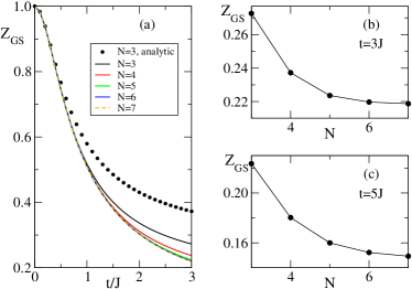
Figure 6: (Color online) Same as in Fig. 5, but for the GS quasiparticle weight instead of GS energy.

The analytical calculation indeed gives a reasonably accurate value up to $t/J\sim 1\ldots 2$. The fact that the biggest variation is between it and the $N=3$ numerical calculation, means that the 2- and 3-defect configurations ignored in the analytical approximation play a significant role in renormalizing the overall energy. This is not surprising, since these are some of the least expensive configurations. However, qualitatively and even quantitatively it is clear that this analytical approximation is quite good up to fairly large $t/J$ values.

The quasiparticle weight

$$Z({\mathbf{k}})=|\langle\phi_{\mathbf{k}}|h^{\dagger}_{\mathbf{k}}|{\rm GS}\rangle|^{2}\,,$$ (33)

defined as the overlap between the lowest eigenstate at a given momentum,

$${\cal H}|\phi_{\mathbf{k}}\rangle=E({\mathbf{k}})|\phi_{\mathbf{k}}\rangle\,,$$ (34)

and the non-interacting state $h^{\dagger}_{\mathbf{k}}|{\rm GS}\rangle$, is shown at ${\mathbf{k}}=0$ in Fig. 6. It remains quite considerable even for large $t/J$, showing that a significant part of the wavefunction consists of the hole alone, with no strings of defects. The effect of increasing the variational space is more visible here, as expected due to normalization: as the wavefunction acquires extra components in a larger variational space, the weight of the hole-only part decreases, even if overall the energy of the state is not much changed.

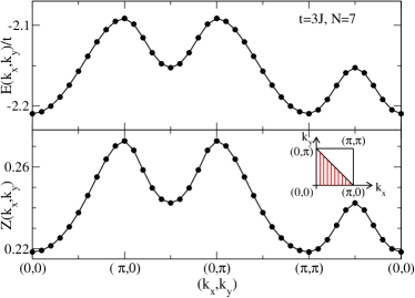
Figure 7: (Color online) Energy $E({\mathbf{k}})/t$ (upper panel) and quasiparticle weight $Z({\mathbf{k}})$ (lower panel) along the high-symmetry directions of the square lattice Brillouin zone, for $t/J=3$ and $N=7$. The inset in the bottom panel shows the upper right quadrant of the full Brillouin zone; the AFM Brillouin zone is shaded. Lines are guides to the eye.

The hole band dispersion $E({\mathbf{k}})$ and quasiparticle weight $Z({\mathbf{k}})$ are shown in Fig. 7, along high-symmetry cuts in the Brillouin zone of the original square lattice, for $t/J=3,N=7$. The band folding due to the AFM order is clearly apparent. These results are very similar to those found for comparable parameters in the 2D Edwards model (see Fig. 10 of Ref. Berciu and Fehske, 2010): the minimum is at ${\mathbf{k}}=(0,0)$, and ${\mathbf{k}}=({\pi\over 2},{\pi\over 2})$ is a saddle point (unlike in cuprates, where it is the actual minimum). The quasiparticle weight is fairly constant but with local variations that mimic the shape of the dispersion. This similarity is not surprising; even though the Edwards model allows more states (e.g. with more defects at a site), those are higher in energy and do not contribute much to the GS. The mechanism for generating an effective mass is identical in both models, with only small quantitative differences due to the energy assigned to the strings of defects in the two models.

One difference between the two models is illustrated in Fig. 8, where we show the dispersion for $N=3,5,7$ and $t/J=3$ along fewer cuts. The symbols are data from the numerical simulations, and the lines are fits to an effective dispersion

$$E^{*}({\mathbf{k}})=E_{0}-4t_{2}^{*}\cos k_{x}\cos k_{y}-2t_{3}^{*}\left[\cos(2k_{x})+\cos(2k_{y})\right],$$ (35)

along the $(0,0)\rightarrow(0,\pi)$ line. Using the same parameters along the $(0,0)\rightarrow(\pi,\pi)$ line is clearly not a good fit. In contrast, for the Edwards model such fits worked well in the entire Brillouin zone. This suggests that the retardation effects may be somewhat stronger in this case: even though we know that only $t_{2}(\omega)$ and $t_{3}(\omega)$ effective hoppings are generated, these may not be well approximated by constant values $t_{2}^{*},t_{3}^{*}$ if the $\omega$ dependence is considerable within the bandwidth of the dressed hole.

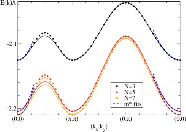
Figure 8: (Color online) Dressed hole dispersion $E(\mathbf{k})/t$ along high-symmetry cuts in the Brillouin zone, for $t/J=3$ and $N=3,5,7$. Symbols are numerical data (for $N=7$, same as in Fig. 7) and lines are results to a fit as in Eq. (35), with parameters extracted for best fit on the $(0,0)-(\pi,0)$ cut. Dashed lines are fits to extract the effective mass.

This is less of an issue at smaller $t/J$, where the bandwidth is significantly narrower. In fact, even for $t/J=3$, the results for $N=3$ shown in Fig. 8 clearly have a smaller bandwidth than for $N=5,7$. This is not surprising, since longer loops with additional contributions to effective hoppings are included in the latter cases. Even though the decrease in bandwidth is not that large, it is clear that the fit is better for the $N=3$ case. This may explain why the fit worked well for the 2D Edwards model,Berciu and Fehske (2010) where the solution was restricted to $N=3$ and the bandwidths were narrower also due to more costly defects (equivalent to larger $J$) than in Fig. 8.

Since we cannot extract meaningful $t_{2}^{*},t_{3}^{*}$ values, we instead calculate the effective mass

$$\left[\frac{1}{m^{*}}\right]_{x,y}=\left.\frac{\partial^{2}E({\bf k})}{\partial k_{x}\partial k_{y}}\right|_{|{\bf k}|\to 0}\,,$$ (36)

with fits as shown by the dashed lines in Fig. 8. As expected, the mass is found to be isotropic. The results are shown in Fig. 9, on a logarithmic scale. The effective mass $m^{*}$ is in units of the band mass $m$, i.e. the bare particle mass if there was no AFM background.

We show results up to $t/J=5$, even though the values are not fully converged for $t/J>3$. At these larger values, longer loops than $N=7$ would need to be included. From results such as in Fig. 5(c), however, we do not expect those further corrections to be very significant. Also, they would decrease $m^{*}$, as they would open additional channels for effective hopping, so the values shown in Fig. 9 can be taken as an upper bound for $m^{*}$.

In the limit $t/J\rightarrow 0$, the effective mass becomes very large. As discussed, from perturbation theory here we expect $t_{2}=t^{6}/(21600\bar{\jmath}^{5})$. The corresponding $m^{*}/m=10.55(J/t)^{5}$ is shown as a dashed line in the inset, in good agreement with the values obtained from the analytical and numerical calculations (symbols and full lines). The effective mass diverges as $t/J\to 0$ since the hole is bound to its original site in this case. As $t/J$ increases, the effective mass decreases significantly, and it reaches $m^{*}/m\sim 40$ for $t/J=3$. Since this decrease is mirrored by the analytical $N=3$ calculation, it must be due to the summation over repeated 3-defect loops, like those shown in Fig. 2. Longer loops further lower the effective mass. The $N=5$ loops give a significant contribution for $t/J>1$, validating the expectations based on perturbation theory. The contribution of the $N=7$ loops is still quite small, for these values. We expect $m^{*}$ to further decrease with increasing $t/J\rightarrow\infty$. However, capturing that limit is very difficult if not outright impossible with this variational formulation, given the huge increase in possible configurations with increasing $N$.

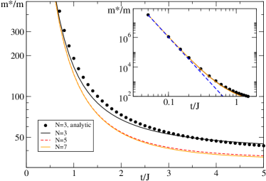
Figure 9: (Color online) Effective mass vs. $t/J$. The inset shows the same data, plus the prediction of the weak-coupling perturbation theory (dashed line).

The main result, thus far, is that a hole in an Ising AFM is fairly mobile if $t$ and $J$ are comparable, even though there are no spin fluctuations in this model.

IV.2 $B\neq 0$ case

We now proceed to discuss the spectrum of the dressed hole in the presence of a transverse magnetic field $B$. We will use the $N=3$ analytical Eq. (29), and solve it numerically for various values of $\phi=\pi p/n$. We show results for $t/J=3$, even though we know that here the analytical calculation is not sufficient for full convergence, simply because its $B=0$ bandwidth is sufficiently large to make it easier to see the effect of a finite $B$. We note that the numerical calculation in the variational spaces corresponding to various $N$ can be carried out as well, however each previous unknown, corresponding to an allowed configuration of defects, now becomes a $2n\times 2n$ matrix of unknowns, corresponding to each of the $2n$ distinct sites in the magnetic Brillouin zone shown in Fig. 3. This huge increase in the size of the linear system to be solved, especially for larger $n$ values (smaller magnetic fields) makes the implementation of this scheme cumbersome, and unnecessary since we do not expect any qualitative changes.

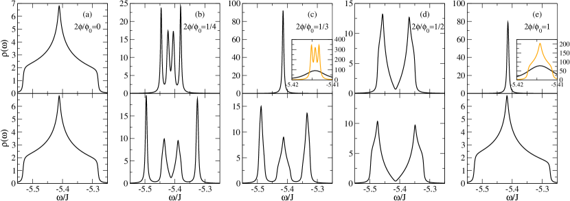
Figure 10: (Color online) Local density of states $\rho(\omega)$ vs. $\omega/J$ for various magnetic fluxes through the sublattice unit cell $2\Phi/\Phi_{0}=0,{1\over 4},{1\over 3},{1\over 2}$ and $1$, for $t/J=3$. The upper panels show the full solution of Eq. (29), while the lower panels show the solution if the Aharonov-Bohm interference is turned off by setting $\phi=0$ in Eqs. (30)-(32). The broadening is $\eta/J=2.5\cdot 10^{-3}$, except for the orange (light) curves in the insets, for which $\eta/J=2.5\cdot 10^{-4}$.

After solving the linear system in Eq. (29), we calculate the local density of states (LDOS)

$$\rho(\omega)=-{1\over\pi}\mbox{Im }\sum_{\mathbf{k}}G_{\alpha\alpha}({\mathbf{k}},\omega),$$ (37)

where the sum is over the (highly folded) magnetic Brillouin zone corresponding to the magnetic unit cell of Fig. 3. This LDOS is independent of the site $\alpha=0,...,2n-1$ used, hence the lack of a site index.

We first consider the effect of the additional dependence on $B$ due to the Aharonov-Bohm interference, on the Hofstadter butterfly expected when the magnetic flux through the unit cell is comparable to $\Phi_{0}$. Results for various simple ratios are shown in Fig. 10. In all cases, the upper panel shows the full results, whereas the lower panel shows the results when the Aharonov-Bohm interference is turned off, i.e. we use the $\phi=0$ values $\epsilon_{0}(\phi=0,\omega)$, $t_{2}(\phi=0,\omega)$ and $t_{3}(\phi=0,\omega)$ in Eq. (29).

For the $B=0$ case shown in (a), the results are of course identical. The density of states resembles that of a 2D square lattice with NN hopping. This is expected, since the dominant hopping term is $t_{2}$, which plays the role of NN hopping for the sublattice on which the dressed hole lives. The LDOS is slightly distorted due to (small) contributions from the $t_{3}$ term and the retardation effects. These small distortions and asymmetries are observed in all other panels.

For a finite flux through the sublattice unit cell $2\Phi/\Phi_{0}=1/n$, the band splits into $n$ subbands, as expected in standard Hofstadter butterfly phenomenology. The bands are not fully separated because we used a broadening $\eta/J=2.5\cdot 10^{-3}$ which, while small, is still comparable with some of these features’ bandwidth. Despite this, the various subbands are easily identifiable.

In Figs. 10 (b) and (d), the full result (top panel), while quite similar in aspect to the lower panel, shows a somewhat narrower bandwidth. This is not surprising, since the Aharonov-Bohm interference terms like $\cos(3\phi/2)$ etc. are responsible for a decrease in the value of the effective hoppings, and therefore of the overall bandwidth. This also explains the apparent “collapse” of the butterfly for $\phi=\pi/3$ and $\phi=\pi$, shown in Figs. 10 (c) and (e), respectively. The very narrow peak seen in both cases shows the expected subband structure, if a much smaller $\eta/J=2.5\cdot 10^{-4}$ values is used, as done in the inset: the former case shows the 3 subbands (these features are so narrow that even this much smaller $\eta$ can only partially resolve them), while the later case shows the one band. The extreme narrowing is due to the Aharonov-Bohm interference, which at these values of the flux results in a very small or vanishing $t_{2}(\phi,\omega)$, see Eq. (31), and a bandwidth set by $t_{3}(\phi,\omega)\ll t_{2}(0,\omega)$.

As already noted, this additional $B$-dependent modulation of the Hofstadter structure, coming from the Aharonov-Bohm interference, is also responsible for an increase in the periodicity of the butterfly. The lower panel shows that, as expected in models with constant hopping integrals, the butterfly is periodic if the flux through the unit cell increases by a flux quantum (here, $2\Phi\rightarrow 2\Phi+\Phi_{0}$, or $\phi\rightarrow\phi+\pi$). The full result clearly does not have this periodicity. As discussed previously, based on Eqs. (30)–(32) we expect the periodicity to be $\phi\rightarrow\phi+2\pi$ for the full Aharonov-Bohm case; our simulations confirm this (not shown).

We can imagine that this $2\pi$ periodicity survives if one allows longer loops in the calculation, but some care is needed. For example, loops like those shown in Fig. 1(b) would bring in factors of $\cos(7\phi/2)$ in their contribution to $t_{2}$, and various other Aharonov-Bohm phases will be associated with longer loops. We calculated several of these and all are consistent with the $2\pi$ periodicity; so we believe this $2\pi$ period is correct to all orders, but do not have a proof.

Finally, we discuss the role of the Aharonov-Bohm interference at very small magnetic fields. In this case, one expects the spectrum to separate in a sequence of Landau levels (LLs) separated by the cyclotron frequency. The appearance of LLs in the spectrum leads to quantum oscillations in various transport measurements, such as de Haas-van Alphen oscillations.

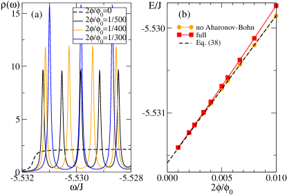
Figure 11: (Color online) (a) LDOS for small magnetic fields (full lines), showing several LLs at the bottom of the spectrum. The dashed lines shows the $B=0$ LDOS; (b) the location of the lowest LL peak, in the full calculation (squares) and with the Aharonov-Bohm interference turned off (circles). The dashed line is the analytical prediction of Eq. (38). These results are for $t/J=3$ and $\eta/J=10^{-5}$.

The LDOS at the lower edge, with (full lines) and without (dashed line) very small magnetic fields applied, is shown in Fig. 11(a). The $B=0$ LDOS shows the jump at the band edge, here smoothed out by a finite $\eta$ value, and the roughly constant 2D density of states above it. The slight monotonic increase is due to the use of a tight-binding dispersion, as opposed to an approximate parabolic one.Berciu and Cook (2010) When the small field is turned on, we see that this LDOS splits into equally spaced narrow peaks, marking the LLs. The cyclotron frequency, defined by the distance between consecutive LLs, increases roughly linearly with $B$, and so does the weight in each LLs, as expected because of its larger degeneracy.

In Fig. 11(b), we plot the energy of the lowest LL against the flux through the unit cell. Squares show the full result, while circles are the result when the Aharonov-Bohm oscillations are turned off. The dashed line shows the value of the lowest LL for a particle of constant mass $m^{*}$,

$$\varepsilon=[E_{\rm GS}+\hbar\omega_{c}/2]/J\,,$$ (38)

where the cyclotron frequency is $\omega_{c}=eB/m^{*}$, and $E_{\rm GS}$ and $m^{*}$ are the $B=0$ values of the dressed hole ground-state energy and effective mass, respectively. This prediction is in excellent agreement with the results where the Aharonov-Bohm interference is turned off. In contrast, the full results show additional quadratic $B$-dependence. This is not so surprising, since for small magnetic fields, the effective hoppings depend quadratically on $B$ through the Aharonov-Bohm interference terms, and one would expect that dependence to be mirrored here through the effective mass.

We do not perform a more quantitative analysis because, as already mentioned, the $N=3$ analytical case is not fully converged at this value of $t/J=3$; for example, the effective mass is $m^{*}/m\approx 54$, whereas the converged result is $m^{*}/m\approx 40$ – this is quite a sizable difference. Going to a smaller $t/J$ is not easy either, because the bandwidth narrows (or, equally, the effective mass increases) and it becomes more and more difficult to separate various features.

V Summary

To conclude, we have investigated the motion of a hole in a 2D square Ising AFM. We showed that summation of the contribution of all Trugman loops up to a given length $N$ can be carried out numerically, and convergence is reached for $N=7$ if $t/J\lesssim 3$. Qualitatively correct and quantitatively quite reasonably accurate results are obtained from a simple analytical approximation for $N=3$. We find that the effective mass of the hole can be fairly low, of around 30…40 $m$, if $t/J\sim$ 3…5.

If a magnetic field is turned on, Aharonov-Bohm interference between clockwise and counterclockwise Trugman loops leads to dependence of the effective hoppings on the magnetic field over and above the usual Peierls phases. Their most spectacular manifestation is in the “collapse” of the Hofstadter butterfly structure at fields where the Aharonov-Bohm interference is destructive. Of course, creating large enough magnetic fields to see the Hofstadter butterfly band structure in a crystal is still a challenge (moreover, one would need a large $J$ in order to prevent a transition to ferromagnet order, at such large fields). Nevertheless, this is an interesting effect that might be mimicked in some other type of systems.

For small magnetic fields, where the magnetic length is large as compared to the unit cell, Landau levels form. Here, we find that the effect of the Aharonov-Bohm phases is to bring additional dependence on $B$ through $m^{*}(B)$, in the cyclotron frequency. This is a small effect, but one that might be easier to see through various quantum oscillations-type measurements.