Confinement induced resonances in anharmonic waveguides

Abstract

We develop the theory of anharmonic confinement-induced resonances (ACIR). These are caused by anharmonic excitation of the transverse motion of the center of mass (COM) of two bound atoms in a waveguide. As the transverse confinement becomes anisotropic, we find that the COM resonant solutions split for a quasi-1D system, in agreement with recent experiments. This is not found in harmonic confinement theories. A new resonance appears for repulsive couplings ($a_{3D}>0$) for a quasi-2D system, which is also not seen with harmonic confinement. After inclusion of anharmonic energy corrections within perturbation theory, we find that these ACIR resonances agree extremely well with anomalous 1D and 2D confinement induced resonance positions observed in recent experiments. Multiple even and odd order transverse ACIR resonances are identified in experimental data, including up to $N=4$ transverse COM quantum numbers.

I introduction

Ultra-cold low-dimensional atomic gases show unique quantum properties, and have attracted a great deal of interest. For a one-dimensional (1D) Bose gasGirardeau1960 ; LiebLiniger1963 ; Yang1969 , the finite-temperature correlations predicted for a Tonks-Girardeau gasGangardt ; 1DCorrelations have been experimentally verifiedTolra-NIST-exp ; Weiss-exp , and a cross-over to a non-equilibrium super Tonks-Girardeau gas has been realized Haller2009R . For a two-dimensional (2D) geometry, the Berezinskii-Kosterlitz-Thouless phase transition was predicted Berezins1971D ; Kosterlitz1973O , and subsequently observed in experiment Hadzibabic2006B . In these experiments, one or two spatial degrees of freedom are removed by introducing tight confinement via an optical lattice or a tightly focused anisotropic dipole trap.

Atomic interactions can also be tuned precisely by means of a molecular Feshbach resonance in an external magnetic field Feshbach1962A ; Kohler2006P ; Bloch2008M . This allows an effective contact interaction with scattering length $a_{3D}$ to be created, with scattering lengths that can be varied over a wide range of positive and negative values. Owing to these methods, low-dimensional atomic gases now provide a high degree of control for tests of fundamental many-body physics in reduced dimensions. These systems are often much simpler than condensed matter physics experiments, which have complex crystal structure, interactions and disorder.

Confinement-induced resonances (CIR) are one of the most intriguing phenomena found in low-dimensional systems. These were first predicted theoretically by Olshanii Olshanii1998A , who considered a two-body S-wave scattering problem in a quasi-1D trap with cylindrically symmetric transverse harmonic confinement. The CIR can be understood as a novel type of Feshbach resonance, where the transverse ground mode and the manifold of molecular internally excited modes play the roles of the open and closed channels respectively Bergeman2003A . Related effects occur in mixed dimensional traps Nishida ; Lamporesi . A direct generalization of Olshanii’s theory to anisotropic transverse confinement shows that there is only one harmonic CIR (HCIR) resonance, no matter how large the transverse anisotropy Peng2010C . For large anisotropy, this theory crosses over smoothly to the case of a quasi-2D trap, where a single HCIR occurs with a negative S-wave scattering length, $a_{3D}<0$ Petrov2000B ; Petrov2001I ; Naidon2007E .

There have been a number of related experimental investigations, which in some cases appear to contradict each other. In the recent Innsbruck $Cs$ experiment with a quasi-1D geometry Haller2010C , two or more resonances were observed as the transverse confinement became more and more anisotropic. For a quasi-2D geometry, some experiments have observed 2D resonances on the attractive side with $a_{3D}<0$ Frohlich2010R , while others have resonances on the repulsive side with $a_{3D}>0$ Haller2010C ; Vale2011 . Both the observation of multiple resonances and 2D resonances with repulsive interactions are in disagreement with standard HCIR predictions Petrov2000B ; Petrov2001I ; Naidon2007E .

In this paper, a detailed explanation is proposed for these anomalous resonances. The mechanism is that the new resonances are due to center-of-mass (COM) excitations of molecules or atom pairs. These have a different character to the excitation of internal molecular degrees of freedom found in the Olshanii approach and its generalizations. The new COM resonances can only become coupled to the input state by anharmonic terms in the trapping potential. Hence, we term these effects anharmonic confinement induced resonances (ACIR). The ACIR resonances cannot occur in harmonic traps due to Kohn’s theorem Kohn . However, they are certainly observable in current ultra-cold atomic physics experiments, which have relatively large anharmonicities.

The coupling of the COM motion to the relative motion gives additional degrees of freedom not found with parabolic traps. This causes a series of additional scattering resonances due to the mixing of COM and relative motion. The nonlinear mixing caused by anharmonic terms in the potential makes these phenomena analogous to frequency-mixing effects found in nonlinear optics. They provide a fundamentally new pairing mechanism, which may lead to new opportunities for quantum engineering in atomic, photonic or acoustic waveguides. Our results are therefore qualitatively different to harmonic CIR. We predict both multiple 1D resonances and 2D resonances with repulsive interactions. Both results are in quantitative agreement with experiment.

We note that this possibility was also envisaged in three earlier papers. In Peano et al Peano , the general idea is addressed, although using a different technique, and for a different type of trap. Kestner and Duan Kestner2010A treat anharmonic resonance in a double well. In a more recent investigation, parallel to our own, Sala et al Saenz have also concluded that the recent Innsbruck experiments provide evidence for ACIR resonances. The main differences in the treatment are that we have accurately calculated the size of the anharmonic resonance shifts, as well as giving quantitative estimates of relevant parameters. We also compare our theory with the observed multiple resonances, including even and odd order COM resonances.

The paper is arranged as follows. We first analyze the types of transverse excitations available, and the operational processes that can lead to the observed resonances (Sec.II). In Sec.III, a Hamiltonian model of nonlinear CIR is presented, by introducing anharmonic perturbations in the Hamiltonian. In Sec.IV, this is analyzed using perturbation theory for the 1D case. The results are compared to experiments on anisotropic traps, showing the observed splitting is well-explained with the anharmonic COM resonance ACIR model. Next, we consider results for the case of large trap anisotropies, and demonstrate that the observed resonances can be quantitatively explained with excellent accuracy by considering multiple resonances with both even and odd order COM transverse quantum numbers. A similar calculation is carried out for a quasi-2D system in Sec. V, which is also compared with experiment. The main results are summarized in Sec.VI.

II Two-body CIR physics

In recent one and two dimensional confinement induced resonance experiments, there are many observed resonances not explained by conventional CIR theory. In two dimensions, resonances are observed for $a_{3D}>0$, (the BEC side of the resonance) which is the opposite to that expected in the usual theory. Similarly, unexplained multiple resonances occur for one-dimensional CIR with anisotropic transverse confinement. These are also not predicted by the simple two-particle model Olshanii1998A with linear confinement. However, the experiments have some features not included in this idealized model, and the obvious question is: which experimental properties are responsible for the additional observed resonances?

II.1 Harmonic CIR solutions

The possible modes of excitation of a pair of atoms in a transverse potential are illustrated in Fig.1. The COM mode is shown in (a), with two atoms moving together. This is not coupled to the atomic ground state in a harmonic trap, due to Kohn’s theorem. The relative motion mode is shown in (b), with an excitation of the relative coordinate. This is the usual harmonic confinement induced resonance in a one dimensional waveguide with a transverse parabolic potential. The HCIR resonance is simply the first internally excited resonance of the two-body ground state.

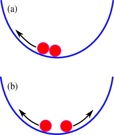
Figure 1: (Color online) (a) Illustration of an ACIR resonance, in which two atoms are driven in a molecule-like excited state with a transverse COM motion in the trap. Both atoms move together, to give a transverse resonance of the COM degree of freedom. This is only coupled to the atomic ground state if the potential is anharmonic. (b) Illustration of an HCIR resonance, in which the atoms move in relative motion, to give an excited state rather like a conventional vibrational excited state of a molecule.

However, there is a subtlety here. Both types of excitation are an adiabatic continuation of the transversely excited free-particle states, as the inter-particle interaction is increased. The free-particle states have both center-of-mass (COM) quantum numbers $N_{x},N_{y},$ and internal quantum numbers, $n_{x},n_{y}$. Therefore, there are a large number of possible excited states that could, in principle, be coupled to the atomic ground state in a Feshbach type of resonance.

In a rotationally symmetric model, both the internal and COM excited states near $2\hbar\omega$ are degenerate in energy, and cannot lead to distinct resonances even if coupled to the incoming states. If there is no rotational symmetry, this degeneracy is broken, leading to the possibility of multiple resonances. Experimentally there is more than one resonance in the recent Innsbruck experiment Haller2010C . Due to the similarity with the HCIR predictions Olshanii1998A , these were initially identified as conventional harmonic CIR resonances, corresponding to excitations of internal degrees of freedom.

However, an analysis of the anisotropic case Peng2010C indicates that internally excited two-body states only give rise to only a single CIR. We note that Kohn’s theorem Kohn prohibits the excitation of COM resonances from incoming states with no transverse momentum, if the confinement is parabolic. One may ask why there are not multiple CIR eigenstates with different internal energies due to the different confinement strength in orthogonal trap directions. The reason for this is due to the singular nature of the interaction.

Consider what happens to a single particle in a rotationally symmetric potential, which corresponds to the internal quantum numbers in a relative coordinate picture of a two-particle problem. In a 2D system of noninteracting particles in a harmonic oscillator potential, the ground state has $n_{x}=n_{y}=0$. The internally excited states can therefore be labelled either by their internal harmonic oscillator quantum numbers for relative motion, or by their angular momentum quantum numbers. This, one can have $n_{x}=n_{y}=1$, or else a radial quantum number $n_{r}$ and a magnetic quantum number $m$. Due to the singular potential at the origin, only S-wave incoming states with $m=0$ experience any coupling. This leads to a relatively low-lying excited state due to the coupling, and hence to a single CIR. This state is adiabatically deformed when the symmetry is broken, without leading to a second CIR.

This single degenerate CIR exists on the positive side of the Feshbach resonance i.e, $a_{3D}>0$ for a quasi-1D system. It transfers to the negative side, i.e., $a_{3D}<0$ for a large asymmetry or a quasi-2D system. This last conclusion is compatible with other calculations of 2D CIR. However, these conclusions only take into account the internal energy of a two-particle state, not the COM energy.

II.2 Anomalous CIR experiments

In recent bosonic experiments on ultracold ${}^{137}Cs$ at InnsbruckHaller2010C , a strong, transversely anisotropic quasi-1D confinement is used to create an initially strongly repulsive ($a_{3D}>0$) Tonks gas. This is followed by a sudden change in $B$-field to a new value, resulting in a molecular loss signature for a resonance which is confinement dependent. Numerous multiple confinement-induced resonances are observed. There is even an unexpected resonance for $a_{3D}>0$ in the two-dimensional (2D) limit, which has also been measured using release energy data in fermionic ${}^{6}Li$ experiments Vale2011 . All these observations contradict the harmonic waveguide theory given above.

However, it is important to recognize that the waveguide potential in these experiments are generally anharmonic, so that Kohn’s theorem does not apply. Hence, there are more degrees of freedom available for excitation, since the COM quantum numbers must now be included in the description.

The interesting issue is whether these observed CIR effects can be explained as anharmonic (ACIR) resonances due to center-of-mass excitations of resonant bound statesPeano ; Kestner2010A ; Saenz . This is illustrated in Fig.1, by the two atoms moving together in (a). Such effects can only occur in an anharmonic trapping environment, which allows coupling between incoming scattering states with zero transverse excitation and an outgoing transverse COM excitation.

In another 2D experiment on ultracold ${}^{40}K$ at CambridgeFrohlich2010R , a CIR resonance occurs on the attractive side of a Feshbach resonance, as expected. This experiment has a much lower anharmonicity than the Innsbruck experiment. It also uses a different technique to identify the resonance, employing RF spectroscopy rather than molecular losses. Thus, there are distinct resonance signatures used in the two published experiments. The Cambridge data appears to show evidence for anomalous resonance features on the $a_{3D}>0$ side of the Feshbach resonance, but this effect is greatly reduced compared to the Innsbruck observations.

All Feshbach bound states have a bound molecular fractionDrummond in which the atoms have a small separation. We conjecture that this molecular fraction is larger for COM ACIR resonances (a), where the atoms are in a relative ground state - compared to internally excited HCIR resonances (b), where the atoms are in a relative excited state. This would mean that COM excitations would have a relatively larger 3-body recombination loss due to molecule formation. This is precisely the signature of the resonances used in the Innsbruck experiments. RF spectroscopy, used in the Cambridge experiments, on the other hand has different characteristics. Thus, it is not unreasonable to expect the two experiments to have a different relative sensitivity to internal and COM molecular resonances.

III Anharmonic Waveguides

For technical reasons explained below, current CIR experiments typically involve an anharmonic confinement mechanism. In such cases, the excitation of a COM degree of freedom can be coupled to input states with no transverse COM excitation. This coupling mechanism would explain observed anomalies such as multiple resonances, different to those predicted using the standard parabolic confinement theory.

There are three possibilities which might allow resonant coupling to additional confinement induced bound-states through nonlinear mechanisms:

1. The Kohn theorem only applies for parabolic confinement. Experimentally the optical confinement is sinusoidal and/or Gaussian, not parabolic. This allows direct coupling to $N_{x}=2$ states, or even $N_{x}=1$ states, depending on the type of anharmonicity.

2. In some experiments the width of the Feshbach resonance is comparable to the separation of the transverse modes, allowing contributions from the molecular bound state channel as well as the atomic channel. This still requires anharmonic coupling to access bound states having COM transverse energy.

3. At high density the mean-field background potentials of the other atoms may provide an anharmonic effective potential which is not parabolic. In such cases, one may expect the collective oscillation frequencies to play a role.

Coupling to COM excitations is possible whenever the transverse response is nonlinear, and the potential departs from a parabolic shape. This is not inconsistent with the ultra-cold atomic physics experiments, which generally involve sinusoidal laser trapping potentials. These are only approximately parabolic in the strongly confined limit. It is this possibility of nonlinear CIR due to anharmonic confinement which is explained below. Although related theoretical work that has been carried out includes one or the other of these effects, it is important to include both anisotropy and anharmonicity to fully explain the observed ACIR resonances.

III.1 Hamiltonian

In this paper, we consider the simplest model of nonlinear CIR, with a single-channel S-wave interatomic potential and an anharmonic trapping potential. We do not take into account either many-body corrections or explicit molecule formation channelsDrummond . This model is therefore applicable to relatively dilute quantum gases with a broad Feshbach resonance. To model the nonlinear CIR effect in greater detail, consider two atoms with mass $m$ which are anisotropically confined in the transverse direction, and can almost freely move in the $z$ direction. Such a model can treat both a quasi-1D and quasi-2D experiment, by taking one of the trapping frequencies to zero. The Hamiltonian of the two atoms in a quasi-1D system is, therefore:

$$H=H_{1}+H_{2}+U\left(\mathbf{r}_{1}-\mathbf{r}_{2}\right)\,,$$ (1)

where

$$U\left(\mathbf{r}\right)=g_{3D}\delta(\mathbf{r})\frac{\partial}{\partial r}r$$ (2)

is the atomic interaction for S-wave scattering described by a zero-range pseudo-potential with interaction strength $g_{3D}=4\pi\hbar^{2}a_{3D}/m$ corresponding to a scattering length of $a_{3D}$, and $H_{i}$ is a single-particle Hamiltonian including external potential and kinetic energy terms.

III.1.1 Anharmonic confinement potential

For dipole trapping experiments with 1D and 2D optical lattices, the trapping potential near a potential minimum at $\mathbf{r}=0$ is due to an optical standing wave of form:

$$U^{ext}\left(\mathbf{r}\right) = V_{x}\left(\mathbf{r}\right)\sin^{2}\left(\frac{2\pi x}{\lambda_{x}}\right)+V_{y}\left(\mathbf{r}\right)\sin^{2}\left(\frac{2\pi y}{\lambda_{y}}\right)$$ (3)

$$\approx \frac{1}{2}m\left[\omega_{x}^{2}x^{2}\left(1+\frac{\alpha_{x}x^{2}}{d_{x}^{2}}+\frac{\mathbf{r}\cdot\nabla V_{x}}{V_{x}^{0}}+\ldots\right)\right.$$

$$\left.+\omega_{y}^{2}y^{2}\left(1+\frac{\alpha_{y}y^{2}}{d_{y}^{2}}+\frac{\mathbf{r}\cdot\nabla V_{y}}{V_{y}^{0}}+\right)\right]$$

Here, $V_{x,y}\left(\mathbf{r}\right)$ are the two orthogonal slowly varying potential energy envelopes of standing waves due to the atomic dipole interactions with the two trapping lasers at optical wavelengths $\lambda_{x}$, $\lambda_{y}$. Thus, $V_{x,y}^{0}$ are potential well-depths, leading to trap frequencies $\omega_{x},\,\omega_{y}$ in the $x,\,y$ directions. We have used a scale length of the reduced oscillator lengths $d_{x,y}=\sqrt{2\hbar/m\omega_{x,y}}$ in each direction. It is also common to use the single atom oscillator length definition of $a_{x,y}=\sqrt{\hbar/m\omega_{x,y}}$, which we will utilize in comparisons with experiment in later sections.

To next order beyond the linear confinement approximation, we have introduced $\alpha_{x},\alpha_{y}\ll 1$ as the dominant anharmonic parameters, so that:

$$\omega_{x,y} = \frac{2\pi}{\lambda}\sqrt{\frac{2\left|V_{x,y}^{0}\right|}{m}}$$

$$\alpha_{x,y} = \frac{-8\pi^{2}\hbar}{3\lambda^{2}m\omega_{x,y}}$$ (4)

For plane waves, these quartic anharmonic terms are the lowest order possible. More generally, the potential may be neither parabolic nor sinusoidal. Examples of this include the potential found in an optical fibre, which can be engineered to any desired shape, and potentials found in experiments using magnetic trapping or focused Gaussian beams. For this reason, we expect cubic, quartic and higher order anharmonic parameters in any real experiment. However, the quartic term given above is due to spatial modulation on optical wavelength scales. This is generally larger than cubic anharmonic terms like $\mathbf{r}\cdot\nabla V_{x}$ caused by focusing effects.

For simplicity, we suppose that the the dominant anharmonic effects are caused by anharmonic parameters $\alpha_{x,y}$, and the single-particle Hamiltonian is:

$$H_{i} = -\frac{\hbar^{2}}{2m}\nabla_{\mathbf{r}_{i}}^{2}+\frac{1}{2}m\omega_{x}^{2}x_{i}^{2}\left(1+\alpha_{x}x_{i}^{2}/d_{x}^{2}\right)+$$ (5)

$$+\frac{1}{2}m\omega_{y}^{2}y_{i}^{2}\left(1+\alpha_{y}y_{i}^{2}/d_{y}^{2}\right)\,.\,\left(i=1,2\right)$$

Thus, the trapping Hamiltonian (1) has the form of a harmonic Hamiltonian $H_{h}$ plus an anharmonic terms $H_{a}^{x}$ and $H_{a}^{y}$ in the $x$and $y$ directions respectively:

$$H_{1}+H_{2} = H_{h}+H_{a}^{x}+H_{a}^{y}\,$$ (6)

$$= H_{h}+H_{a}\,.$$

Next, we can estimate typical parameter values in recent experiments, as shown in Table 1. We note that in the Innsbruck experiments with relatively large observed anomalies, the dimensionless anharmonic parameter was typically $12\%$, which is substantially larger than in the case of the Cambridge experiment, with an anharmonicity of $7.5\%$. These parameters are calculated for alkali metal atoms, micron wavelength lasers and typical $10-100kHz$ trap frequencies. Obviously, large changes in anharmonicities are easily obtained by changing any of the relevant factors.

These anharmonic parameters lead to energy shifts in the ACIR resonances, which we calculate below. More importantly, any type of anharmonic potential allows a coupling between relative and COM motion, which is otherwise prohibited due to the Kohn theorem.

Experiment	${}^{133}Cs$	${}^{40}K$
Trap frequency $\omega$	$2\pi\times 14.5\,kHz$	$2\pi\times 80\,kHz$
Wavelength $\lambda$	$1.064\times 10^{-6}m$	$1.064\times 10^{-6}m$
Atomic mass $m$	$2.22\times 10^{-25}kg$	$0.6635\times 10^{-25}kg$
Length $d_{x,y}$	$0.102\times 10^{-6}m$	$0.08\times 10^{-6}m$
Anharmonicity $\alpha_{x,y}$	$-0.121$	$-0.075$

Table 1: Typical anharmonic parameters for CIR experiments using optical lattices, following data from Innsbruck ($Cs$) Haller2010C and Cambridge (K) Frohlich2010R . Quantitative values depend on the trap frequency, which is varied over a range of values.

III.2 COM energies

We can now make a preliminary estimate of atomic and molecular energies in the two-particle sector, given the anharmonic trapping potential. These estimates assume sufficiently tight internal binding so that only the COM energies are changed by the anharmonicity. While this is not accurate near threshold, it allows an estimate of the size of anharmonic perturbation energies. It will also be used to check the validity of subsequent results in the tight-binding limit.

III.2.1 Atomic energy

For a single particle, the perturbation theory solution including the anharmonic parameter is well known. We can calculate how the free atomic energy,

$$E_{A}^{(0)}=\left(n_{x}+\frac{1}{2}\right)\hbar\omega_{x}+\left(n_{y}+\frac{1}{2}\right)\hbar\omega_{y}$$ (7)

is changed by the anharmonic perturbation. To first order in perturbation theory, the modified transverse ground state energy is an elementary perturbation theory result, such that $E_{A}=E_{A}^{(0)}+E_{A}^{(1)}\,,$where

$$E_{A}^{(1)} = \left\langle\psi_{n_{x},n_{y}}\right|H_{a}\left|\psi_{n_{x},n_{y}}\right\rangle\,$$ (8)

$$= \frac{3}{16}\left(2n_{x}\left(n_{x}+1\right)+1\right)\hbar\omega_{x}\alpha_{x}+x\leftrightarrow y$$

Here, $\left|\psi_{n_{x},n_{y}}\right\rangle$ is the single-particle eigenstate of $H_{h}$ , which is treated as the zero-order wave-function. For a threshold resonance experiment, the incoming total energy of two atoms initially in a transverse and longitudinal ground state is therefore:

$$E_{scatt}=\hbar\omega_{x}\left(1+\frac{3}{8}\alpha_{x}\right)+\left(x\leftrightarrow y\right)$$ (9)

Using the numbers in Table (1), this indicates that the scale of anharmonic energy perturbations should be around $5-10\%$ of the transverse trap frequency, for the parameters of recent experiments.

III.2.2 Molecular energy

In the COM relative-coordinate frame, with $\mathbf{R}=\left(\mathbf{r}_{1}+\mathbf{r}_{2}\right)/2$ , $\mathbf{r}=\mathbf{r}_{1}-\mathbf{r}_{2}$ , the harmonic term is:

$$H_{h} = H_{h}^{CM}+H_{h}^{rel}$$ (10)

$$= -\frac{\hbar^{2}}{2M}\nabla_{\mathbf{R}}^{2}+\frac{1}{2}M\left(\omega_{x}^{2}X^{2}+\omega_{y}^{2}Y^{2}\right)-$$

$$-\frac{\hbar^{2}}{2\mu}\nabla_{\mathbf{r}}^{2}+\frac{1}{2}\mu\left(\omega_{x}^{2}x^{2}+\omega_{y}^{2}y^{2}\right)+U\left(\mathbf{r}\right)\,,$$

and the anharmonic term is:

$$H_{a} = H_{a}^{x}+H_{a}^{y}\,$$

$$= \frac{\alpha_{x}m\omega_{x}^{2}}{2d_{x}^{2}}\left(2X^{4}+3X^{2}x^{2}+\frac{x^{4}}{8}\right)+x\leftrightarrow y$$

Here, $\mathbf{r}=\left(x,y,z\right)$ , $\mathbf{R}=\left(X,Y,Z\right)$ , and $M=2m$ , $\mu=m/2$ are the mass of the COM and the reduced mass, respectively.

As a point of reference for the more detailed calculations given below, we now consider how the COM energy of molecular bound states changes due to anharmonicity. For a broad Feshbach resonance, with strong binding so that the internal molecular energy is not changed by the waveguide, the internal molecular bound state energy in free space for an attractive interaction is known to be:

$$E_{b}^{3D}=-\frac{\hbar^{2}}{ma_{3D}^{2}}$$ (12)

For a tightly bound molecule described only by the COM coordinates $\left(X,Y\right)$, the oscillator frequencies are $\omega_{x},\,\omega_{y}$ as before. To first order in perturbation theory, the additional COM energy $E_{CM}$ of a tightly bound molecular state is therefore:

$$E_{CM}=E_{CM}^{(0)}+E_{CM}^{(1)}\,,$$ (13)

where $E_{CM}^{(0)}=\left(N_{x}+\frac{1}{2}\right)\hbar\omega_{x}+\left(N_{y}+\frac{1}{2}\right)\hbar\omega_{y}$, and:

$$E_{CM}^{(1)} = \left\langle\Psi_{N_{x}N_{y}}\right|H_{a}\left|\Psi_{N_{x}N_{y}}\right\rangle\,$$ (14)

$$= \frac{3\hbar\omega_{x}\alpha_{x}}{32}\left[1+2N_{x}\left(N_{x}+1\right)\right]+x\leftrightarrow y$$

Here, $\left|\psi_{N_{x},N_{y}}\right\rangle$ is the single-molecule eigenstate of $H_{h}$, again treated as the zero-order wave-function, and $E_{CM}^{(0)}$, $E_{CM}^{(1)}$ are the harmonic and anharmonic contributions respectively to the COM molecular energy . The reduced anharmonic correction compared to the free atomic case is due to the reduced spatial width of the wave-function, caused by the increased molecular mass compared to an atom.

III.3 Tightly bound resonance threshold

This allows us to make a relatively simple calculation. A threshold condition in the tight-binding limit is obtained from equating the total ground state transverse energy of two atoms with the total molecular energy in an COM excited transverse state. It will be convenient for later calculations to define a dimensionless bound state energy relative to unbound atoms in a transverse waveguide as:

$$\epsilon\equiv\frac{E_{b}}{\hbar\omega_{y}}-\frac{1}{2}\left(1+\eta\right)\,,$$ (15)

where $\eta=\omega_{x}/\omega_{y}$ is the anisotropy of the two transverse binding frequencies, and $E_{b}=E_{b}^{3D}$ in the strong binding limit of interest here. The correction term of $-\frac{1}{2}\left(1+\eta\right)$ is required to take account of the difference in the transverse confinement energies between the atoms and the molecular state, which does not occur in free space.

After including the anharmonic corrections and excitation energies from Eq (8) and Eq (14), one obtains a resonance condition for deeply bound molecular ACIR in an intuitive form as:

$$E_{scatt}=E_{b}+E_{CM}$$ (16)

On transforming this to dimensionless form, we obtain:

$$\epsilon+N_{y}+\alpha_{y}\left[\frac{3}{16}N_{y}\left(N_{y}+1\right)-\frac{9}{32}\right]+$$

$$+\eta\left\{N_{x}+\alpha_{x}\left[\frac{3}{16}N_{x}\left(N_{x}+1\right)-\frac{9}{32}\right]\right\} = 0\,.$$ (17)

Clearly there are multiple resonances as $N_{x}$ and $N_{y}$ is varied, thus altering the COM quantum numbers of the excited transverse molecular states. The position of these resonances is largely determined by the quantum numbers, together with anharmonic shifts. In the next section, we show that wave function symmetries mean that the even order resonances are directly coupled by the strong quartic anharmonicities $\alpha_{x},\alpha_{y}$. Odd order resonances are coupled through the relatively weaker cubic anharmonic terms due to the $\mathbf{r}\cdot\nabla V_{x}$ terms, which are physically caused by the slow variations in the Gaussian envelope function of the trapping lasers in these experiments.

The consequences are seen in Fig.2, which shows the first two strongly coupled even-order COM resonances, as compared with the internally excited resonance position. The traditional harmonic confinement induced resonance (HCIR) state in a one dimensional harmonic waveguide is identified with the solid line in Fig.2. This curve is simply the first internally excited state of the two-body ground state Olshanii1998A ; Peng2010C . One expects a CIR to occur whenever the solid curve crosses the lowest horizontal line, thus permitting a resonance to occur with incoming atoms near zero energy.

However, we see that there are also two further possibilities, spaced both above and below the internally excited resonance. These are the lowest lying even order ACIR resonances, which we expect to be the dominant excitations in the case of anharmonic waveguides.

While this calculation is approximately correct, and gives an excellent intuitive picture, we will carry out a quantitative calculation in the following sections with the inclusion of the internal degrees of freedom as well.

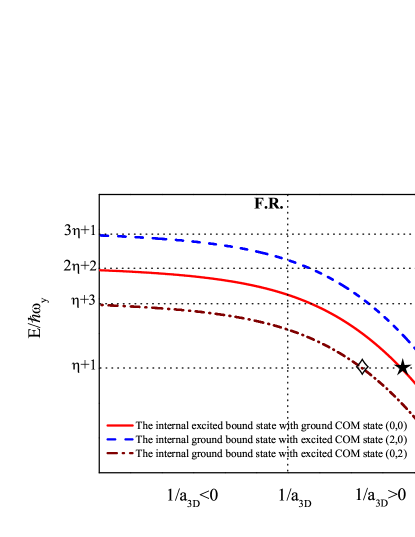
Figure 2: (Color online) Diagram of the confinement induced energy levels in an anisotropic trap or waveguide, with anisotropy $\eta$. The solid line is an internally excited two-particle ground state. The dashed lines correspond to a COM excitations of the two-particle ground state. Confinement induced resonance thresholds occur when these excited molecular states become resonant with two incoming free particles with zero momentum. This is indicated by a star in the internally excited CIR case, which is the only level coupled in the case of a harmonic trap. For anharmonic traps, these additional levels become coupled to input atomic states with zero transverse excitation, and acquire additional anharmonic energy shifts.

IV Anharmonic CIR in a quasi-1D waveguide

While Eq (17) is valid for a relatively deeply bound molecule, it neglects both anharmonic and waveguide corrections to the internal molecular energy $E_{b}$. The question of which transverse molecular quantum numbers $N_{x},$$N_{y}$ are accessible in terms of selection rules also needs to be addressed more carefully. In this section, we therefore treat the general case of a quasi-1D confining waveguide with an asymmetric confining potential. This case can be continuously changed to the limit of the 2D trap, which is treated in more detail in the following section. Due to the small anharmonic parameter $\alpha$, the anharmonic term $H_{a}$ will be treated as a perturbation to $H_{h}$ .

IV.1 Harmonic CIR

Firstly, we consider the anisotropic waveguide without the anharmonic perturbation $H_{a}$. While this has been treated previouslyPeng2010C , we revisit it here as a first step to solving the anharmonic case. The origin of the confinement induced resonance is due to two scattering atoms forming a virtual molecule via their S-wave interaction. The energy of the resulting two atom quasi-bound state in a waveguide is written as:

$$E_{M}^{(0)} = E_{CM}+E_{b}$$ (18)

$$= \left(N_{x}+\frac{1}{2}\right)\hbar\omega_{x}+\left(N_{y}+\frac{1}{2}\right)\hbar\omega_{y}+E_{b}$$

Here $E_{CM}$ is the energy of the COM excitation, $\left(N_{x},N_{y}\right)$ are the quantum numbers of the COM, and $E_{b}$ is the binding energy of the two atoms. This becomes resonant with two incoming atoms near zero momentum when $E_{M}^{(0)}=E_{scatt}$, where $E_{scatt}$ is the incoming free-particle energy. This is trivially given in the zero-momentum, harmonic case by:

$$E_{scatt} = 2E_{A}^{(0)}$$ (19)

$$= \hbar\omega_{x}+\hbar\omega_{y}\,.$$

By solving the eigenproblem of the relative Hamiltonian of the two atoms $H_{h}^{rel}$ , we can obtain the relation between the binding energy $E_{b}$ and the 3D s-wave scattering length $a_{3D}$. This is known from previous work Peng2010C , by solving for the dimensionless energy $\epsilon$ of the molecular ground state, where $\epsilon\equiv E_{b}/\hbar\omega_{y}-\left(\eta+1\right)/2$, as given in Eq (15). We note that, just as with Eq (15) in the previous section, the dimensionless energy $\epsilon$ is defined so that it includes the change in transverse confinement energies. With this definition, $E_{b}$ reduces to the free-space binding energy in the limit of weak confinement or strong binding.

The dimensionless ground state molecular energy $\epsilon$ is given by an implicit equation Peng2010C :

$$\frac{d_{y}}{a_{3D}}=-\frac{1}{\sqrt{\pi}}\mathcal{F}_{1}\left(\epsilon,0\right)\,,$$ (20)

where the RHS is defined by the definite integral

$$\mathcal{F}_{1}\left(\epsilon,0\right)=\int_{0}^{\infty}dt\left[\frac{\sqrt{\eta}\exp\left(\epsilon t/2\right)}{\sqrt{t\left(1-e^{-\eta t}\right)\left(1-e^{-t}\right)}}-\frac{1}{t^{3/2}}\right]\,.$$ (21)

In the strong binding limit, the limiting behavior of this integral is:

$$\lim_{\epsilon\rightarrow-\infty}-\frac{\mathcal{F}_{1}\left(\epsilon,0\right)}{\sqrt{\pi}}=\sqrt{\frac{2\left|E_{b}\right|}{\hbar\omega_{y}}}.$$ (22)

This is leads to the free-space three-dimensional binding energy result, Eq (12), as one expects in this limit. Combining Eq (15) and Eq (18), the threshold condition for a harmonic trap can be summarized compactly in one equation as

$$\epsilon+N_{x}\eta+N_{y}=0\,,$$ (23)

so that:

$$\frac{d_{y}}{a_{3D}}=-\frac{1}{\sqrt{\pi}}\mathcal{F}_{1}\left(-\left[N_{x}\eta+N_{y}\right],0\right)\,.$$ (24)

Further resonances are anticipated if we consider relative atomic motion. Such an internally excited molecular state is described by a completely different integral equation. For the first excited state of the internal motion, one obtains:

$$\frac{d_{y}}{a_{3D}}=-\frac{1}{\sqrt{\pi}}\mathcal{F}_{e}\left(\epsilon_{e},0\right)\,,$$ (25)

where the RHS is now defined by the definite integral

$$\mathcal{F}_{e}\left(\epsilon_{e},0\right) = \int_{0}^{\infty}dt\biggl{[}e^{\epsilon_{e}t/2}\sqrt{\frac{\eta}{t}}\biggl{(}\frac{1}{\sqrt{\left(1-e^{-\eta t}\right)\left(1-e^{-t}\right)}}$$ (26)

$$-1\biggr{)}-\frac{1}{t^{3/2}}\biggr{]}\,.$$

The CIR threshold condition including both internal and COM excitations is therefore

$$\epsilon_{e}+N_{x}\eta+N_{y}=0\,,$$ (27)

so that:

$$\frac{d_{y}}{a_{3D}}=-\frac{1}{\sqrt{\pi}}\mathcal{F}_{e}\left(-\left[N_{x}\eta+N_{y}\right],0\right)\,.$$ (28)

The above equations 23 and 27 give threshold conditions in the limit of small anharmonicity, for coupling to either the internal ground or excited state respectively, with center-of-mass quantum numbers included in the final resonant state.

As such, they give an elegant picture of the possible resonances, including both internal and COM excitations. However, if the anharmonic term $H_{a}$ is not included, the two incoming atoms in a transverse ground state cannot couple to the transverse excited molecular states during the collision. Hence, for harmonic confinement there is only one observable CIR resonance no matter how anisotropic the transverse confinement Peng2010C . This is described by the last equation above, Eq (28), on setting $N_{x}=N_{y}=0$.

In reality, anharmonic terms do occur. These lead both to couplings that allow COM excitations, and to energy shifts which alter the resonance locations. In the following analysis, we will assume that there are only COM excitations, and we will apply perturbation theory to the bound state COM energies predicted by Eq (23).

IV.2 Anisotropic, anharmonic CIR

If the anharmonic perturbation $H_{a}$ is now introduced, the COM motion will be mixed with the relative motion by the anharmonicity of the confining trap. Then the transversely excited COM molecular states can couple to the scattering state of the two incoming atoms in the transverse ground state. However, both the atomic and molecular states now have energy levels shifted by anharmonic corrections. This means that the fundamental resonance equation is modified from Eq (23) for the harmonic trap case. It is now:

$$\epsilon+N_{x}\eta+N_{y}+\epsilon_{a}\left(N_{x},N_{y}\right)=0\,,$$ (29)

where $\epsilon_{a}\left(N_{x},N_{y}\right)$ is the anharmonic correction to the relative energy levels for a COM excitation with quantum numbers $\left(N_{x},N_{y}\right)$. This has been treated already in the deeply bound limit in Eq (17). We now treat this in the general case.

From Eq (8), one must include the input anharmonicity in the atomic levels, which for the case of two atoms in an initial atomic transverse ground state is given by Eq (9). Next, we consider the effects of anharmonicity on the bound or molecular energies.

With a quartic anharmonicity which is symmetric around the origin, there are constraints on the types of coupling that can occur to the COM motion. In particular, with a symmetric input state having $N_{x}=N_{y}=0$, one must have a symmetric resonance state. This implies that only even COM quantum numbers are strongly coupled. There is also a weak coupling to odd COM quantum numbers, caused by cubic anharmonic parameters, which we treat in the next section. The lowest of the strong nonlinear resonances occur when $\left(N_{x},N_{y}\right)=\left(2,0\right)$ or $\left(0,2\right)$. Consequently the resonance splits if the transverse confinement is anisotropic.

We give a detailed calculation of the effects of anharmonic confinement on the bound-state energies of these resonances in the Appendix. Using these results, we arrive at the resonance condition for the $N_{x}=2$ state ,

$$\epsilon+2\eta+\alpha_{x}\eta\left(\frac{27}{32}-\frac{5\eta}{32\epsilon}+\frac{3\eta^{2}}{320\epsilon^{2}}\right)$$

$$+\alpha_{y}\left(\frac{-9}{32}-\frac{1}{32\epsilon}+\frac{3}{320\epsilon^{2}}\right) = 0$$ (30)

In like manner, the resonance condition for the $N_{y}=2$ state is,

$$\epsilon+2+\alpha_{x}\eta\left(\frac{-9}{32}-\frac{\eta}{32\epsilon}+\frac{3\eta^{2}}{320\epsilon^{2}}\right)$$

$$+\alpha_{y}\left(\frac{27}{32}-\frac{5}{32\epsilon}+\frac{3}{320\epsilon^{2}}\right) = 0$$ (31)

These results can be compared with Eq (17), which were obtained in the previous section, dealing with the case of a deeply bound molecular state. On dropping terms scaling with $1/\epsilon$, the two conditions agree in the limit of strong molecular binding, with $\epsilon\rightarrow-\infty$.

For experiments using optical lattices with equal wavelengths in each direction, one finds that:

$$\alpha_{x}\eta=\alpha_{y}\equiv\alpha$$ (32)

Then the resonance conditions can be reduced to a simpler form. For $\left(N_{x},N_{y}\right)=\left(2,0\right)$, one obtains

$$\epsilon+2\eta+\alpha\left(\frac{9}{16}-\frac{5\eta+1}{32\epsilon}+\frac{3\left(\eta^{2}+1\right)}{320\epsilon^{2}}\right)=0\,,$$ (33)

and for $\left(N_{x},N_{y}\right)=\left(0,2\right)$ :

$$\epsilon+2+\alpha\left(\frac{9}{16}-\frac{\eta+5}{32\epsilon}+\frac{3\left(\eta^{2}+1\right)}{320\epsilon^{2}}\right)=0\,.$$ (34)

Solving these equations requires the use of a nonlinear equation solving numerical algorithm, like the Newton-Raphson method which we use in Fig.3 to obtain theoretical results for comparison with experiment.

Now we are ready to understand the dominant effects observed in the recent Innsbruck experimentHaller2010C . The atoms are prepared in a 1D tube geometry using two orthogonal pairs of counter-propagating laser fields to create a trapping environment. In the case of transverse isotropic confinement, due to the small collision energy and large energy interval between the transverse energy levels, only the first excited molecular states $\left(N_{x}=2,N_{y}=0\right)$ and $\left(N_{x}=0,N_{y}=2\right)$ of the COM motion which are degenerate can couple to the scattering state of two incoming atoms. In this isotropic situation, the results of ACIR are similar to those of HCIR and also agree well with the experiment, as long as the anharmonicity of the confinement is not too large. Due to the broad resonances and fitting techniques used, the isotropic experimental data has too little precision to accurately distinguish between ACIR and CIR resonances.

By increasing the transverse anisotropy $\eta=\omega_{x}/\omega_{y}$ , the molecular states $\left(N_{x}=2,N_{y}=0\right)$ and $\left(N_{x}=0,N_{y}=2\right)$ of the COM motion are no longer degenerate. A splitting of the ACIR is expected, which has been observed in the experiment. By contrast, no splitting of the linear HCIR resonance is predicted. Thus, the double resonance observed experimentally is a clear signature of the ACIR resonance. It is also a sign that if there is any internally excited HCIR effect in this experiment, it is relatively suppressed compared to the ACIR effect which involves COM excitations.

The theoretical predictions of the CIRs compared with the experimental results Haller2010C are presented in Fig.3. As we can see, the predictions of the COM-relative coupling theory are consistent with the experimental data.

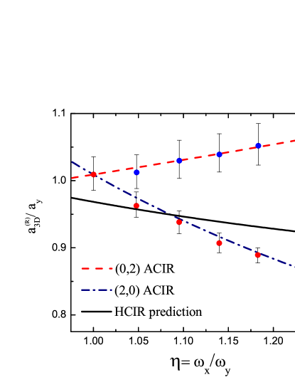
Figure 3: (Color online) The predictions of ACIR resonances using first-order anharmonic perturbation theory comparing with the experimental data Haller2010C . The black solid curve is the result of a generalized Olshanii’s HCIR model Peng2010C . Here the anisotropy $\eta$ is changed by increasing the frequency $\omega_{x}$ with a fixed $\omega_{y}=2\pi\times 13.2(2)$kHz (or $\omega_{1}$ inHaller2010C ), which resulted in an anharmonic parameter of $\alpha=-0.133$ .

In these experiments, the resonances were identified as occurring at the point of maximum molecular loss. This leads to an offset between the apparent and true resonance due to finite resonance widths. To compensate for this in the original experimental publication, the data was fitted to the isotropic HCIR prediction by adding a small constant offset to make it equal to the theoretical results at $\eta=1$. We follow a similar fitting procedure here, for consistency, but we fit the offset to the isotropic ACIR prediction instead. Note that the anharmonic parameter is different to that used in Table 1, because Table 1 gives values representative of a range of experiments, while in each of the figures we use the data from the relevant experiment.

At the point $\eta=1$, there is transversely isotropic confinement, and the ACIR prediction is in accord with the Olshanii CIR, apart from anharmonic corrections. However, as the transverse confinement becomes more and more anisotropic, the internally excited HCIR resonance persists as a single resonance except for a small frequency shift Peng2010C . Both ACIR theory and experiment show a clear splitting of the original resonance with increasing trap asymmetry. There is excellent quantitative agreement in the amount of splitting. In these experiments, there is strong evidence for the COM excited ACIR resonances.

IV.3 Multiple resonance ACIR at large anisotropy

As the transverse anisotropy $\eta$ becomes even larger, the energy spacing in the $y$ direction decreases, and more transversely excited molecular states can readily couple to the initial scattering state. Consequently, more additional COM resonances can occur. By contrast, there is still only one internal HCIR resonance predicted no matter how large the transverse anisotropy. However, several multiple resonances are observed experimentally at large anisotropy. In order to understand these, we now consider the other transverse states.

As in the previous section, given any coupling parameter ($a_{3D}$), the unperturbed binding energy $\epsilon$ is determined by Eq (20), which as an implicit equation involving the integral $\mathcal{F}_{1}\left(\epsilon,0\right)$. We then use perturbation theory to calculate the dimensionless anharmonic energy shift $\epsilon_{a}$. Hence, we obtain the ACIR resonance position of $a_{3D}$ for arbitrary odd and even COM quantum numbers from the solutions to the overall resonance equation, Eq (29).

For brevity, we will refer to an arbitrary molecular COM resonance as simply $\left(N_{x},N_{y}\right)$. The general form of the resulting anharmonic shifts is derived in the Appendix, for arbitrary quartic anharmonic parameters. We include both odd and even order resonances, because, as remarked earlier, there are both cubic and quartic anharmonic couplings, which leads to the possibility of both even and odd ACIR resonances. However, for simplicity we do not include the relatively small cubic energy shifts.

For comparison to current experiments, we are interested in the case of equal optical trapping wavelengths, which means that $\alpha_{x}\eta=\alpha_{y}\equiv\alpha$. From the Appendix, the general form of the resulting anharmonic shifts for resonances corresponding to the $\left(N_{x},N_{y}\right)$ COM state is as follows,

$$\epsilon_{a}\left(N_{x},N_{y}\right)/\alpha=\frac{3(N_{y}^{2}+N_{y}+N_{x}^{2}+N_{x})-9}{16}-\\ -\frac{2N_{y}+1+\eta(2N_{x}+1)}{32\epsilon}+\frac{3\left(\eta^{2}+1\right)}{320\epsilon^{2}}$$ (35)

This allows the positions of ACIR denoted by $a_{3D}$ to be calculated. In the experimental reports of multiple resonances at large anisotropy (Fig.4 Haller2010C ), the loss rates are plotted as a function of magnetic field, rather than $a_{3D}$. We therefore make use of the relation between the 3D scattering length $a_{3D}$ and $B$-field for the relevant ${}^{137}Cs$ Feshbach resonance Lange2009D , which is,

$$\frac{a_{3D}}{a_{bg}}=\frac{B-18.1}{B+11.1}\cdot\frac{B-47.944}{B-47.78}\cdot\frac{B-53.457}{B-53.449}$$ (36)

and,

$$\frac{a_{3D}}{a_{bg}} = \frac{1}{1875a_{0}}\sqrt{\frac{\hbar\eta}{m\omega_{x}}}\cdot\frac{a_{3D}}{a_{y}}$$ (37)

$$= 0.681\sqrt{\eta}\cdot\frac{a_{3D}}{a_{y}}$$

Hence, the predicted magnetic field at resonance can be calculated. In order to compare our theory to these experiments, the regime of anisotropy $\eta$ considered is $\left[1.4,2.3\right]$ . We also note that in these experiments, the trapping frequency $\omega_{y}$ is varied, so the effective anharmonicity parameter $\alpha$ therefore changes at different anisotropy.

Then main results are summarized in Fig.4, which compares theory to experiment. The experimental resonance points are obtained from the raw data as the start of the resonance edges, which is appropriate for this type of resonance experiment. No fitting parameters or shifts are employed. Since error bars were not given in the experimental plot, we are unable to estimate these.

Most observed resonances can be easily identified, which are coded in the same color as the corresponding theoretical predictions. There are $25$ identified resonances, all of which are in excellent agreement with theoretical calculations. However, there are $5$ smaller resonances not identified, which are indicated by the empty triangles.

Apart from experimental issues, possible explanations for these unidentified peaks are:

• Higher-order many-body ACIR resonances. Combination 4-body cluster resonances could occur at intermediate points between the identified 2-body resonances. For example, the three unidentified resonances between $(0,1)$ and $(0,2)$ could be caused by the simultaneous excitation of $(0,1)$ and $(0,2)$ in a 4-body collision. Similarly, the three resonances we have identified as $(1,1)$ resonances could also be caused by 4-body excitation of $(0,3)$ and $(0,4)$ ACIR resonances.

• Anharmonically shifted internal HCIR resonances. We have not calculated these, as the anharmonic shifts of these resonances are outside the scope of this paper. However, this mechanism provides a possible explanation for the two unidentified resonances between $(0,4)$ and $(2,0)$.

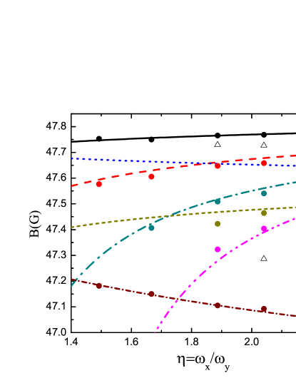
Figure 4: (Color online) The resonant magnetic field $B$ vs anisotropy $\eta$ at ACIR resonances (solid and dotted lines identified alongside the figure) from first-order anharmonic perturbation theory comparing with the Innsbruck experiment data (round circles). Data is extracted from multiple resonance scans Haller2010C at absorption edges. Here the anisotropy $\eta$ is changed by decreasing the frequency $\omega_{y}$ with a fixed $\omega_{x}=2\pi\times 16.6(2)$kHz which results in an $\eta$-dependent anharmonic parameter $\alpha=-0.106\eta$ .

V Anharmonic CIR in a quasi-2D system

For a quasi-2D system, atoms are tightly confined in the axial direction, and can freely move in two transverse directions. In the following section, we will derive the anharmonic CIR resonance properties in this case as well. As we will show, these results can be also obtained from results in the previous section by taking one of the confinement frequencies to zero. However, the direct calculation given here is an important check on the consistency of our approach. In the case of an optical lattice, the trapping potential is of form:

$$U^{ext}\left(\mathbf{r}\right) = V_{z}\cos^{2}\left(\frac{2\pi z}{\lambda}\right)$$

$$\approx \frac{1}{2}m\omega^{2}z^{2}\left(1+\frac{\alpha z^{2}}{d^{2}}\right)$$

Here, $V_{z}$ is the potential well-depth with one standing-wave trapping laser at optical wavelength $\lambda$ . This leads to the trap frequency $\omega$ in the $z$ direction. We note that cubic anharmonic terms are also possible due to focusing effects in this case also.

As before, we use a scale length of the reduced oscillator length $d=\sqrt{2\hbar/m\omega}$ , and define a single atom oscillator length $a_{\perp}=\sqrt{\hbar/m\omega}$, and a small anharmonic parameter $\alpha$, so that for an optical lattice,

$$\alpha=\frac{-8\pi^{2}\hbar}{3\lambda^{2}m\omega}\,.$$ (39)

The Hamiltonian of two atoms in a quasi-2D system is then,

$$H=H_{1}+H_{2}+U\left(\mathbf{r}_{1}-\mathbf{r}_{2}\right)\,,$$ (40)

where,

$$H_{i}=-\frac{\hbar^{2}}{2m}\nabla_{\mathbf{r}_{i}}^{2}+\frac{1}{2}m\omega^{2}z_{i}^{2}\left(1+\alpha\frac{z_{i}^{2}}{d^{2}}\right)\qquad\left(i=1,2\right)\,.$$ (41)

As previously, $U\left(\mathbf{r}_{1}-\mathbf{r}_{2}\right)$ is the interatomic interaction, and we set

$$\mathbf{R} = \frac{1}{2}\left(\mathbf{r}_{1}+\mathbf{r}_{2}\right)$$

$$\mathbf{r} = \mathbf{r}_{1}-\mathbf{r}_{2}\,.$$ (42)

Then Eq.(40) becomes,

$$H=H_{h}+H_{a}$$ (43)

Where,

$$H_{h} = \left(-\frac{\hbar^{2}}{2M}\nabla_{\mathbf{R}}^{2}+\frac{1}{2}M\omega^{2}Z^{2}\right)+$$ (44)

$$+\left[-\frac{\hbar^{2}}{2\mu}\nabla_{\mathbf{r}}^{2}+\frac{1}{2}\mu\omega^{2}z^{2}+V\left(\mathbf{r}\right)\right]$$

$$= H_{h}^{CM}+H_{h}^{rel}$$

$$H_{a} = \alpha\cdot\frac{m\omega^{2}}{2d^{2}}\left(2Z^{4}+3Z^{2}z^{2}+\frac{1}{8}z^{4}\right)$$ (45)

Here $\mathbf{r}=\left(x,y,z\right)$ , $\mathbf{R}=\left(X,Y,Z\right)$ , and $M=2m$ , $\mu=m/2$ .

Due to the small anharmonic parameter $\alpha$ , the anharmonic term $H_{a}$ can be treated as a perturbation to $H_{h}$ . Firstly, consider the case without the small perturbation $H_{a}$ . An anharmonic confinement-induced resonance is expected when the energy of the virtual molecule is degenerate with the energy of two incoming atoms from the axial ground state,

$$E_{M}^{(0)}=E_{CM}+E_{b}=E_{scatt}$$ (46)

Where $E_{CM}=\left(N+\frac{1}{2}\right)\hbar\omega$, $E_{scatt}=\hbar\omega$, and the binding energy $E_{b}$ is determined by,

$$\frac{d}{a_{3D}}=-\frac{1}{\sqrt{\pi}}\mathcal{F}_{2}\left(\epsilon,0\right)$$ (47)

and the integral expression required here is given by,

$$\mathcal{F}_{2}\left(\epsilon,0\right)=\int_{0}^{\infty}dt\left[\frac{\exp\left(\frac{1}{2}\epsilon t\right)}{t\sqrt{1-e^{-t}}}-\frac{1}{t^{3/2}}\right]$$ (48)

We define $E_{b}=\left(\epsilon+1/2\right)\hbar\omega$ , $d=\sqrt{\hbar/\mu\omega}$ . The lowest resonance occurs as $N=2$; however, this is not coupled to the incoming states unless there is an anharmonic term in the potential.

If the anharmonic term $H_{a}$ is included, we need to consider how the energy of the input atomic states and virtual molecule $E_{M}$ is affected by this perturbation.

V.1 The anharmonic energy $E_{M}^{(1)}$

Including the first order modification $E_{M}^{(1)}$ , we arrive at the following integral equation for $\epsilon$,

$$\left(N+\frac{1}{2}\right)\hbar\omega+\left(\epsilon+\frac{1}{2}\right)\hbar\omega+E_{M}^{(1)}\left(\epsilon\right)=\hbar\omega+\frac{3}{8}\alpha\hbar\omega$$ (49)

By solving this equation, the binding energy $\epsilon^{(R)}$ at the resonance is obtained. Then substituting $\epsilon^{(R)}$ into the Eq.(47), we will obtain the 3D scattering length $a_{3D}^{(R)}$ at the resonance. Following the general procedure outlined in the Appendix, we find that a resonance occurs at:

$$N+\epsilon+\frac{\alpha}{32}\left[6N\left(N+1\right)-9-\frac{\left(2N+1\right)}{\epsilon}+\frac{3}{10\epsilon^{2}}\right]=0$$ (50)

Hence, we obtain the equation that $\epsilon$ should satisfy for states with $N=2$ ,

$$\epsilon+2+\alpha\left(\frac{27}{32}-\frac{5}{32\epsilon}+\frac{3}{320\epsilon^{2}}\right)=0$$ (51)

This result is identical to Eq (31) in the limit of $\eta\rightarrow 0$, as one might expect, since the quasi-1D trap becomes two-dimensional in this limit. However, it is instructive that one cannot regain this limit directly from Eq (34), which holds for optical lattices with equal wavelengths. The reason is very simple: in an optical lattice at low transverse confinement frequency, the transverse wave-function becomes more and more deconfined. This increases the relative anharmonicity, as given in Eq (4), so that $\alpha\sim 1/\omega$. Therefore, our anharmonic perturbation theory would break down for a weakly confined 1D system described by Eq (34). Optical lattices that are only weakly confining require a full Bloch wave-function theory, typically requiring detailed numerical diagonalization Buchler .

From Eq.(51), we can calculate the relative binding energy $\epsilon$ for the states of $N=2$, in the two-dimensional limit. Then, substituting into Eq (47), the corresponding resonance scattering length $a_{3D}^{(R)}$ is obtained. Here, in order to calculate $\epsilon$ numerically, we use the Newton-Raphson method as before, together with a numerical calculation of $\mathcal{F}_{2}\left(\epsilon,0\right)$. The position of the ACIR denoted by the 3D scattering length as a function of the anharmonic parameter $\alpha d^{2}$ is presented in Fig.5, and we can see that the 2D ACIR is predicted at the regime of $a_{3D}>0$ . This is in contrast to the internal HCIR resonance, which occurs for the attractive regime with $a_{3D}<0$.

Now we can compare these predictions with 2D resonances observed in the recent Innsbruck experimentHaller2010C . When one of the lattice lasers is turned off, the system approaches a 2D geometry. All resonances disappear except one at $a_{3D}>0$ . Given the average anharmonicity in this experiment of $\alpha=-0.121$, we expect as shown in Fig.5 to find a resonance at

$$a_{3D}=0.85a_{\perp}$$ (52)

The observed resonances occur at a constant ratio between $a_{3D}$ and $a_{\perp}$, such that

$$\frac{a_{3D}}{a_{\perp}}a_{3D}=0.84(3)$$ (53)

This is consistent with the prediction of 2D ACIR. The anharmonicity $\alpha$ in the experiments was varied through a small range as the trapping frequency varied, and we have calculated the ratio at the average anharmonicity.

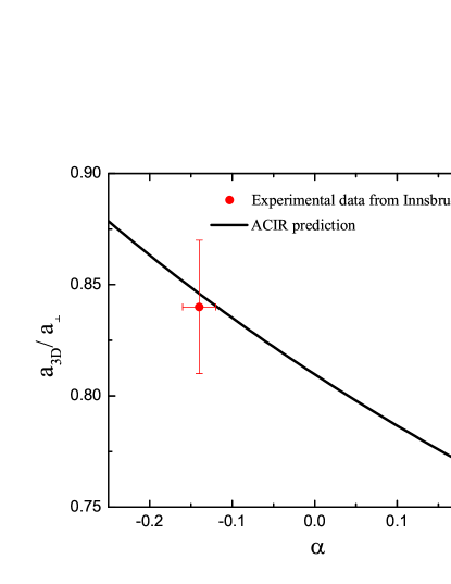
Figure 5: (Color online) Predicted resonance positions of 2D CIRs, as a function of the dimensionless anharmonic parameter $\alpha$. The experimental data point is an average from experiments Haller2010C , plotted at the average anharmonicity value.

Finally, we plot the predicted variation of $a_{3D}^{(R)}$ with transverse confinement parameter $a_{\perp}$, at a fixed value of $\omega\alpha$ corresponding to the Innsbruck experiments, in Fig.6. This data is also in excellent quantitative agreement with ACIR predicted resonance positions.

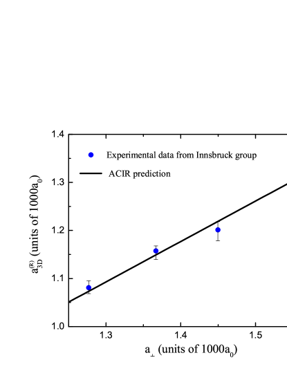
Figure 6: (Color online) Predicted resonance positions of 2D ACIR resonances, as a function of the transverse confinement parameter, $a_{\perp}$. The experimental data points are taken from experiment Haller2010C , where circles indicate resonances identified by absorption edges.

In anharmonic trap experiments, we would generically expect both the ACIR resonance at $a_{3D}>0$, and the internal HCIR resonance at $a_{3D}<0$ to be observed. The Innsbruck experiments Haller2010C show clear evidence for the ACIR resonance, but not the internal HCIR resonance. The Cambridge experiments Frohlich2010R have shown evidence for HCIR resonances, although the magnetic field scans were not large enough to observe any ACIR resonances. The question of which is observed will depend on the size of the anharmonic parameter, the dynamics of the experiment, and the method of detection of the resonance. It appears likely that the molecular loss technique is particularly sensitive to COM resonances.

VI conclusion

We have extended the theory of the harmonic confinement-induced resonance to include the effects of anharmonic confinement, or ACIR, since previous harmonic theories cannot explain phenomena observed in recent experiments. In the presence of anharmonic perturbation of the confinement trap, the COM motion of two atoms couples to the relative motion, and additional resonances appear. We have calculated the energy of the resulting new resonances up to first order in perturbation theory. The results agree well with experiments, with both even and odd order multiple resonances being found. These differences are not just small perturbations on previous HCIR predictions, and show large qualitative differences from the predictions for harmonic traps.

ACIR resonances due to COM excitations are always present in Feshbach systems with any form of transverse confinement. The important issue is that for harmonic traps the Kohn theorem prevents these resonances from being coupled to incoming atoms in the two-body sector of the COM ground state. However, experimental optical traps do have relatively large anharmonic parameters, which allows the resonances due to COM motion to be coupled to incoming scattering states. We find excellent quantitative agreement between ACIR predictions and recent experimental observations of confinement resonances, both in one and two dimensional traps.

*

Appendix A Anharmonic Perturbation Theory

We consider how the relative anharmonic energy of the virtual molecule $\epsilon_{a}$ Eq.(29), is calculated from the anharmonic perturbation $H_{a}$, including the effects of anharmonicity on both relative and COM motion. For space reasons, we do not give all the overlap integrals, as the calculations are similar in all cases. Instead, we focus on the most important cases.

First, note that the dimensionless change in the relative anharmonic perturbation energy is:

$$\epsilon_{a}=\frac{1}{\hbar\omega_{y}}\left[E_{M}^{(1)}-2E_{A}^{(1)}\right]\,,$$ (54)

where $E_{A}^{(1)}$ is the perturbed atomic anharmonic energy given in Eq (8), and $E_{M}^{(1)}$ is the first order perturbation theory correction to the energy of the virtual molecule:

$$E_{M}^{(1)} = \left\langle\Psi_{N_{x}N_{y}}\psi_{b}\right|H_{a}\left|\psi_{b}\Psi_{N_{x}N_{y}}\right\rangle\,.$$ (55)

Here, $\left|\Psi_{N_{x}N_{y}}\psi_{b}\right\rangle=\left|\Psi_{N_{x}N_{{}_{y}}}\right\rangle\left|\psi_{b}\right\rangle$ is the eigenstate of $H_{h}$. This is treated as the zero-order wave-function, and includes both relative and COM motion. Next, we introduce $\left|\Psi_{N_{x}N_{{}_{y}}}\right\rangle$ as the unperturbed wave-function of the COM Hamiltonian, so that

$$\left|\Psi_{N_{x}N_{y}}\right\rangle=\left|\phi_{N_{x}}\right\rangle\left|\phi_{N_{y}}\right\rangle$$ (56)

with the standard two-dimensional harmonic oscillator solution of:

$$\left|\phi_{N_{x,y}}\right\rangle=\frac{\exp\left(-2\xi_{x,y}^{2}\right)H_{N_{x,y}}\left(2\xi_{x,y}\right)}{\sqrt{\pi^{1/2}d_{x,y}2^{N_{x,y}-1}N_{x,y}!}}$$ (57)

where $\xi_{i}=\left(X/d_{x},Y/d_{y}\right)$. We now turn to the task of evaluating $E_{M}^{(1)}$, the anharmonic correction to the total molecular energy at a given unperturbed dimensionless energy $\epsilon$.

A.1 The relative wave-function $\left|\psi_{b}\right\rangle$

The specific form of $\left|\psi_{b}\right\rangle$ can be obtained by directly solving the eigenproblem of $H_{h}^{rel}$ ,

$$\left[-\frac{\hbar^{2}}{2\mu}\nabla_{\mathbf{r}}^{2}+\frac{1}{2}\mu\omega_{x}^{2}x^{2}+\frac{1}{2}\mu\omega_{y}^{2}y^{2}+V\left(\mathbf{r}\right)\right]\left|\psi\right\rangle=E\left|\psi\right\rangle$$ (58)

The wave-function $\left|\psi\right\rangle$ can be written as,

$$\left|\psi\right\rangle = \psi_{0}\left(\mathbf{r}\right)-\int_{0}^{\infty}d\mathbf{r}^{\prime}G_{E}\left(\mathbf{r},\mathbf{r}^{\prime}\right)V\left(\mathbf{r}^{\prime}\right)\psi\left(\mathbf{r}^{\prime}\right)$$ (59)

$$= \psi_{0}\left(\mathbf{r}\right)-\mathcal{R}\cdot\frac{2\pi\hbar^{2}a_{3D}}{\mu}G_{E}\left(\mathbf{r},0\right)$$

Where $\psi_{0}\left(\mathbf{r}\right)$ is the regular solution of Eq.(58) and,

$$\mathcal{R}=\left[\frac{\partial}{\partial r}r\psi\left(\mathbf{r}\right)\right]_{r=0}$$ (60)

Here, we have use the pseudo-potential approximation. For a bound state, the solution of Eq.(58) $\left|\psi\right\rangle$ should vanish as $r\rightarrow\infty$, hence $\psi_{0}\left(\mathbf{r}\right)=0$ . Then the constant $\mathcal{R}$ is only a normalization coefficient. The Green’s function $G_{E}\left(\mathbf{r},\mathbf{r}^{\prime}\right)$ is the solution of the following equation,

$$\left[-\frac{\hbar^{2}}{2\mu}\nabla_{\mathbf{r}}^{2}+\frac{1}{2}\mu\omega_{x}^{2}x^{2}+\frac{1}{2}\mu\omega_{y}^{2}y^{2}-E\right]G_{E}\left(\mathbf{r},\mathbf{r}^{\prime}\right)=\delta\left(\mathbf{r}-\mathbf{r}^{\prime}\right)$$ (61)

The form of the Green’s function $G_{E}\left(\mathbf{r},0\right)$ for a bound state can be easily calculated,

$$G_{\epsilon<0}\left(\mathbf{r},0\right) = \frac{\sqrt{\eta}I_{1}\left(\mathbf{r}\right)}{2\pi^{3/2}d^{3}\hbar\omega_{y}}\exp\left(-\frac{\eta x^{2}+y^{2}}{2d^{2}}\right)$$ (62)

where we introduce the integral representation:

$$I_{1}\left(\mathbf{r}\right)=\int_{0}^{\infty}dt\frac{\exp\left(\frac{\epsilon}{2}t-\frac{1}{t}\frac{z^{2}}{d^{2}}-\frac{e^{-\eta t}}{1-e^{-\eta t}}\frac{\eta x^{2}}{d^{2}}-\frac{e^{-t}}{1-e^{-t}}\frac{y^{2}}{d^{2}}\right)}{\sqrt{t\left(1-e^{-\eta t}\right)\left(1-e^{-t}\right)}}$$ (63)

Recalling that $\eta=\omega_{x}/\omega_{y}$ , and $E=\left(\epsilon+\eta/2+1/2\right)\hbar\omega_{y}$, the bound-state wave-function is,

$$\left|\psi_{b}\right\rangle = \mathcal{N}\exp\left(-\frac{\eta x^{2}+y^{2}}{2d^{2}}\right)I\left(\mathbf{r}\right)\,,$$ (64)

where $\mathcal{N}$ is the normalization coefficient.

A.2 1D COM overlap terms

We can now calculate the overlap integrals which give the anharmonic contributions to the quasi-1D and quasi-2D ACIR resonances. In order to calculate the first order modification $E_{M}^{(1)}$ , we focus on the $\left(N_{x},N_{y}\right)$ COM state. The relevant terms are: $\left\langle\Psi_{N_{x}N_{y}}\right|X^{4}\left|\Psi_{N_{x}N_{y}}\right\rangle$ , $\left\langle\Psi_{N_{x}N_{y}}\right|Y^{4}\left|\Psi_{N_{x}N_{y}}\right\rangle$ , $\left\langle\Psi_{N_{x}N_{y}}\right|X^{2}\left|\Psi_{N_{x}N_{y}}\right\rangle$ , $\left\langle\Psi_{N_{x}N_{y}}\right|Y^{2}\left|\Psi_{N_{x}N_{y}}\right\rangle$.

We define $D_{x,y}=\sqrt{\hbar/2m\omega_{x,y}}=d_{x,y}/2$ as the transverse confinement parameter of an atom pair in the following calculation. Hence:

$$\left\langle\psi_{N_{x}N_{y}}\right|X^{4}\left|\psi_{N_{x}N_{y}}\right\rangle = \frac{1}{\sqrt{\pi}D_{x}2^{N_{x}}N_{x}!}\int_{-\infty}^{\infty}X^{4}\exp\left(-\frac{X^{2}}{D_{x}^{2}}\right)\left[H_{N_{x}}\left(\frac{X}{D_{x}}\right)\right]^{2}dX$$ (65)

$$= \frac{1}{\sqrt{\pi}D_{x}2^{N_{x}}N_{x}!}\cdot D_{x}^{5}\sqrt{\pi}2^{N_{x}}N_{x}!\left[\left(N_{x}+\frac{1}{2}\right)\left(N_{x}+\frac{3}{2}\right)+\frac{1}{2}N_{x}\left(N_{x}-1\right)\right]$$

$$= \left[\left(N_{x}+\frac{1}{2}\right)\left(N_{x}+\frac{3}{2}\right)+\frac{1}{2}N_{x}\left(N_{x}-1\right)\right]D_{x}^{4}$$

$$\left\langle\psi_{N_{x}N_{y}}\right|X^{2}\left|\psi_{N_{x}N_{y}}\right\rangle = \frac{1}{\sqrt{\pi}D_{x}2^{N_{x}}N_{x}!}\int_{-\infty}^{\infty}X^{2}\exp\left(-\frac{X^{2}}{D_{x}^{2}}\right)\left[H_{N_{x}}\left(\frac{X}{D_{x}}\right)\right]^{2}dX$$ (66)

$$= \frac{1}{\sqrt{\pi}D_{x}2^{N_{x}}N_{x}!}\cdot D_{x}^{3}\sqrt{\pi}2^{N_{x}}N_{x}!\left(N_{x}+\frac{1}{2}\right)$$

$$= \left(N_{x}+\frac{1}{2}\right)D_{x}^{2}$$

By using the exchange symmetry of $x$ and $y$ , we can easily obtain,

$$\left\langle\psi_{N_{x}N_{y}}\right|Y^{4}\left|\psi_{N_{x}N_{y}}\right\rangle=\left[\left(N_{y}+\frac{1}{2}\right)\left(N_{y}+\frac{3}{2}\right)+\frac{1}{2}N_{y}\left(N_{y}-1\right)\right]D_{y}^{4}$$ (67)

$$\left\langle\psi_{N_{x}N_{y}}\right|Y^{2}\left|\psi_{N_{x}N_{y}}\right\rangle=\left(N_{y}+\frac{1}{2}\right)D_{y}^{2}$$ (68)

Here, we have used the formulas,

$$\int_{-\infty}^{\infty}dtt^{2}e^{-t^{2}}H_{n}^{2}\left(t\right)=\sqrt{\pi}2^{n}n!\left(n+\frac{1}{2}\right)$$ (69)

$$\int_{-\infty}^{\infty}dtt^{4}e^{-t^{2}}H_{n}^{2}\left(t\right)=\sqrt{\pi}2^{n}n!\left[\left(n+\frac{1}{2}\right)\left(n+\frac{3}{2}\right)+\frac{1}{2}n\left(n-1\right)\right]$$ (70)

A.3 1D Internal motion overlap terms

The relevant terms are now: $\left\langle\psi_{b}\right|x^{4}\left|\psi_{b}\right\rangle$ , $\left\langle\psi_{b}\right|y^{4}\left|\psi_{b}\right\rangle$, $\left\langle\psi_{b}\right|x^{2}\left|\psi_{b}\right\rangle$ , $\left\langle\psi_{b}\right|y^{2}\left|\psi_{b}\right\rangle$. For the bound state of the relative motion $\left|\psi_{b}\right\rangle$ , the main contribution of the integrals, e.g., $\left\langle\psi_{b}\right|x^{4}\left|\psi_{b}\right\rangle$ etc., comes from the regime around the origin. We note that the energy parameter $\epsilon$ is negative. The form of $\left|\psi_{b}\right\rangle$ near the origin $r=0$ can be easily obtained from Eq.(64),

$$\left|\psi_{b}\right\rangle \approx \left(\frac{-\epsilon}{2}\right)^{1/4}\frac{1}{\sqrt{\pi d_{y}}}\cdot\frac{\exp\left(-\sqrt{-2\epsilon}r/d_{y}\right)}{r}$$ (71)

which has been normalized. Then,

$$\left\langle\psi_{b}\right|x^{2}\left|\psi_{b}\right\rangle = \frac{1}{\pi d_{y}}\sqrt{\frac{-\epsilon}{2}}\int_{0}^{2\pi}\int_{0}^{\pi}\int_{0}^{\infty}r^{2}\sin^{3}\theta\cos^{2}\phi\exp\left(-\frac{2\sqrt{-2\epsilon}r}{d_{y}}\right)drd\theta d\phi$$ (72)

$$= -\frac{d_{y}^{2}}{12\epsilon}$$

$$\left\langle\psi_{b}\right|x^{4}\left|\psi_{b}\right\rangle = \frac{1}{\pi d_{y}}\sqrt{\frac{-\epsilon}{2}}\int_{0}^{2\pi}\int_{0}^{\pi}\int_{0}^{\infty}r^{4}\sin^{4}\theta\cos^{4}\phi\frac{\exp\left(-2\sqrt{-2\epsilon}r/d_{y}\right)}{r^{2}}r^{2}\sin\theta drd\theta d\phi$$ (73)

$$= \frac{3d_{y}^{4}}{40\epsilon^{2}}$$

$$\left\langle\psi_{b}\right|y^{2}\left|\psi_{b}\right\rangle = \frac{1}{\pi d_{y}}\sqrt{\frac{-\epsilon}{2}}\int_{0}^{2\pi}\int_{0}^{\pi}\int_{0}^{\infty}r^{2}\sin^{2}\theta\sin^{2}\phi\frac{\exp\left(-2\sqrt{-2\epsilon}r/d_{y}\right)}{r^{2}}r^{2}\sin\theta drd\theta d\phi$$ (74)

$$= -\frac{d_{y}^{2}}{12\epsilon}$$

$$\left\langle\psi_{b}\right|y^{4}\left|\psi_{b}\right\rangle = \frac{1}{\pi d_{y}}\sqrt{\frac{-\epsilon}{2}}\int_{0}^{2\pi}\int_{0}^{\pi}\int_{0}^{\infty}r^{4}\sin^{4}\theta\sin^{4}\phi\frac{\exp\left(-2\sqrt{-2\epsilon}r/d_{y}\right)}{r^{2}}r^{2}\sin\theta drd\theta d\phi$$ (75)

$$= \frac{3d_{y}^{4}}{40\epsilon^{2}}$$

A.4 The first order modification of the energy $E_{M}^{(1)}$

Using the overlap integral results given above, we find that:

$$\left\langle\psi_{N_{x}N_{y}}\psi_{b}\right|H_{a}^{x}\left|\psi_{N_{x}N_{y}}\psi_{b}\right\rangle=\frac{\alpha_{x}\hbar\omega_{x}}{32}\left[6N_{x}\left(N_{x}+1\right)+3-\frac{\eta\left(2N_{x}+1\right)}{\epsilon}+\frac{3\eta^{2}}{10\epsilon^{2}}\right]$$ (76)

$$\left\langle\psi_{N_{x}N_{y}}\psi_{b}\right|H_{a}^{y}\left|\psi_{N_{x}N_{y}}\psi_{b}\right\rangle=\frac{\alpha_{y}\hbar\omega_{y}}{32}\left[6N_{y}\left(N_{y}+1\right)+3-\frac{\left(2N_{y}+1\right)}{\epsilon}+\frac{3}{10\epsilon^{2}}\right]$$ (77)

Combining this with the atomic energy correction gives the overall result for an equal wavelength 1D optical lattice, in which $\alpha_{x}\omega_{x}=\alpha_{y}\omega_{y}$ :

$$\epsilon_{a}^{(1D)}=\frac{\alpha}{32}\left[6(N_{y}^{2}+N_{y}+N_{x}^{2}+N_{x})-18-\frac{\eta\left(2N_{x}+1\right)+\left(2N_{y}+1\right)}{\epsilon}+\frac{3\left(\eta^{2}+1\right)}{10\epsilon^{2}}\right]$$ (78)

Following similar procedures, from Eq 77, the anharmonic correction in the corresponding 2D case leads to:

$$\epsilon_{a}^{(2D)}=\frac{\alpha}{32}\left[6N\left(N+1\right)-9-\frac{\left(2N+1\right)}{\epsilon}+\frac{3}{10\epsilon^{2}}\right]$$ (79)

.

References

- (1) M. D. Girardeau, J. Math. Phys. 1, 516 (1960); Phys. Rev. 139, B500 (1965).
- (2) E. H. Lieb and W. Liniger, Phys. Rev. 130, 1605 (1963); E. H. Lieb, ibid, 130, 1616 (1963).
- (3) C. N. Yang, C. P. Yang, J. Math. Phys. 10, 1115 (1969).
- (4) D. M. Gangardt and G. V. Shlyapnikov, Phys. Rev. Lett. 90, 010401 (2003).
- (5) K. V. Kheruntsyan, D. M. Gangardt, P. D. Drummond, and G. V. Shlyapnikov, Phys. Rev. Lett. 91, 040403 (2003); K. V. Kheruntsyan, D. M. Gangardt, P. D. Drummond, and G. V. Shlyapnikov, Phys. Rev. A 71, 053615 (2005).
- (6) B. Laburthe Tolra, K. M. O’Hara, J. H. Huckans, W. D. Phillips, S. L. Rolston, and J. V. Porto, Phys. Rev. Lett. 92, 190401 (2004).
- (7) T. Kinoshita, T. R. Wenger and D. S. Weiss, Science 305, 1125 (2004).
- (8) E. Haller, M. Gustavsson, M. J. Mark, J. G. Danzl, R. Hart, G. Pupillo, and H. C. Nagerl, Science 325, 1224 (2009).
- (9) Berezins.Vl, Soviet Physics Jetp-Ussr 32, 493 (1971).
- (10) J. M. Kosterlitz and D. J. Thouless, Journal of Physics C-Solid State Physics 6, 1181 (1973).
- (11) Z. Hadzibabic, P. Kruger, M. Cheneau, B. Battelier, and J. Dalibard, Nature 441, 1118 (2006).
- (12) H. Feshbach, Annals of Physics 281, 519 (1962).
- (13) T. Kohler, K. Goral, and P. S. Julienne, Rev. Mod. Phys. 78, 1311 (2006).
- (14) I. Bloch, J. Dalibard, and W. Zwerger, Rev. Mod. Phys. 80, 885 (2008).
- (15) M. Olshanii, Phys. Rev. Lett. 81, 938 (1998).
- (16) T. Bergeman, M. G. Moore, and M. Olshanii, Phys. Rev. Lett. 91, 163201 (2003).
- (17) Y. Nishida, and S. Tan, Physical Review Letters 101, 170401 (2008); Y. Nishida, and S. Tan, Physical Review A 82, 062713 (2010).
- (18) G. Lamporesi, J. Catani, G. Barontini, Y. Nishida, M. Inguscio, and F. Minardi, Phys. Rev. Lett. 104, 153202 (2010).
- (19) S.-G. Peng, S. S. Bohloul, X.-J. Liu, H. Hu, and P. D. Drummond, Phys. Rev. A 82, 063633 (2010).
- (20) D. S. Petrov, M. Holzmann, and G. V. Shlyapnikov, Phys. Rev. Lett. 84, 2551 (2000).
- (21) D. S. Petrov and G. V. Shlyapnikov, Phys. Rev. A 64, 012706 (2001).
- (22) P. Naidon, E. Tiesinga, W. F. Mitchell, and P. S. Julienne, New Journal of Physics 9, 19 (2007).
- (23) E. Haller, M. J. Mark, R. Hart, J. G. Danzl, L. Reichsollner, V. Melezhik, P. Schmelcher, and H.-C. Nagerl, Phys. Rev. Lett. 104, 153203 (2010). Note that in comparisons with this paper, we use the notation , .
- (24) Bernd Frohlich, Michael Feld, Enrico Vogt, Marco Koschorreck, Wilhelm Zwerger, and Michael Kohl, Phys. Rev. Lett. 106, 105301 (2011).
- (25) C. Vale, private communication.
- (26) W. Kohn, Phys. Rev. 123, 1242 (1961); J. F. Dobson, Phys. Rev. Lett. 73, 2244 (1994).
- (27) V. Peano, M. Thorwart, C. Mora and R. Egger, New J. Phys. 7, 192 (2005).
- (28) J. P. Kestner and L. M. Duan, New J. Phys. 12, 11 (2010).
- (29) Simon Sala, Philipp-Immanuel Schneider, Alejandro Saenz, arXiv:1104.1561 (2011).
- (30) P. D. Drummond, K. V. Kheruntsyan, H. He, J Opt B 1, 387-395 (1999); K. V. Kheruntsyan and P. D. Drummond, Phys. Rev. A 61, 063816 (2000); P. D. Drummond and K. V. Kheruntsyan, Phys. Rev. A 70, 033609 (2004).
- (31) A. D. Lange, K. Pilch, A. Prantner, F. Ferlaino, B. Engeser, H. C. Nagerl, R. Grimm, and C. Chin, Phys. Rev. A 79, 013622 (2009).
- (32) Hans Peter Büchler, Phys. Rev. Lett. 104, 090402 (2010).