Proton fraction in the inner neutron-star crust

Abstract

Monte Carlo simulations of neutron-rich matter of relevance to the inner neutron-star crust are performed for a system of $A\!=\!5,000$ nucleons. To determine the proton fraction in the inner crust, numerical simulations are carried out for a variety of densities and proton fractions. We conclude—as others have before us using different techniques—that the proton fraction in the inner stellar crust is very small. Given that the purported “nuclear pasta” phase in stellar crusts develops as a consequence of the long-range Coulomb interaction among protons, we question whether pasta formation is possible in such proton-poor environments. To answer this question, we search for physical observables sensitive to the transition between spherical nuclei and exotic pasta structures. Of particular relevance is the static structure factor $S(k)$—an observable sensitive to density fluctuations. However, no dramatic behavior was observed in $S(k)$. We regard the identification of physical observables sensitive to the existence—or lack-thereof—of a pasta phase in proton-poor environments as an open problem of critical importance.

I Introduction

Neutron stars are unique laboratories for the study of matter under extreme conditions of density and isospin asymmetry Weber (1999); Glendenning (2000). Indeed, the conditions in the interior of neutron stars are so extreme that they are unattainable in terrestrial laboratories. Thus, neutron stars—and the exotic phases within—owe their existence to the presence of enormous gravitational fields. To maintain hydrostatic equilibrium throughout the star, these enormous gravitational fields must be balanced by the pressure support of its underlying constituents. This results in an enormous dynamic range of pressures and densities that enables one to probe the equation of state (EOS) far away from the equilibrium density of normal nuclei Piekarewicz (2009).

Neutron stars contain a non-uniform crust above the uniform liquid mantle (or stellar core). The core is comprised of a uniform assembly of neutrons, protons, electrons, and muons packed to densities that may exceed that of normal nuclei by up to an order of magnitude. The highest density attained in the core depends critically on the equation of state of neutron-rich matter which at those high densities is presently poorly constrained. The core accounts for almost all of the mass and most of the size of the neutron star. However, at densities of about half of normal nuclear density, the uniform core becomes unstable against cluster formation. At these “low” densities the average inter-nucleon separation increases to such an extent that it becomes energetically favorable for the system to segregate into regions of normal density (nuclear clusters) and regions of low density (dilute neutron vapor). Such a clustering instability signals the transition from the uniform liquid core to the non-uniform crust. Note, however, that the precise value of the crust-to-core transition density is presently unknown, as it is sensitive to the poorly constrained density dependence of the symmetry energy Horowitz and Piekarewicz (2001).

The solid crust is divided into an outer and an inner region. In particular, the outer crust spans a region of about seven orders of magnitude in density (from about $10^{4}{\rm g/cm^{3}}$ to $4\times 10^{11}{\rm g/cm^{3}}$ Baym et al. (1971); Ruester et al. (2006); Roca-Maza and Piekarewicz (2008)). Structurally, the outer crust is comprised of a Coulomb lattice of neutron-rich nuclei embedded in a uniform electron gas. As the density increases—and given that the electronic Fermi energy increases rapidly with density—it becomes energetically favorable for electrons to capture into protons. This results in the formation of Coulomb crystals of progressively more neutron-rich nuclei. Eventually, the neutron-proton asymmetry becomes too large for the nuclei to absorb any more neutrons and the excess neutrons go into the formation of a dilute neutron vapor; this signals the transition from the outer to the inner crust.

In this contribution we are interested in modeling the structure of the inner crust. The outer-to-inner crust transition density is predicted to occur at about $4\times 10^{11}{\rm g/cm^{3}}$ Baym et al. (1971); Ruester et al. (2006); Roca-Maza and Piekarewicz (2008). At this—neutron-drip—density the neutron-rich nucleus (¹¹⁸Kr) that comprises the crystalline lattice is unable to retain any more neutrons. Thus, the top layer of the inner crust consists of a Coulomb crystal of neutron-rich nuclei immersed in a uniform electron gas and a dilute—likely superfluid—neutron vapor. In contrast, at the bottom layer of the inner crust the density has become high enough (of the order of $10^{14}{\rm g/cm^{3}}$) to “melt” the crystal into a uniform mixture of neutrons, protons, and electrons. Yet the transition from the highly-ordered crystal to the uniform liquid is both interesting and complex. This is because distance scales that were well separated in both the crystalline phase (where the long-range Coulomb interaction dominates) and in the uniform phase (where the short-range strong interaction dominates) become comparable. This unique situation gives rise to “Coulomb frustration”. Frustration, a phenomenon characterized by the existence of a very large number of low-energy configurations, emerges from the impossibility to simultaneously minimize all “elementary” interactions in the system. Whereas protons are correlated at short distances by attractive strong interactions, they are anti-correlated at large distances because of the Coulomb repulsion. Whenever these short and large distance scales are well separated (as in the outer crust) protons bind into nuclei that are then segregated in a crystal lattice. However, as these length scales become comparable—at densities of about $10^{13}\!-\!10^{14}$ g/cm³ as in the inner crust—competition among the elementary interactions results in the formation of complex topological structures collectively referred to as “nuclear pasta”. Given that these complex structures are very close in energy, it has been speculated that the transition from the highly ordered crystal of spherical nuclei to the uniform phase must proceed through a series of changes in the dimensionality and topology of these structures Ravenhall et al. (1983); Hashimoto et al. (1984). Moreover, due to the preponderance of low-energy states, frustrated systems display an interesting and unique low-energy dynamics.

Interestingly enough, a seemingly unrelated condensed-matter problem—the strongly-correlated electron gas—appears to be connected to the nuclear pasta. In the case of the electron gas, one aims to characterize the transition from the low-density Wigner crystal (where the Coulomb potential dominates) to the uniform high-density Fermi liquid (where the kinetic energy dominates) Fetter and Walecka (1971). It has been argued that instead of the expected first order phase transition, the transition is mediated by the emergence of “microemulsions”, namely, exotic (“pasta-like”) structures. Indeed, it has been shown that in two-spatial dimensions first-order phase transitions are forbidden in the presence of long-range (e.g., Coulomb) forces Jamei et al. (2005). One should note that no generalization of this theorem to three dimensions exists. Hence, although the existence of pasta phases in both core-collapse supernovae and neutron stars may be plausible Ravenhall et al. (1983); Hashimoto et al. (1984), there is no guarantee that they exist. Actually, in a recent publication Oyamatsu and Iida have shown that pasta formation may not be universal and that its existence (or lack-thereof) is intimately related to the density dependence of the symmetry energy Oyamatsu and Iida (2007). In particular, the authors concluded that pasta formation requires models with a soft symmetry energy, namely, ones that increase slowly with density.

Although the complex dynamics of the electron gas may shed light on the possible emergence of pasta phases in the stellar crust, an essential difference between these two systems remains. Whereas the constituents of the electron gas (i.e., electrons) are all electrically charged and thus experience long-range forces, the neutrons in the crust interact solely via short-range forces. Thus, a large neutron fraction in the inner crust could hinder the formation of the nuclear pasta. Indeed, pure neutron matter does not cluster. So given that the proton fraction in the crust is highly sensitive to the density dependence of the symmetry energy, the emergence of pasta phases involves a delicate interplay between: (i) the symmetry energy (which controls the proton fraction), (ii) the surface tension (which favors spherical nuclei), and (iii) the Coulomb interaction (which favors deformation). It is this interesting and unique problem that we propose to study here via numerical simulations.

Monte-Carlo simulations will be performed directly in terms of the nucleon constituents. Although we have already performed simulations of this kind Horowitz et al. (2004a, b); Horowitz et al. (2005), in the present manuscript we aim to improve them in two critical areas. First, in our previous work a screened Coulomb interaction between the protons was assumed with a screening length fixed at $10$ fm. Although it was argued that no major qualitative changes are expected from such an approximation, in this contribution we evaluate the Coulomb interaction exactly via an Ewald summation. For completeness, an appendix has been included where a detailed derivation of the Ewald summation is presented for a system of protons embedded in a uniform electron gas. Second, our earlier simulations were all performed at the single proton fraction of $Y_{p}\!=\!0.2$. This value was chosen as it is intermediate between the large values attained in core-collapse supernovae and the low proton fractions characteristic of the inner crust of cold—fully catalyzed—neutron stars. Instead, in this work we will simulate neutron-rich matter for a variety of densities and proton fractions, albeit for a relatively small number of nucleons ($A\!=\!5,000$). In this way, the optimum proton fraction will be determined by imposing $\beta$-equilibrium.

We should note that for the large proton fractions characteristic of core-collapse supernovae ($Y_{p}\!=\!0.3$–$0.5$) there appears to be agreement that the transition from the ordered Coulomb crystal to the uniform phase must proceed via intermediate pasta phases (such as rods, slabs, tubes, etc.). This agreement has been reached whether one uses numerical simulations Horowitz et al. (2004a, b); Horowitz et al. (2005); Watanabe et al. (2003, 2005, 2009) or mean-field approximations with a variety of effective interactions Maruyama et al. (2005); Avancini et al. (2008, 2009); Newton and Stone (2009); Shen et al. (2011). What is unclear, however, is whether such exotic pasta shapes will still develop in the proton-poor environment of the inner stellar crust. For example, mean-field models that impose $\beta$-equilibrium predict proton fractions at densities of relevance to the inner crust of only a few percent Maruyama et al. (2005); Avancini et al. (2008, 2009); Shen et al. (2011). To our knowledge, no numerical simulations have been carried out with proton fractions less than $Y_{p}\!=\!0.1$ Watanabe et al. (2003). Thus, our manuscript revolves around the following three fundamental questions: (a) Do numerical simulations support the very low proton fractions predicted by mean-field calculations? (b) Does the transition from a highly-ordered crystal of spherical nuclei to a uniform Fermi liquid must proceed via intermediate pasta phases even when the proton fraction is very small? (c) Can one identify a set of robust physical observables that are sensitive to the formation of the nuclear pasta?

We have organized the manuscript as follows. In Sec. II we introduce the model and develop the formalism necessary to carry out the Monte-Carlo simulations. Results are presented in Sec. III for the potential energy as a function of density and proton fraction. The optimal proton fraction is then determined by minimizing the total energy per nucleon of the system. The pair-correlation function (for both protons and neutrons) and the corresponding static-structure factor are computed with the aim of identifying sensitive observables to the formation of the nuclear pasta. Our conclusions and suggestions for future work are presented in Sec. IV.

II Formalism

We start this section by reviewing the semi-classical model that while simple, contains the essential physics of “Coulomb frustration”, namely, competing interactions consisting of a short-range nuclear attraction and a long-range Coulomb repulsion Horowitz et al. (2004a). We stress that the long-range Coulomb interaction among the protons represents the critical ingredient for pasta formation. Hence the importance of establishing whether the proton fraction in the inner stellar crust is large enough to help (or hinder) the formation of the exotic pasta structures. A variety of static observables will be computed using Monte-Carlo simulations having neutrons, protons, and electrons as the main constituents. As the system is simulated directly in terms of its basic constituents, there is no need to assume a-priori any specific nuclear shape, such as rods, slabs, tubes, etc.

The total potential energy of the system includes both short-range nuclear and long-range Coulomb contributions. That is,

$$V({\bf r}_{1},\ldots,{\bf r}_{A})=V_{\rm Nucl}({\bf r}_{1},\ldots,{\bf r}_{A})+V_{\rm Coul}({\bf r}_{1},\ldots,{\bf r}_{A})\;.$$ (1)

The nuclear potential is assumed to consist of a sum of “elementary” two-body interactions of the following form:

$$V_{\rm Nucl}({\bf r}_{1},\ldots,{\bf r}_{A})=\sum_{i<j=1}^{A}v_{{}_{NN}}(r_{ij})=\sum_{i<j=1}^{A}\Big{[}ae^{-r_{ij}^{2}/\Lambda}+\Big{(}b+c\,\tau_{i}\tau_{j}\Big{)}e^{-r_{ij}^{2}/2\Lambda}\Big{]}\;,$$ (2)

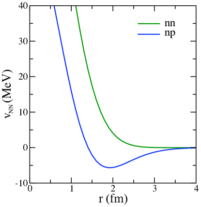
where the inter-particle distance has been denoted by $r_{ij}\!\equiv\!|{\bf r}_{i}\!-\!{\bf r}_{j}|$ and the isospin of the nucleon as $\tau$—with $\tau\!=\!1$ for a proton and $\tau\!=\!-\!1$ for a neutron. The model parameters ($a$, $b$, $c$, and $\Lambda$) were calibrated in Ref. Horowitz et al. (2004a) and are given by the following values: $a\!=\!110$ MeV, $b\!=\!-26$ MeV, $c\!=\!24$ MeV, and $\Lambda\!=\!1.25~{}{\rm fm}^{2}$. Although not accurately calibrated, this set of parameters were fitted to several ground-state properties Horowitz et al. (2004a). In particular, Monte Carlo simulations using this simple interaction are able to account for the saturation of symmetric nuclear matter while precluding the binding of pure neutron matter at all densities Horowitz et al. (2004a). Note, however, that given that such classical simulations are unable to reproduce the momentum distribution of a quantum Fermi gas, the effective $NN$ interaction must be properly adjusted to compensate for this shortcoming. In particular—unlike a realistic neutron-neutron ($nn$) interaction that is attractive at intermediate distances— the effective $nn$ interaction adopted here is (essentially) repulsive at all distances; see Fig. 1.

Figure 1: (Color online) Nucleon-nucleon potential employed in our semi-classical simulations Horowitz et al. (2004a).

For the Coulomb interaction we assume that the protons are immersed in a uniform neutralizing electron background. Note that at the densities of relevance to the stellar crust, the electrons behave to a good approximation as a non-interacting free Fermi gas. For such a system the Coulomb energy may be written in terms of the electrostatic potential as follows:

$$V_{Coul}({\bf r}_{1},\ldots,{\bf r}_{Z})=\frac{1}{2}e\sum_{i=1}^{Z}\Phi({\bf r}_{i})-\frac{eZ}{2V}\int_{V}\Phi({\bf r})d^{3}r\;.$$ (3)

Here $Z$ is the number of protons (and neutralizing electrons), $V$ is the simulation volume, and the electrostatic potential $\Phi({\bf r})$ satisfies Poisson’s equation. Given that numerical simulations must involve a finite number of particles, we rely on periodic boundary conditions in an attempt to minimize finite-size effects. For the case of the short-range nuclear interaction, the implementation of the minimum image convention is both simple and accurate: a given particle in the system interacts only with the closest image of all remaining particles Allen and Tildesley (1987); Frenkel and Smit (1996); Vesely (2001). Indeed, the short-range character of the $NN$ force guarantees that the interactions with all images that are farther away will be exponentially suppressed. This prescription, however, is not valid for the long-range Coulomb potential. In this case a given particle in $V$ interacts not only will all remaining particles in the simulation volume but, in addition, with all periodic images. As such, the source of the electrostatic potential $\Phi({\bf r})$ in Poisson’s equation consists of all protons in the simulation volume $V$, all their periodic images, and the uniform electron background. That is,

$$\rho({\bf r})=e\sum_{i=1}^{Z}\sum_{{\bf n}}\delta\Big{(}{\bf r}-({\bf r}_{i}-{\bf n}L)\Big{)}-e\frac{Z}{V}\;,$$ (4)

where ${\bf n}=(n_{x},n_{y},n_{z})$ is a triplet of integers and $L\!\equiv\!V^{1/3}$.

A method that computes accurately and efficiently the Coulomb potential is based on the (90 year old!) Ewald summation Ewald (1921). The basic idea behind the Ewald sum is to add and subtract $Z$ individual smeared charges at the exact location of each (point) proton. The role of each negative charge is to screen the corresponding (point) proton charge over a distance of the order of the smearing parameter $a$. As long as $a$ is significantly smaller than the box length $L$, the resulting (screened) two-body potential will become short ranged and thus amenable to be treated using the minimum-image convention. What remains then is a periodic system of smeared positive charges together with the neutralizing electron background. In configuration space this remaining long-range contribution is slowly convergent. The great merit of the Ewald sum is that the long-range contribution can be made to converge rapidly if evaluated in momentum space, i.e., as a Fourier sum. Indeed, the Fourier sum is rapidly convergent because momentum (${\bf k}$) modes satisfying $|{\bf k}|a\!\gg\!1$ make a negligible contribution to the sum. Hence, by suitably tuning the value of the smearing parameter $a$, the evaluation of the Coulomb potential may be written in terms of two rapidly convergent sums; one in configuration space and one in momentum space. The derivation and implementation of the Ewald sum is now part of the standard literature Allen and Tildesley (1987); Frenkel and Smit (1996); Toukmaji and Board (1996); Vesely (2001). Yet, for both convenience and completeness, we have provided in the appendix a detailed derivation of the Ewald formula for a system of $Z$ protons immersed in a neutralizing and uniform electron background. Here we only summarize the essential results.

Assuming $Z$ protons confined to a simulation volume $V\!=\!L^{3}$ and immersed in a uniform neutralizing electron background, the Coulomb potential may be written in the following form:

$$V_{\rm Coul}({\bf r}_{1},\ldots,{\bf r}_{Z})=\left(\frac{e^{2}}{L}\right)U_{\rm Coul}({\bf s}_{1},\ldots,{\bf s}_{Z})\;.$$ (5)

This structure reveals that the Coulomb potential is an interaction with no intrinsic scale. That is, once a dimensionful parameter has been identified—$v_{0}\!\equiv\!e^{2}/L$ in the present case—the dimensionless Coulomb potential $U$ depends exclusively on the scaled coordinates ${\bf s}_{i}\!\equiv\!{\bf r}_{i}/L$. As mentioned above, the Ewald construction relies on the introduction of an artificial smearing parameter $a$ that naturally divides the Coulomb potential into two contributions: a short-range contribution that converges rapidly in configuration space and a long-range one that converges rapidly in momentum space. That is,

$$U_{\rm Coul}({\bf s}_{1},\ldots,{\bf s}_{Z})=\frac{1}{2}\sum_{i\neq j}\Big{[}u_{\rm sr}({\bf s}_{ij})+u_{\rm lr}({\bf s}_{ij})\Big{]}+U_{0}\;.$$ (6)

Here the—two-body—short- and long-range contributions are given by

$$u_{\rm sr}({\bf s}) =\frac{{\rm erfc}(s/s_{0})}{s}\;,$$ (7a)

$$u_{\rm lr}({\bf s}) =\sum_{{\bf l}\neq 0}w(l)\exp(-2\pi i{\bf l}\cdot{\bf s})=\sum_{{\bf l}\neq 0}\frac{\exp(-\pi^{2}s_{0}^{2}\,l^{2})}{\pi l^{2}}\exp(-2\pi i{\bf l}\cdot{\bf s})\;,$$ (7b)

where $s_{0}\!\equiv\!a/L$ is the dimensionless smearing parameter and $U_{0}$ is an overall constant:

$$U_{0}=\frac{Z}{2}u_{\rm lr}(0)-\frac{Z}{\sqrt{\pi}s_{0}}-\frac{\pi s_{0}^{2}Z^{2}}{2}\;.$$ (8)

The short-range contribution [Eq. (7a)] represents a (gaussianly) screened two-body Coulomb potential. Indeed, the characteristic $1/s$ fall-off of the Coulomb potential is modified by the complement of the error function which falls rapidly to zero for inter-particle separations significantly larger than the screening length $s_{0}$. The long-range contribution to the Coulomb potential is customarily written in momentum space as a sum that involves the square of the charge form factor times a suitably modified Coulomb propagator in momentum space [see Eq. (36)]. Rapid convergence of the momentum sum is also achieved through the introduction of the smearing parameter [see Eq. (7b)]. However, the evaluation of the momentum sum often remains the most numerically demanding part of the computation, so various efficient methods have been designed for the purpose of expediting the Fourier sum Frenkel and Smit (1996). In our case we will settle for a relatively simple approach that ultimately leads to the form of $u_{\rm lr}({\bf s})$ given above (see appendix). Not surprisingly, this form also involves a numerically demanding Fourier sum. Yet, the advantage of the present method is that $u_{\rm lr}({\bf s})$ may be precomputed in a fine mesh before the start of the simulation. Hence, during the actual simulation the evaluation of $u_{\rm lr}({\bf s})$ is implemented via a look-up table and a simple interpolation scheme Toukmaji and Board (1996). This approach results in significant savings in processing time with little compromise in accuracy. In the present contribution we have selected a smearing parameter that is significantly smaller than the box length, namely, $s_{0}\!=\!0.12$.

III Results

In this section we present results for the potential energy per nucleon as a function of density and proton fraction as obtained from our Monte Carlo simulations. In an effort to simulate the quantum-mechanical zero-point motion of the particles, the simulations were carried out at a fixed temperature of $T\!=\!1$ MeV Horowitz et al. (2004a, b); Horowitz et al. (2005). Moreover, in all simulations the number of baryons was fixed at $A\!=\!5,000$ with the proton fraction varying from $Y_{p}\!=\!0$ to $Y_{p}\!=\!0.25$; this is contrast to our earlier simulations that assumed a fixed value of $Y_{p}\!=\!0.2$. Having fixed the number of baryons, the proton fraction, the temperature, and the density of the system, a Metropolis algorithm was used to generate a total of 3,000 Monte Carlo sweeps—with each sweep consisting of $A\!=\!5,000$ particle moves. The first 2,500 sweeps were used to thermalize the system and the last 500 to compute various physical observables. This was done “off-line” by first saving the coordinates of all $5,000$ particles to file (for each of the final 500 sweeps) and then using a post-processor to compute the observables. We focus initially on the energy per particle as a function of density and proton fraction as we aim to estimate whether the proton fraction in the bottom layers of the inner stellar crust is small enough to hinder the formation of the pasta.

Figure 2: (Color online) Monte-Carlo results for the total (nuclear-plus-Coulomb) potential energy of a system of $A\!=\!5,000$ nucleons as a function of density and proton fraction.

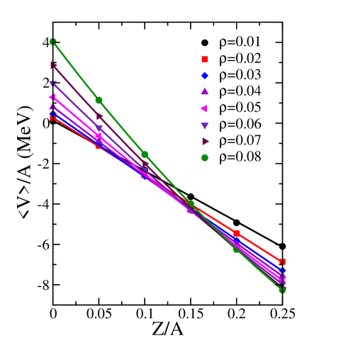
The potential energy per nucleon $\langle V\rangle/A$ as a function of density and proton fraction $y$ is displayed in Fig. 2. (Note that we have used the symbol “$y$” to denote an arbitrary value for the proton fraction; we reserve the symbol “$Y_{p}$” to denote the value obtained from applying the condition of $\beta$-equilibrium). The strong-nuclear interaction favors symmetric $N\!=\!Z$ (i.e., $y\!=\!1/2$) clusters so $\langle V\rangle$ is a monotonically decreasing function of $y$ (at least until $y\!\simeq\!1/2$). The $y\!=\!0$ values are related to the equation of state of pure neutron matter and display the density dependence predicted by the present model. To enforce $\beta$-equilibrium it is convenient—as well as accurate—to fit the $y$ dependence of the potential to a quadratic form. That is,

$$\frac{\langle V\rangle(\rho,y)}{A}=v_{0}(\rho)+v_{1}(\rho)y+v_{2}(\rho)y^{2}\;.$$ (9)

The best-fit values obtained for the three coefficients are displayed in Table 1.

$\rho({\rm fm}^{-3})$	$v_{0}$(MeV)	$v_{1}$(MeV)	$v_{2}$(MeV)
0.010	0.1221	-24.8220	-0.7801
0.020	0.2675	-28.3990	-0.8496
0.030	0.4923	-31.5810	1.3126
0.040	0.8103	-34.7880	5.0355
0.050	1.2924	-39.2340	11.6480
0.060	1.9713	-44.9300	20.6400
0.070	2.8642	-51.6810	30.5050
0.080	4.0295	-60.0800	43.6780

Table 1: Quadratic fit to the $y$-dependence of $\langle V\rangle/A$ as given in Eq. (9).

To determine the optimal proton fraction we compute the total energy per nucleon of the system ($E/A$) as a function of both density and proton fraction $y$. The optimal proton fraction ($Y_{p}$) is then obtained by minimizing $E/A$ with respect to $y$ at fixed density. We write the energy per nucleon of the system in the following form:

$$\frac{E}{A}-m_{n}=-y\Delta m+\frac{T_{n}}{A}+y\frac{(T_{p}+T_{e})}{Z}+\frac{\langle V\rangle}{A}\approx\frac{T_{n}}{A}+y\frac{T_{e}}{Z}+\frac{\langle V\rangle}{A}\;.$$ (10)

Here $\Delta m\!\equiv\!m_{n}\!-\!m_{p}\!-\!m_{e}$ is the neutron-proton-electron mass difference and $T_{n}$, $T_{p}$, and $T_{e}$ represent the kinetic energy of the three constituents. In the above equation the “approximate” sign has been used to indicate that the contribution from $\Delta m$ is negligible (see Fig. 4) and that the electronic kinetic energy $T_{e}$—assumed to be that of a relativistic electron gas—is much larger than the classical proton contribution ($3yT/2$). Note that the energy (kinetic plus rest mass) per particle of a relativistic Fermi gas of particles of mass $m$ and number density $\rho\!=\!k_{\rm F}^{3}/3\pi^{2}$ may be expressed in terms of the dimensionless Fermi momentum $x_{\rm F}\!\equiv\!k_{\rm F}/m$ (and $y_{\rm F}\!\equiv\!\sqrt{1+x_{\rm F}^{2}}$) in the following compact form:

$${\varepsilon}_{{}_{\rm FG}}(x_{\rm F})=\frac{3m}{8}\left[\frac{x_{\rm F}y_{\rm F}(x_{\rm F}^{2}+y_{\rm F}^{2})-\ln(x_{\rm F}+y_{\rm F})}{x_{\rm F}^{3}}\right]=\begin{cases}\displaystyle{m+\frac{3k_{\rm F}^{2}}{10m}+\ldots}&\text{if $k_{\rm F}\!\ll\!m$,}\\ &\\ \displaystyle{\frac{3}{4}k_{\rm F}+\frac{3m^{2}}{4k_{\rm F}}+\ldots}&\text{if $m\!\ll\!k_{\rm F}$.}\end{cases}$$ (11)

Figure 3: (Color online) Two snapshots from a Monte Carlo simulation for a system of $A\!=\!4,000$ nucleons at a baryon density of $\rho\!=\!0.01~{}{\rm fm}^{-3}$ (upper panel) and $\rho\!=\!0.025~{}{\rm fm}^{-3}$ (lower panel). In both cases a proton fraction of $Z/A\!=\!0.2$ and a temperature of $T\!=\!1$ MeV were used Piekarewicz (2009).

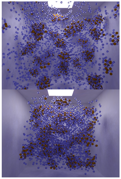
Unfortunately, the neutron contribution $T_{n}$ to the energy of the system is difficult to estimate. This is because at the densities of relevance to the inner crust, the neutrons are either part of the heavy clusters or part of the dilute neutron vapor. (See Fig. 3 for a snapshot of a Monte Carlo simulation that clearly illustrates this scenario.) Presumably, the neutrons bound to the heavy clusters are “sluggish” and thus may be treated classically. The “free” neutrons on the other hand, should probably be modeled as a quantum Fermi gas. However, deciding what fraction of the neutrons are bound to clusters and what fraction remains in the vapor is clearly a model-dependent question. Still, we can make some progress in setting reasonable limits for the proton fraction because the electronic Fermi energy dominates the kinetic energy of the system. To set a lower limit we assume no contribution to the kinetic energy from the neutron vapor. Conversely, a suitable upper limit for the proton fraction is obtained by assuming that all neutrons contribute to the kinetic energy.

Figure 4: (Color online) Enforcing beta equilibrium at a density of $\rho\!=\!0.05~{}{\rm fm}^{-3}$. The various contributions to the energy per nucleon are explained in the text.

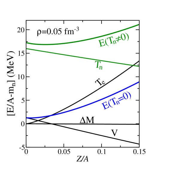
We illustrate how this process is implemented in Fig. 4 where the various contributions to the energy per nucleon have been plotted as a function of the proton fraction for a fixed density of $\rho\!=\!0.05~{}{\rm fm}^{-3}$. As alluded earlier, the contribution from the mass difference $\Delta m$ is negligible. Hence, in the limit of no contribution from the neutron vapor, the proton fraction emerges from a competition between the potential energy—which favors symmetric matter—and the electronic Fermi energy—which favors pure neutron matter. Given that the electronic Fermi energy changes more rapidly with proton fraction than $\langle V\rangle$, $\beta$-equilibrium is reached for the very small value of $Y_{p}\!\simeq\!0.006$. As expected, adding the vapor contribution (as a free Fermi gas of $N$ neutrons) increases the proton fraction by almost a factor of 4; to $Y_{p}\!\simeq\!0.025$. Still, in both cases the proton fraction is very small and significantly smaller—by almost a factor of 10—than the $0.2$ value employed in our earlier simulations Horowitz et al. (2004a, b); Horowitz et al. (2005).

Figure 5: (Color online) Proton fraction computed under the assumption that either all the neutrons are bound into heavy clusters $(N_{\rm vapor}=0)$ or all the neutrons contribute to the Fermi gas energy $(N_{\rm vapor}\!=\!N)$ (see text for details). Also shown is a relativistic mean-field prediction for the proton fraction as described in Ref. Shen et al. (2011).

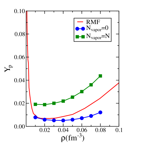
Having implemented the above procedure at all densities, we display in Fig. 5 the predicted proton fraction as a function of baryon density. Our results suggest very low proton fractions over the entire range of densities explored in this work. This finding appears consistent with predictions made using vastly different approaches Maruyama et al. (2005); Avancini et al. (2008, 2009); Shen et al. (2011). For example, in Fig. 5 results are also shown using the relativistic mean-field (RMF) model of Ref. Shen et al. (2011). The precipitous decline in the proton fraction displayed in the figure is driven by the rapid increase with density of the electronic contribution. That is, at the densities of relevance to the inner crust, electron capture is favored because the dilute neutron vapor contributes little to the energy whereas the electrons contribute a lot. This represents robust physics that should be fairly model independent. Thus, we must conclude that the proton fraction in $\beta$-stable, neutron-star matter must be very small at the densities of relevance to pasta formation. Motivated by this finding, we find imperative to determine whether pasta formation can occur in the proton-poor environment of the inner stellar crust. To do so, one must be able to identify observables that are particularly sensitive to the formation of these exotic structures. For reasons that will soon become clear, we focus on the static structure factor.

A fundamental physical observable that contains all information about the excitations of the many-body system is the dynamic response function $S({\bf k},\omega)$. The dynamic response function—which is proportional to the scattering cross section—represents the probability that the system be excited by a probe (e.g., electron, neutrino, etc.) that transfers momentum ${\bf k}$ and energy $\omega$ into the system. To obtain dynamical information of this kind one most resort to Molecular Dynamics simulations—which we hope to carry out in the near future. Unfortunately, Monte Carlo simulations such as the ones implemented here can only reveal static properties. Yet the static structure factor $S({\bf k})$—obtained by integrating the dynamic response over $\omega$—provides a particularly useful (static) observable that is associated with the mean-square density fluctuations in the ground state Fetter and Walecka (1971). Moreover, $S({\bf k})$ is intimately related to a quantity that can be readily determined in computer simulations: the pair-correlation function $g({\bf r})$. Indeed, $S({\bf k})$ and $g({\bf r})$ are simply Fourier transforms of each other. That is Vesely (2001),

$$S({\bf k})=1+\frac{N}{V}\int d^{3}r\Big{(}g({\bf r})-1\Big{)}{\Large{e}}^{-i{\bf k}\cdot{\bf r}}\;.$$ (12)

The pair-correlation function $g({\bf r})$ represents the probability of finding a pair of particles separated by a distance ${\bf r}$. For a uniform fluid containing $N$ particles and confined to a simulation volume $V$, $g(r)$ (which is only a function of the magnitude of ${\bf r}$) may be computed exclusively in terms of the instantaneous positions of the particles. That is,

$$g(r)=1+\frac{V}{4\pi r^{2}N^{2}}\Big{\langle}\sum_{i\neq j}\delta(r-|{\bf r}_{i}-{\bf r}_{j}|)\Big{\rangle}\;,$$ (13)

where the “brackets” represent an ensemble average. Whereas for a uniform fluid the one-body density is constant, interesting two-body correlations emerge as a consequence of the inter-particle dynamics and/or quantum statistics. For example, the characteristic short-range repulsion of the $NN$ interaction precludes particles from approaching each other. This results in a pair-correlation function that vanishes at short separations (see Fig. 6).

Given that the static structure factor accounts for the mean-square density fluctuations in the ground state, it becomes a particularly useful indicator of the critical behavior associated with phase transitions—which themselves are characterized by the development of large (i.e., macroscopic) fluctuations. Indeed, the spectacular phenomenon of “critical opalescence” in fluids is the macroscopic manifestation of abnormally large density fluctuations—and thus abnormally large light scattering—near a phase transition Pathria (1996). In this regard, the static structure factor at zero-momentum transfer provides a unique connection to the thermodynamics of the system Pathria (1996). That is,

$$S({\bf k}\!=\!0)=1+\frac{N}{V}\int d^{3}r\Big{(}g({\bf r})-1\Big{)}=\frac{\langle N^{2}\rangle-\langle N\rangle^{2}}{\langle N\rangle}=\frac{k_{B}T}{\langle N\rangle}\left(\frac{\partial\langle N\rangle}{\partial\mu}\right)_{T,V}=\rho k_{B}T\kappa_{T}\;,$$ (14)

where $k_{B}$ is Boltzmann’s constant, $\mu$ is the chemical potential, and $\kappa_{T}$ is the isothermal compressibility of the system. The isothermal compressibility $\kappa_{T}$ is reminiscent of the specific heat which accounts for energy, rather than density, fluctuations. They both play a fundamental role in identifying the onset of critical phenomena.

Figure 6: (Color online) Pair correlation function $g(r)$ and static structure factor $S(k)$ for protons (left panels) and neutrons (right panels) for a variety of proton fractions at a fixed baryon density of $\rho\!=\!0.03~{}{\rm fm}^{-3}$.

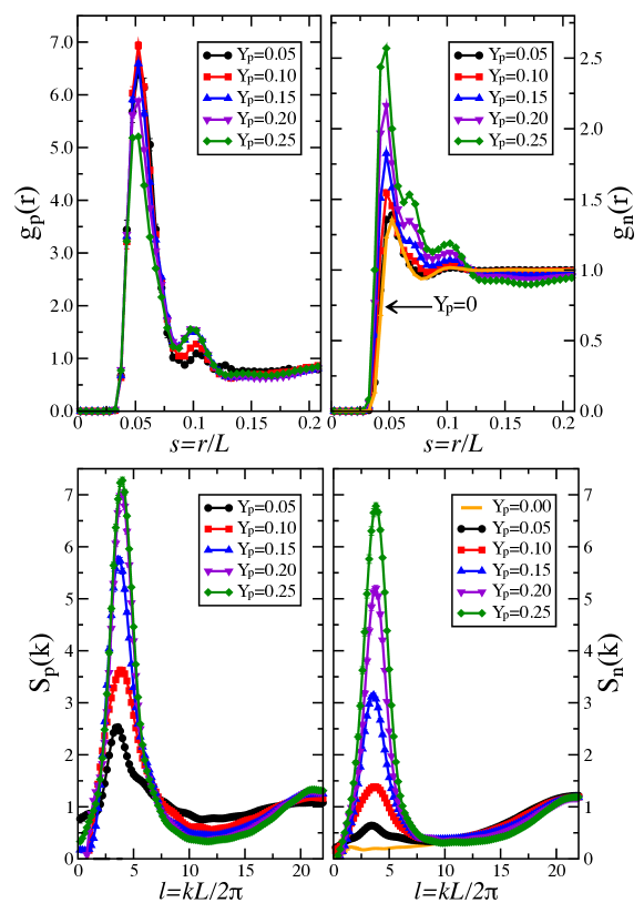
We conclude this section by displaying in Fig. 6 the pair correlation function $g(r)$ (upper panels) and static structure factor $S(k)$ (lower panels) for both protons (left panels) and neutrons (right panels) at the fixed density of $\rho\!=\!0.03~{}{\rm fm}^{-3}$. At this value of the density pasta structures are known to be present—at least for moderately large proton fractions (see Fig. 3). As expected, both $g_{n}(r)$ and $g_{p}(r)$ vanish at small separations due to the characteristic short-range repulsion of the $NN$ interaction. Also in both cases, the first peak is particularly large given that nearest neighbors are strongly correlated within each cluster (see Fig. 3). However, we also see qualitative differences between them. In the case of the neutrons, $g_{n}(r)$ displays the characteristic oscillatory structure of a fluid that is associated with the presence of nearest neighbors, next-to-nearest neighbors and so on. Unlike $g_{n}(r)$, however, the proton correlation function $g_{p}(r)$ displays only two prominent peaks—one large and one small. This is due to the absence of a proton vapor, as all protons are contained within neutron-rich clusters. Whereas the first peak in $g_{p}(r)$ develops due to the strong correlation between protons in the same cluster, the second (significantly smaller) peak represents the presence of protons in the neighboring clusters. This second peak appears to grow appreciably with proton fraction but then saturates. Yet it is unclear at this time whether the initial increase and eventual saturation may be significant. We will continue to explore this issue in the near future.

The two lower panels in Fig. 6 display the static structure factors obtained as the Fourier transform of the corresponding pair-correlation functions. The static structure factor for the case of pure neutron matter ($Y_{p}\!=\!0$) is shown for reference and remains essentially structureless for all values of $k$. In contrast, $S(k)$ for neutron-rich matter displays a prominent peak that becomes progressively higher with increasing proton fraction. The maximum in $S(k)$ reflects the most prominent oscillatory structure in $g(r)$ which, in turn, is associated with the spatial (two-body) correlations in the system. Alternatively, the maximum in $S(k)$ occurs at that momentum transfer for which the probe (e.g., electrons) can most efficiently scatter from the density fluctuations in the system. As in the case of the second maximum in $g_{p}(r)$, here too the maximum in $S_{p}(k)$ grows with proton fraction and then appears to saturate. Whether this is significant in characterizing the emergence of the nuclear pasta remains to be investigated. What is clear, however, is that the static structure factor at zero momentum transfer $S(k\!=\!0)$ does not show the required enhancement associated with the onset of a phase transition.

IV Conclusions

Uniform neutron-rich matter at sub-saturation density is unstable against cluster formation. At densities below the neutron-drip line the ground-state of neutron-rich matter consists of a Coulomb crystal of spherical (neutron-rich) nuclei embedded in a uniform sea of electrons. It has been speculated that the transition from the highly-ordered crystal to the uniform Fermi liquid is mediated by an exotic phase known as “nuclear pasta”. The nuclear-pasta phase—believed to exist in the inner crust of neutron stars—is characterized by the emergence of exotic nuclear shapes of various topologies that coexist with a dilute vapor of neutrons and electrons. Critical to the formation of the pasta is the long-range Coulomb interaction among protons, as it promotes the deformation of the clusters and the development of exotic topological structures (see Fig. 3). Given this essential fact, it is important to establish whether the proton fraction in the inner stellar crust is large enough to favor pasta formation.

To compute the proton fraction in the inner stellar crust we relied on Monte Carlo simulations assuming that nucleons interact via a two-body, short-range nuclear interaction and a long-range Coulomb repulsion. We employed a simple $NN$ interaction identical to the one introduced in Ref. Horowitz et al. (2004a) that was (approximately) fitted to a few ground-state properties of finite nuclei, the saturation properties of symmetric nuclear matter, and that precludes the binding of pure neutron matter. Yet we improved on the work of Ref. Horowitz et al. (2004a) by treating the long-range Coulomb interaction exactly via an Ewald summation. Monte Carlo simulations were performed for a system of $A\!=\!5,000$ nucleons at a variety of densities and proton fractions (note that the simulations in Ref. Horowitz et al. (2004a) were limited to the single proton fraction of $Y_{p}\!=\!0.2$). By doing so, the optimum proton fraction (at each density) was determined by imposing $\beta$-equilibrium. The optimum proton fraction emerges from a delicate competition between the nuclear symmetry energy—which favors proton fraction of $Y_{p}\!\lesssim\!1/2$—and the Fermi energy of the electrons—which favors $Y_{p}\!=\!0$. For the model employed here, the rapid increase of the electronic contribution with proton fraction dominates over the nuclear contribution. This leads to very small proton fractions at all densities of relevance to the inner crust. For example, at a density of $\rho\!=\!0.03~{}{\rm fm}^{-3}$ the proton fraction is $Y_{p}\!\lesssim\!0.02$—at least a factor of 10 smaller than assumed in Ref. Horowitz et al. (2004a). Such small values for the proton fraction are consistent with those obtained using vastly different approaches (see, for example, Refs. Maruyama et al. (2005); Avancini et al. (2008, 2009); Shen et al. (2011) and references therein). Ultimately, the small proton fractions obtained in most approaches appears to be a direct consequence of the rapid increase with density of the electronic contribution.

Given these results and the predominant role played by the Coulomb interaction in the formation of the nuclear pasta, it is only natural to ask whether such exotic structures can develop in the proton-poor environment of the inner stellar crust. To answer this question it becomes critical to identify observables that may be sensitive to pasta formation. Particularly useful in this case are observables sensitive to fluctuations, as these tend to increase rapidly near phase transitions. In this contribution we have focused on the static structure factor $S(k)$ which is sensitive to density fluctuations. Moreover, the static structure factor is interesting as it provides a natural meeting place for theory, experiment, and computer simulations. Theoretically, $S(k)$ is the Fourier transform of the pair-correlation function $g(r)$—a quantity that is amenable to computer simulations. Experimentally, the proton (neutron) static structure factor can actually be measured in electron (neutrino) scattering experiments. In this work we have computed the pair-correlation function—for both protons and neutrons—as a function of proton fraction for a fixed density of $\rho\!=\!0.03~{}{\rm fm}^{-3}$. In turn, the static structure factors were obtained by performing the required Fourier transforms. Although both $g(r)$ and $S(k)$ display interesting behavior that may be indicative of significant structural changes in the system, we find no clear evidence either in favor or against the formation of the nuclear pasta. In particular, the static structure factor at zero momentum transfer $S(k\!=\!0)$ does not display the large enhancement characteristic of a phase transition. Perhaps what is required to clearly identify the onset and evolution of the pasta phase are dynamical observables, such as various transport coefficients. To do so, one must rely on Molecular Dynamics (rather than Monte Carlo) simulations. A calculation along these lines was reported in Ref. Horowitz and Berry (2008) where both the shear viscosity and thermal conductivity were computed. Perhaps surprisingly, no dramatic increase in the viscosity was observed as the system evolves from spherical to exotic nuclear shapes. Clearly, more effort should—and will—be devoted along these lines.

In conclusion, our work revolved around three fundamental questions. First, what are typical values for the proton fraction in the inner stellar crust? Second, can exotic pasta structures develop in a proton-deficient environment? Finally, which physical observables are particularly sensitive to pasta formation? We have found—as others have before us using vastly different approaches—that the proton fraction in the inner crust is very small indeed. However, at this moment it is unclear whether exotic pasta structure can develop in such proton-poor environments. In order to answer this question one would have to identify physical observables that are sensitive to the formation of the pasta. This task, however, has so far proven elusive. In an effort to answer these open questions we plan to perform Molecular Dynamics simulations with a very large number of particles. By doing so we will be able to calculate both static and dynamic observables. We trust that hidden among these host of observables will be at least one that will respond dramatically to the formation of the nuclear pasta.

*

Appendix A The Ewald Construction

In this appendix we describe the derivation of the Ewald formula used to compute the Coulomb potential of a system of $Z$ protons immersed in a neutralizing and uniform electron background. Although such a derivation is now part of the standard repertoire of Computer Simulation textbooks (see for example Refs. Allen and Tildesley (1987); Frenkel and Smit (1996); Vesely (2001)) we present here a detailed account in an attempt to keep the manuscript self-contained.

We consider a system of $Z$ point protons confined to a simulation cube of (finite) volume $V\!=\!L^{3}$ that is immersed in a neutralizing electron background of uniform density $\varrho_{e}=-eZ/V$. The Coulomb interaction for such a system is given by

$$V_{Coul}({\bf r}_{1},\ldots,{\bf r}_{Z})=\frac{1}{2}\int_{V}\rho({\bf r})\Phi({\bf r})d^{3}r=\frac{1}{2}e\sum_{i=1}^{Z}\Phi({\bf r}_{i})-\frac{eZ}{2V}\int_{V}\Phi({\bf r})d^{3}r\;,$$ (15)

where $\Phi({\bf r})$ is the electrostatic potential that one must compute as a solution of Poisson’s equation. In an effort to minimize finite-size effects we employ periodic boundary conditions. That is, the (finite) simulation box is exactly replicated an infinite number of times—resulting in a perfect periodic tiling of all space. It is this resulting periodic charge density that must be used as the source of the electrostatic potential. In this periodic approach, each proton within the simulation volume $V$ interacts not only with the other $Z\!-\!1$ protons contained in the finite simulation box but, in addition, with all the (infinitely many) “images” residing in the periodic boxes. Clearly, such a prescription appears highly impractical. In the case of short-range interactions, such as the strong nucleon-nucleon interaction, periodic boundary conditions pose no additional computational burden as each individual proton in the simulation box interacts with only one—the closest image—of the remaining $Z\!-\!1$ protons. This is because the next closest image must be at least half a box length ($L/2$) away, thereby suppressing the contribution from all remaining images provided, of course, that the range of the interaction is significantly smaller than $L/2$. However, the long-range Coulomb interaction has no intrinsic scale so one must cope with the challenge of dealing with all periodic images. Therein lies the power of the Ewald summation.

To compute the electrostatic potential that enters in Eq. (15) one must solve Poisson’s equation using the periodic charge density (including image charges) as the source term. That is,

$$\nabla^{2}\Phi({\bf r})=-4\pi\rho({\bf r})\;,$$ (16)

where

$$\rho({\bf r})=e\sum_{i=1}^{Z}\sum_{{\bf n}}\delta\Big{(}{\bf r}-({\bf r}_{i}-{\bf n}L)\Big{)}-e\frac{Z}{V}\;.$$ (17)

Here ${\bf n}\!=\!(n_{x},n_{y},n_{z})$ is a translational vector consisting of three arbitrary integers. To improve the convergence properties of the (infinite) sum required to compute the Coulomb interaction, Ewald introduced a distribution of smeared charges of magnitude $-e$ centered around the (point) protons. Indeed, Ewald’s main “trick” consists in adding and subtracting the following charge density:

$$\rho_{a}({\bf r})=-e\sum_{i=1}^{Z}\sum_{{\bf n}}\delta_{a}\Big{(}{\bf r}-({\bf r}_{i}-{\bf n}L)\Big{)}\;,$$ (18)

where $\delta_{a}({\bf r})$ represents a diffuse charge distribution (of unit charge) and smearing parameter $a$. As it is often done, we assume here a gaussian charge distribution of the form

$$\delta_{a}({\bf r})=\frac{1}{\left(\pi a^{2}\right)^{3/2}}\exp(-r^{2}/a^{2})\;.$$ (19)

By adding and subtracting the above smeared charge distribution one may decompose the total charge density in two components; a short-range one and a long-range one. That is,

$$\rho({\bf r})\equiv\varrho_{\rm sr}({\bf r})+\varrho_{\rm lr}({\bf r})\;,\quad{\rm where}$$ (20a)

$$\varrho_{\rm sr}({\bf r})=e\sum_{i=1}^{Z}\sum_{\bf n}\left[\delta\Big{(}{\bf r}-({\bf r}_{i}-{\bf n}L)\Big{)}-\delta_{a}\Big{(}{\bf r}-({\bf r}_{i}-{\bf n}L)\Big{)}\right]\;,$$ (20b)

$$\varrho_{\rm lr}({\bf r})=e\sum_{i=1}^{Z}\sum_{\bf n}\delta_{a}\Big{(}{\bf r}-({\bf r}_{i}-{\bf n}L)\Big{)}-e\frac{Z}{V}\;.$$ (20c)

A.1 Short-range electrostatic potential

The short-range contribution to the electrostatic potential may be directly computed using Poisson’s equation. In particular, the electrostatic potential due to the gaussian charge distribution given in Eq. (19) is given by

$$\Phi_{a}({\bf r})=\frac{{\rm erf}(r/a)}{r}\;,$$ (21)

where ${\rm erf}(x)$ is the error function. As expected, the electrostatic potential generated by such a smeared charge distribution modifies the Coulomb potential at short distances ($r\!\lesssim\!a$) but then “heels” back rapidly to the standard $1/r$ form as $r\!\gg\!a$. This results in an effective screening of the bare proton charge for distances larger than the smearing parameter. Effectively, the long-range electrostatic potential gets replaced by a short-range one. That is,

$$\Phi({\bf r})=\frac{1}{r}\rightarrow\Phi_{\rm sr}({\bf r})=\frac{1}{r}-\frac{{\rm erf}(r/a)}{r}\equiv\frac{{\rm erfc}(r/a)}{r}\;,$$ (22)

where ${\rm erfc}(x)\!=\!1\!-\!{\rm erf}(x)$ is the complement of the error function. Using the principle of superposition, the short-range component of the electrostatic potential is given by

$$\Phi_{\rm sr}({\bf r};a)=e\sum_{i=1}^{Z}\sum_{\bf n}\frac{{\rm erfc}\Big{[}({\bf r}-{\bf r}_{i}+{\bf n}L)/a\Big{]}}{|{\bf r}-{\bf r}_{i}+{\bf n}L|}\;.$$ (23)

A.2 Long-range electrostatic potential

The remaining—long-range contribution—will be computed using Fourier-transform techniques. Given that both the long-range component of the charge density [$\varrho_{\rm lr}({\bf r})$ in Eq. (20c)] and the resulting electrostatic potential are periodic functions of ${\bf r}$, they can be expressed in terms of a Fourier series as follows:

$$\Phi_{\rm lr}({\bf r})=\frac{1}{V}\sum_{\bf k}\Phi_{\rm lr}({\bf k})\exp(i{\bf k}\cdot{\bf r})\;,$$ (24a)

$$\varrho_{\rm lr}({\bf r})=\frac{1}{V}\sum_{\bf k}\varrho_{\rm lr}({\bf k})\exp(i{\bf k}\cdot{\bf r})\;$$ (24b)

where the allowed momenta ${\bf k}$ are quantized in units of $2\pi/L$. In terms of the Fourier representations, Poisson’s equation may be solved by inspection. That is,

$$\Phi_{\rm lr}({\bf k})=\frac{4\pi}{k^{2}}\varrho_{\rm lr}({\bf k})\;.$$ (25)

where the charge form factor $\varrho_{\rm lr}({\bf k})$ is given by

$$\varrho_{\rm lr}({\bf k})=\int_{V}d^{3}r\exp(-i{\bf k}\cdot{\bf r})\left[e\sum_{i=1}^{Z}\sum_{\bf n}\delta_{a}({\bf r}-{\bf r}_{i}+{\bf n}L)-e\frac{Z}{V}\right]\;.$$ (26)

Note that as it stands, $\Phi_{\rm lr}({\bf k})$ diverges at ${\bf k}\!=\!0$ due to the long-range nature of the Coulomb interaction. As we will show below, the presence of a neutralizing electron background leads to $\varrho_{\rm lr}({\bf k}\!=\!0)\!=\!0$ (as a long wavelength probe can only resolve the total charge of the system)—effectively removing this zero-momentum singularity.

One of the great simplifications that emerges from the periodicity of the charge distribution is that the integral over the finite simulation volume $V$ in Eq. (26) can be transformed into an integral over all of space ($\Omega$). This fact may now be used to obtain the following simple and illuminating form for $\varrho_{\rm lr}({\bf k})$:

$$\varrho_{\rm lr}({\bf k})=e\sum_{i=1}^{Z}\int_{\Omega}d^{3}r\exp(-i{\bf k}\cdot{\bf r})\delta_{a}({\bf r}-{\bf r}_{i})-eZ\delta_{{\bf k},0}=F_{\rm ch}({\bf k})\delta_{a}({\bf k})\Big{(}1-\delta_{{\bf k},0}\Big{)}\;,$$ (27)

where $F_{\rm ch}({\bf k})$ is the charge form factor of the (point) proton distribution and $\delta_{a}({\bf k})$ is the Fourier transform of the smearing function. That is,

$$F_{\rm ch}({\bf k})=e\sum_{i=1}^{Z}\exp(-i{\bf k}\cdot{\bf r}_{i})\;,$$ (28a)

$$\delta_{a}({\bf k})=\int_{\Omega}d^{3}r\exp(-i{\bf k}\cdot{\bf r})\delta_{a}({\bf r})=\exp(-k^{2}a^{2}/4)\;.$$ (28b)

Three features were instrumental in obtaining a form for $\varrho_{\rm lr}({\bf k})$ that makes the formalism amenable to numerical computations: (a) the periodicity of the charge distribution, (b) the diffuseness of the single-proton density, and (c) the charge neutrality of the system. First, the periodicity of the system enabled one to transform an integral over the finite simulation volume $V$ over an integral over all of space, thereby simplifying the calculation of $\delta_{a}({\bf k})$. Second, the diffuseness of the single-proton density suppresses momentum components that are much larger than $a^{-1}$, leading to a rapid convergence of the momentum sum required to compute $\Phi_{\rm lr}({\bf r})$ [see Eq. (29)]. Finally, the neutralizing electron background removes the zero-momentum component of $\varrho_{\rm lr}({\bf k})$, rendering the electrostatic potential finite at ${\bf k}\!=\!0$.

Using Eqs. (24a), (25), (27), and (28b), we obtain the following (numerically suitable) form for the long-range component of the electrostatic potential:

$$\Phi_{\rm lr}({\bf r};a)=\frac{4\pi}{V}\sum_{{\bf k}\neq 0}F_{\rm ch}({\bf k})\frac{{\Large e}^{-k^{2}a^{2}/4}}{k^{2}}e^{i{\bf k}\cdot{\bf r}}\;.$$ (29)

Having obtained the electrostatic potential using Ewald’s construction, we are now in a position to compute the resulting Coulomb energy. As was done with the electrostatic potential, we separate the Coulomb energy into a short-range and a long-range component.

A.3 Coulomb-Ewald potential

The short-range component of the Coulomb potential is obtained by inserting the short-range electrostatic potential $\Phi_{\rm sr}({\bf r})$ given in Eq. (23) into Eq. (15). We obtain

$$V_{\rm sr}({\bf r}_{1},\ldots,{\bf r}_{Z};a) =\frac{1}{2}e\sum_{i=1}^{Z}\Phi_{\rm sr}({\bf r}_{i})-\frac{eZ}{2V}\int_{V}\Phi_{\rm sr}({\bf r})d^{3}r$$

$$=\frac{1}{2}\sum_{i,j,{\bf n}}v_{\rm sr}({\bf r}_{i}-{\bf r}_{j}+{\bf n}L)-\frac{Z}{2V}\sum_{i,\bf{n}}\int_{V}v_{\rm sr}({\bf r}-{\bf r}_{i}+{\bf n}L)\,d^{3}r\;,$$ (30)

where we have introduced the modified—short-range—two-body “Coulomb” interaction as follows:

$$v_{\rm sr}({\bf r})=e^{2}\,\frac{{\rm erfc}(r/a)}{r}\;.$$ (31)

The electronic contribution [second term in Eq. (30)] may be evaluated by using (as we did earlier) the periodicity of the problem to re-write the integral over the finite simulation volume as an integral over all of space. That is,

$$\sum_{i,\bf{n}}\int_{V}v_{\rm sr}({\bf r}-{\bf r}_{i}+{\bf n}L)\,d^{3}r=\sum_{i}\int_{\Omega}v_{\rm sr}({\bf r}-{\bf r}_{i})\,d^{3}r\;.$$ (32)

Given that the integral is now over all space, one then can shift the variable of integration to remove all dependence on the proton coordinates ${\bf r}_{i}$ to obtain a (constant) term proportional to $Z$:

$$\sum_{i=1}^{Z}\int_{\Omega}v_{\rm sr}({\bf r}-{\bf r}_{i})\,d^{3}r=Z\int_{\Omega}v_{\rm sr}({\bf r})\,d^{3}r=Ze^{2}\pi a^{2}\;.$$ (33)

As it stands, the sum over proton coordinates in Eq. (30)] diverges because of spurious self-interactions (i.e., the $Z$ terms with $i\!=\!j$ and ${\bf n}\!=\!0$). To render this sum finite we must remove all self-interactions among the point protons. That is,

$$V_{\rm self}=\frac{1}{2}Z\lim_{r\rightarrow 0}\frac{e^{2}}{r} =\frac{Ze^{2}}{2}\lim_{r\rightarrow 0}\left[\frac{{\rm erfc}(r/a)}{r}+\frac{{\rm erf}(r/a)}{r}\right]$$

$$=\frac{1}{2}\sum_{i=1}^{Z}v_{\rm sr}({\bf r}_{i}-{\bf r}_{i})+\frac{Ze^{2}}{a\sqrt{\pi}}\;.$$ (34)

By subtracting this self-interaction term from Eq. (30), we obtain the short-range contribution to the electrostatic Coulomb energy:

$$V_{\rm sr}({\bf r}_{1},\ldots,{\bf r}_{Z};a)=\frac{1}{2}\sum_{i,j,{\bf n}}{}^{\!{}^{\prime}}v_{\rm sr}({\bf r}_{ij}+{\bf n}L)-\frac{Ze^{2}}{a\sqrt{\pi}}-\frac{\pi a^{2}}{2}\frac{(Ze)^{2}}{V}\;,$$ (35)

where ${\bf r}_{ij}\!\equiv\!{\bf r}_{i}\!-\!{\bf r}_{j}$ and the prime is used to indicate that self-interaction terms (namely, the $Z$ terms with $i\!=\!j$ and ${\bf n}\!=\!0$) should all be omitted from the sum.

As in the case of the short-range interaction, the long-range component of the Coulomb potential is obtained by inserting the long-range electrostatic potential $\Phi_{\rm lr}({\bf r})$ [Eq. (29)] into Eq. (15). We obtain

$$V_{\rm lr}({\bf r}_{1},\ldots,{\bf r}_{Z};a) =\frac{1}{2}e\sum_{i=1}^{Z}\Phi_{\rm lr}({\bf r}_{i})-\frac{eZ}{2V}\int_{V}\Phi_{\rm lr}({\bf r})d^{3}r$$

$$=\frac{2\pi}{V}\sum_{{\bf k}\neq 0}|F_{\rm ch}({\bf k})|^{2}\,\frac{{\Large e}^{-k^{2}a^{2}/4}}{k^{2}}-\frac{eZ}{2V}\Phi_{\rm lr}({\bf k}\!=\!0)\;.$$ (36)

The first term in the above equation is obtained by directly substituting $\Phi_{\rm lr}({\bf r})$ into the proton sum and then using the definition of the (point) charge form factor introduced in Eq. (28a). The second term is proportional to the zero-momentum component of the potential and vanishes because of the overall charge neutrality of the system [see Eq. (27)].

Collecting both—short- and long-range—contributions we arrive at a form of the Coulomb potential that is both well defined and rapidly convergent:

$$V_{\rm Coul}({\bf r}_{1},\ldots,{\bf r}_{Z}) =\frac{2\pi}{V}\sum_{{\bf k}\neq 0}|F_{\rm ch}({\bf k})|^{2}\,\frac{{\Large e}^{-k^{2}a^{2}/4}}{k^{2}}+\frac{1}{2}\sum_{i,j,{\bf n}}{}^{\!{}^{\prime}}v_{\rm sr}({\bf r}_{ij}+{\bf n}L)$$

$$-\frac{Ze^{2}}{a\sqrt{\pi}}-\frac{\pi a^{2}}{2}\frac{(Ze)^{2}}{V}\;.$$ (37)

Before leaving the derivation of the Ewald method and proceed to test its accuracy and convergence properties, we present the explicit form of the Coulomb potential that will be used in our simulations. To do so we take advantage of the fact that the long-range Coulomb potential is an interaction with no intrinsic scale. To start, we use the box-size $L$ to define dimensionless coordinates (${\bf s}$) and momenta (${\bf l}$) as follows:

$${\bf r} =L{\bf s}\;,$$ (38a)

$${\bf k} =\frac{2\pi}{L}{\bf l}\;.$$ (38b)

By introducing these simple definitions into Eq. (37), we isolate the dimensionfull parameter $v_{0}\!\equiv\!e^{2}/L$ from the dimensionless many-body Coulomb potential. That is,

$$V_{\rm Coul}({\bf r}_{1},\ldots,{\bf r}_{Z})=\left(\frac{e^{2}}{L}\right)U_{\rm Coul}({\bf s}_{1},\ldots,{\bf s}_{Z})\;,$$ (39)

where

$$U_{\rm Coul}({\bf s}_{1},\ldots,{\bf s}_{Z})=\frac{1}{2}\sum_{{\bf l}\neq 0}|F_{\rm ch}({\bf l})|^{2}\,w(l)+\frac{1}{2}\sum_{i,j,{\bf n}}{}^{\!{}^{\prime}}u_{\rm sr}({\bf s}_{ij}+{\bf n})+U^{\prime}_{0}\;.$$ (40)

Here the long-range interaction is written in terms of the (point-proton) charge form factor $F_{\rm ch}({\bf l})$ and the modified Coulomb propagator $w(l)$

$$F_{\rm ch}({\bf l}) =\sum_{j=1}^{Z}\exp(-2\pi i{\bf l}\cdot{\bf s}_{j})\;,$$ (41a)

$$w(l) =\frac{\exp(-\pi^{2}s_{0}^{2}\,l^{2})}{\pi l^{2}}\quad({\rm with}\;s_{0}\equiv a/L)\;,$$ (41b)

the short-range interaction is given by

$$u_{\rm sr}({\bf s})=\frac{{\rm erfc}(s/s_{0})}{s}\;,$$ (42)

and $U^{\prime}_{0}$ is a constant:

$$U^{\prime}_{0}=-\frac{Z}{\sqrt{\pi}s_{0}}-\frac{\pi s_{0}^{2}Z^{2}}{2}\;.$$ (43)

Evidently, the Coulomb potential must be independent of the auxiliary smearing parameter $s_{0}$. This is convenient as one may use this independence to test the reliability of the method. Once such a test has been performed, one can use this freedom by selecting a value of $s_{0}$ that will expedite the computation without sacrificing accuracy. In particular, in this contribution we will employ a smearing parameter that is significantly smaller than the box length (i.e., $s_{0}\!\approx\!0.1$). This ensures that the minimum image convention may be used to compute the short-range part of the Coulomb potential. To compute the long-range part of the potential one must evaluate a sum over momentum modes. For a small value of $s_{0}$, as the one adopted here, a very large number of modes must be included in order to achieve convergence. As a result, this part of the computation can be quite expensive. Thus, one often resorts to methods that handle the Fourier sum more efficiently, such as particle-mesh approaches Frenkel and Smit (1996). In this contribution we implement a simple “poor’s-man” approach that requires pre-computing the potential on a relatively fine mesh. During the simulation, computing the long-range part of the potential is then reduced to a simple interpolation scheme. To do so we write the square of the of the charge form-factor appearing in Eq. (40) as follows:

$$|F_{\rm ch}({\bf l})|^{2}=\sum_{i=1}^{Z}\sum_{j=1}^{Z}\exp(-2\pi i{\bf l}\cdot{\bf s}_{ij})=Z+\sum_{i\neq j}^{Z}\exp(-2\pi i{\bf l}\cdot{\bf s}_{ij})\;.$$ (44)

In this way the long-range component of the Coulomb potentials reduces—as in the case of the short-range component—to a sum of two-body terms (plus a constant). That is,

$$U_{\rm lr}({\bf s}_{1},\ldots,{\bf s}_{Z})\equiv\frac{1}{2}\sum_{{\bf l}\neq 0}|F_{\rm ch}({\bf l})|^{2}\,w(l)=\frac{1}{2}\sum_{i\neq j}u_{\rm lr}({\bf s}_{ij})+\frac{Z}{2}u_{\rm lr}(0)\;,$$ (45)

where the (long-range) two-body interaction has been defined by

$$u_{\rm lr}({\bf s})=\sum_{{\bf l}\neq 0}w(l)\exp(-2\pi i{\bf l}\cdot{\bf s})\;.$$ (46)

Finally, the dimensionless Coulomb interaction to be used in the Monte Carlo simulations is given by the following expression:

$$U_{\rm Coul}({\bf s}_{1},\ldots,{\bf s}_{Z})=\frac{1}{2}\sum_{i\neq j}\Big{[}u_{\rm lr}({\bf s}_{ij})+u_{\rm sr}({\bf s}_{ij})\Big{]}+U_{0}\;.$$ (47)

where

$$U_{0}=\frac{Z}{2}u_{\rm lr}(0)-\frac{Z}{\sqrt{\pi}s_{0}}-\frac{\pi s_{0}^{2}Z^{2}}{2}\;.$$ (48)

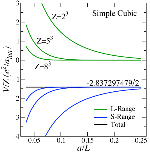
The Ewald construction is a powerful method that may be tested in a variety of ways. First, one may compare against well known results for the Coulomb energy of simple crystals. Second, whereas the Ewald construction introduces a dependence on the smearing parameter $a$, the “bare” Coulomb potential should be insensitive to it—as long as $a$ is neither too big nor too small. We have implemented such ideas in Fig. 7 where the Coulomb energy of a system consisting of $Z$ protons localized to the sites of a simple cubic lattice and immersed in a uniform electron background has been computed. The figure displays the competition between the long-range (repulsive) and the short-range (attractive) contributions to the Coulomb energy as a function of the smearing parameter $a$ and number of protons. The energy is given in units of $e^{2}/a_{\rm latt}$, where $a_{\rm latt}\!=\!\rho_{Z}^{1/3}$ is the lattice constant and $\rho_{Z}$ is the proton density. We obtain for all values of $a$ and all system sizes an energy per particle of $-2.837297479/2$, where $2.837297479$ is the Madelung constant for a simple-cubic crystal Brush et al. (1966). Remarkably, the Ewald method can already reproduce the exact answer (up to nine significant figures!) for a system with two protons per side.

Figure 7: (Color online) Coulomb energy per particle together with its long- and short-range contributions for a simple cubic lattice of $Z$ protons immersed in a neutralizing and uniform electron background. The Coulomb energy is given in units of $e^{2}/a_{\rm latt}$ ($a_{\rm latt}$ is the lattice constant) and the dimensionless Madelung constant for a simple cubic lattice is equal to $2.837297479$ Brush et al. (1966).

References

- Weber (1999) F. Weber, Pulsars as Astrophysical Laboratories for Nuclear and Particle Physics (Institute of Physics Publishing, Bristol, UK, 1999).
- Glendenning (2000) N. K. Glendenning, Compact Stars (Springer-Verlag New York, 2000).
- Piekarewicz (2009) J. Piekarewicz, AIP Conf. Proc. 1182, 937 (2009).
- Horowitz and Piekarewicz (2001) C. J. Horowitz and J. Piekarewicz, Phys. Rev. Lett. 86, 5647 (2001).
- Baym et al. (1971) G. Baym, C. Pethick, and P. Sutherland, Astrophys. J. 170, 299 (1971).
- Ruester et al. (2006) S. B. Ruester, M. Hempel, and J. Schaffner-Bielich, Phys. Rev. C73, 035804 (2006).
- Roca-Maza and Piekarewicz (2008) X. Roca-Maza and J. Piekarewicz, Phys. Rev. C78, 025807 (2008).
- Ravenhall et al. (1983) D. G. Ravenhall, C. J. Pethick, and J. R. Wilson, Phys. Rev. Lett. 50, 2066 (1983).
- Hashimoto et al. (1984) M. Hashimoto, H. Seki, and M. Yamada, Prog. Theor. Phys. 71, 320 (1984).
- Fetter and Walecka (1971) A. L. Fetter and J. D. Walecka, Quantum Theory of Many Particle Systems (McGraw-Hill, New York, 1971).
- Jamei et al. (2005) R. Jamei, S. Kivelson, and B. Spivak, Phys. Rev. Lett. 94, 056805 (2005).
- Oyamatsu and Iida (2007) K. Oyamatsu and K. Iida, Phys. Rev. C75, 015801 (2007).
- Horowitz et al. (2004a) C. J. Horowitz, M. A. Perez-Garcia, and J. Piekarewicz, Phys. Rev. C69, 045804 (2004a).
- Horowitz et al. (2004b) C. J. Horowitz, M. A. Perez-Garcia, J. Carriere, D. K. Berry, and J. Piekarewicz, Phys. Rev. C70, 065806 (2004b).
- Horowitz et al. (2005) C. J. Horowitz, M. A. Perez-Garcia, D. K. Berry, and J. Piekarewicz, Phys. Rev. C72, 035801 (2005).
- Watanabe et al. (2003) G. Watanabe, K. Sato, K. Yasuoka, and T. Ebisuzaki, Phys. Rev. C68, 035806 (2003).
- Watanabe et al. (2005) G. Watanabe, T. Maruyama, K. Sato, K. Yasuoka, and T. Ebisuzaki, Phys. Rev. Lett. 94, 031101 (2005).
- Watanabe et al. (2009) G. Watanabe, H. Sonoda, T. Maruyama, K. Sato, K. Yasuoka, et al., Phys. Rev. Lett. 103, 121101 (2009).
- Maruyama et al. (2005) T. Maruyama, T. Tatsumi, D. N. Voskresensky, T. Tanigawa, and S. Chiba, Phys. Rev. C72, 015802 (2005).
- Avancini et al. (2008) S. Avancini, D. Menezes, M. Alloy, J. Marinelli, M. Moraes, et al., Phys. Rev. C78, 015802 (2008).
- Avancini et al. (2009) S. Avancini, L. Brito, J. Marinelli, D. Menezes, M. de Moraes, et al., Phys.Rev. C79, 035804 (2009).
- Newton and Stone (2009) W. Newton and J. Stone, Phys. Rev. C79, 055801 (2009).
- Shen et al. (2011) G. Shen, C. Horowitz, and S. Teige, Phys. Rev. C83, 035802 (2011).
- Allen and Tildesley (1987) M. P. Allen and D. J. Tildesley, Computer Simulation of Liquids (Oxford University Press Inc., New York, 1987).
- Frenkel and Smit (1996) D. Frenkel and B. Smit, Understanding Molecular Simulations (Academic Press, San Diego, 1996).
- Vesely (2001) F. J. Vesely, Computational Physics: An Introduction (Kluwer Academic, New York, 2001).
- Ewald (1921) P. P. Ewald, Ann. Phys. 369, 253 (1921).
- Toukmaji and Board (1996) A. Y. Toukmaji and J. A. Board, Computer Physics Communications 95, 73 (1996).
- Pathria (1996) R. K. Pathria, Statistical Mechanics (Butterworth-Heinemann, Oxford, 1996), 2nd ed.
- Horowitz and Berry (2008) C. J. Horowitz and D. K. Berry, Phys. Rev. C78, 035806 (2008).
- Brush et al. (1966) S. G. Brush, H. L. Sahlin, and E. J. Teller, J. Chem. Phys. 45, 2102 (1966).