The Phase Transition for Dyadic Tilings

Abstract.

A dyadic tile of order $n$ is any rectangle obtained from the unit square by $n$ successive bisections by horizontal or vertical cuts. Let each dyadic tile of order $n$ be available with probability $p$, independently of the others. We prove that for $p$ sufficiently close to $1$, there exists a set of pairwise disjoint available tiles whose union is the unit square, with probability tending to $1$ as $n\to\infty$, as conjectured by Joel Spencer in 1999. In particular we prove that if $p=7/8$, such a tiling exists with probability at least $1-(3/4)^{n}$. The proof involves a surprisingly delicate counting argument for sets of unavailable tiles that prevent tiling.

1. Introduction

A dyadic tile of order $n$ is a rectangle of the form

$$\Bigl{[}\frac{a}{2^{i}},\frac{a+1}{2^{i}}\Bigr{]}\times\Bigl{[}\frac{b}{2^{j}},\frac{b+1}{2^{j}}\Bigr{]},$$

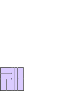
where $a,b,i,j$ are integers and $i+j=n$. We consider only tiles that are subsets of the unit square $[0,1]^{2}$, which is to say that $0\leq a<2^{i}$ and $0\leq b<2^{j}$. The tiles of order $n$ come in $n+1$ different shapes, each shape corresponding to a particular choice of $i$ and $j$. There are $2^{n}$ tiles of each shape, and thus in total $(n+1)\,2^{n}$ tiles of order $n$. A tiling of a rectangle $R$ is a set of tiles whose union is $R$ and whose interiors are pairwise disjoint. Figure 2 shows a tiling of the unit square by tiles of order 3; for visual clarity we illustrate tiles by rectangles with rounded corners, slightly smaller than their true sizes.

Figure 1. A dyadic tiling by order-3 tiles.

Figure 2. Tiling probabilities $T_{n}(p)$ for $n=0,1,2$.

Suppose that each tile of order $n$ is available with probability $p$ independently of the other tiles. Let $T_{n}(p)$ denote the probability that there exists a set of available order-$n$ tiles that constitutes a tiling of the unit square $[0,1]^{2}$. For example $T_{0}(p)=p$ trivially, and $T_{1}(p)=2p^{2}-p^{4}$ since each of the vertical and horizontal tilings is available with probability $p^{2}$ and both are available with probability $p^{4}$. A more involved calculation shows that $T_{2}(p)=7p^{4}-8p^{6}-4p^{7}+p^{8}+8p^{9}-4p^{11}+p^{12}$ (the term $7p^{4}$ corresponds to the $7$ distinct tilings by order-$2$ tiles). The functions $T_{0},T_{1},T_{2}$ are plotted in Figure 2.

It is natural to define the critical probability

$$p_{c}:=\inf\big{\{}p:\lim_{n\to\infty}T_{n}(p)=1\big{\}}.$$

Joel Spencer asked in 1999 whether $p_{c}<1$ (personal communication). The main result of this paper is an affirmative answer to this question. In particular we show the following.

Theorem 1.

We have

$$T_{n}(7/8) \geq 1-(3/4)^{n};$$

$$T_{n}(6/7) \geq 1-(16/17)^{n};$$

$$T_{n}(0.8560310279) \geq 1-(0.999998)^{n}.$$

In particular, $p_{c}\leq 0.8560310279$.

We explain in § 7 where these numbers come from. The first inequality can be checked by hand, while the second and third involve rigorous computer-assisted numerical methods. The bound $p_{c}\leq 0.856\cdots$ is the best that can be obtained with our method, but we believe that $p_{c}$ is smaller than this. Using standard sharp threshold technology, we also establish the following.

Theorem 2.

With $p_{c}$ defined as above,

$$\lim_{n\to\infty}T_{n}(p)=\begin{cases}0\quad\text{if $p<p_{c}$,}\\ 1\quad\text{if $p>p_{c}$}.\end{cases}$$

A straightforward argument proves the lower bound $p_{c}\geq(\surd 5{-}1)/2$ $=0.618\cdots$, and in fact this may be improved to

$$p_{c}\geq 0.785996.$$

It is likely that this bound could be improved still further—see § 2 for more information.

In $d$ dimensions we may similarly define an order-$n$ dyadic tile to be a product of $d$ dyadic intervals. Let each dyadic tile of volume $2^{-n}$ be available independently with probability $p$, and let $p_{c}(d)$ be the infimum of $p$ for which there is a tiling of the cube $[0,1]^{d}$ with probability tending to $1$ as $n\to\infty$. It is immediate that $p_{c}(d)$ is non-increasing in $d$ (since the product of any $d$-dimensional tiling with $[0,1]$ is a $(d+1)$-dimensional tiling), so Theorem 1 implies $p_{c}(d)<1$ for all $d\geq 2$. In dimension $3$ a simple argument gives the lower bound $p_{c}(3)\geq 1/8$ (see § 2), but for $d\geq 4$ we do not know whether $p_{c}(d)>0$.

A different model, of uniformly random dyadic tilings, was investigated by Janson, Randall and Spencer [4, 5]. Also see [6] for enumeration of tilings, and [1] for a related problem of random packing.

2. Preliminaries, and outline of proof

The following key observation is Theorem 1.1 of [5].

Lemma 3.

A dyadic tiling by tiles of order $n\geq 1$ consists either of tilings of the two horizontal rectangles $[0,1]\times[0,1/2]$ and $[0,1]\times[1/2,1]$, or tilings of the two vertical rectangles $[0,1/2]\times[0,1]$ and $[1/2,1]\times[0,1]$.

Proof.

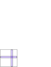
The only tiles that cross the median line $\{1/2\}\times[0,1]$ are those of the most horizontal shape, i.e. of the form $[0,1]\times[b/2^{n},(b+1)/2^{n}]$. Similarly the only tiles that cross $[0,1]\times\{1/2\}$ are of the most vertical shape. There cannot be tiles of both these shapes in a tiling, since they intersect (see Figure 3). ∎

We remark that the analogous statement to Lemma 3 fails in dimensions greater than $2$: see Figure 4 for a counterexample in dimension $3$.

Figure 3. A horizontal and a vertical tile intersect, and therefore cannot both be present in a tiling.

Figure 4. A dyadic tiling of the unit cube in which no half of the cube is tiled. Six tiles of dimensions $1\times\tfrac{1}{2}\times\tfrac{1}{4}$ (with various orientations) are shown, and the remaining space is filled by two $\tfrac{1}{2}\times\tfrac{1}{2}\times\tfrac{1}{2}$ cubes.

Corollary 4.

We have $T_{n+1}(p)\leq 2T_{n}(p)^{2}$.

Proof.

A tiling of a rectangle such as $[0,1]\times[0,1/2]$ by order $n+1$ tiles is isomorphic under an obvious affine transformation to a tiling of the unit square by order-$n$ tiles. Therefore the probability that the two horizontal rectangles $[0,1]\times[0,1/2]$ and $[0,1]\times[1/2,1]$ can both be tiled by available order-$(n+1)$ tiles is $T_{n}(p)^{2}$, and similarly for the two vertical rectangles $[0,1/2]\times[0,1]$ and $[1/2,1]\times[0,1]$. The inequality now follows from Lemma 3. ∎

Corollary 5.

For any given $p$, if there is an $n$ such that $T_{n}(p)<1/2$, then $\lim_{n\to\infty}T_{n}(p)=0$.

Proof.

This is immediate from Corollary 4.∎

We remark that the threshold $1/2$ in Corollary 5 can be improved (although this will not be needed). Consider the event $T^{\textrm{vert}}$ that there is a tiling by available order-$n$ tiles of both vertical halves of the unit square, and the event $T^{\textrm{horiz}}$ that there is a tiling of both horizontal halves. Since $T^{\textrm{vert}}$ and $T^{\textrm{horiz}}$ are increasing events, by the Harris-FKG inequality [3],

$$\mathbb{P}(T^{\textrm{horiz}}\cap T^{\textrm{vert}})\geq\mathbb{P}(T^{\textrm{horiz}})\,\mathbb{P}(T^{\textrm{vert}})=T_{n}(p)^{4}.$$

Thus we get the inequality $T_{n+1}(p)\leq 2T_{n}(p)^{2}-T_{n}(p)^{4}$. It follows that if $T_{n}(p)<(\surd 5-1)/2$ then $\lim_{n\to\infty}T_{n}(p)=0$.

Since $T_{0}(p)=p$, Corollary 5 immediately implies $p_{c}\geq 1/2$, and the enhancement described above gives $p_{c}\geq(\surd 5-1)/2$.

Corollary 5 also implies that $T_{n}(p_{c})\geq 1/2$ for all $n$ (and in fact, $1/2$ may be replaced with $(\surd 5-1)/2$). Indeed, if $T_{n}(p_{c})<1/2$ then, by the continuity of $T_{n}$ (which is a polynomial), for some $p>p_{c}$ we would also have $T_{n}(p)<1/2$. Corollary 5 then shows that $T_{n}(p)\to 0$, in contradiction to $p>p_{c}$.

Covering and lower bounds

Next we briefly discuss covering. This basic concept will not be needed for our proof of Theorem 1, but it motivates parts of the proof and also yields improved lower bounds on $p_{c}$. If some point $x\in[0,1]^{2}$ is not covered by any available tile, then clearly there is no tiling by available tiles. Each of the the $4^{n}$ squares of size $2^{-n}\times 2^{-n}$ is uncovered with probability $(1-p)^{n+1}$, and it follows that for $p>3/4$ there are no uncovered points with high probability as $n\to\infty$. A standard second-moment argument shows furthermore that for $p<3/4$ there are uncovered points with high probability, implying $p_{c}\geq 3/4$.

The absence of uncovered points is necessary but not sufficient for tiling; see Figure 5 for an example. Therefore the above argument cannot yield an upper bound on $p_{c}$. In fact, it may be shown that $p_{c}$ (the critical point for tiling) is strictly greater than $3/4$ (the critical point for covering), as follows. Let $n\geq 1$. A friend of an order-$n$ tile $s$ is an order-$n$ tile $t$ such that $s\cup t$ is an order-$(n-1)$ tile. Observe that in any dyadic tiling, every tile has some friend also present in the tiling. Call a $2^{-n}\times 2^{-n}$ square bad if every available tile that covers it has no available friend. Thus a bad square prevents tiling. Each square is bad with probability $[1-p+p(1-p)]^{2}[1-p+p(1-p)^{2}]^{n-1}$, and a second-moment argument again goes through to show that if $1-p+p(1-p)^{2}>1/4$ then bad squares exist with high probability as $n\to\infty$. This gives $p_{c}\geq 0.785996$. It seems likely that the bound could be further improved by considering more complicated local obstacles to tiling.

Figure 5. A configuration that covers but does not tile.

Before moving on to discuss the proof of Theorem 1 we explain the claimed lower bound on $p_{c}(3)$ in dimension $3$. We cannot use covering: for $d\geq 3$, every point of $[0,1]^{d}$ is covered with high probability for every $p>0$ (by a first-moment argument). However, in a tiling of the cube $[0,1]^{3}$ by order-$n$ tiles, intersecting each tile with a fixed face of the cube yields a tiling of the face by $2$-dimensional tiles of orders $n$ or lower, and furthermore any such $2$-dimensional tile can arise from exactly one possible $3$-dimensional order-$n$ tile. Let $L_{n}(p)$ be the probability that the square $[0,1]^{2}$ is tiled by available tiles when each tile of order $n$ or lower is available independently with probability $p$. Thus the $3$-dimensional tiling probability $T_{n}^{(3)}(p)$ is at most $L_{n}(p)$. Similarly to Corollary 4, we obtain

$$L_{n+1}(p)\leq p+2L_{n}(p)^{2},$$

and it follows that if $p<1/8$ then $\limsup_{n\to\infty}L_{n}(p)<1$. Thus $p_{c}(3)\geq 1/8$. (Again, this bound could likely be improved).

Outline of proof

We next describe the main ideas behind the proof of Theorem 1. The basic strategy is simple and standard: we show that if $[0,1]^{2}$ is not tiled, then a certain combinatorial structure of unavailable tiles must exist; by counting such structures (weighted according to the number of unavailable tiles) we then show that for $p$ sufficiently close to $1$ their expected number is small. The challenge, of course, is to find a suitable class of combinatorial structures.

As discussed above, uncovered points (or similar structures) are not suitable for our purpose, because their absence does not imply existence of a tiling. Instead we proceed as follows. If the unit square is not tileable by available tiles, then by Lemma 3, one of the two horizontal halves and one of the two vertical halves must also be not tileable; see e.g. Figure 6(a). We can then iterate: each of the two non-tileable halves must itself have two non-tileable halves, and so on until we reach some “blocking set” of unavailable tiles of order $n$, whose unavailability is sufficient to prevent a tiling of the square. For example, Figure 6(b) shows one possibility at order $2$.

If at every stage of the above procedure all the resulting non-tileable tiles were distinct, then the proof would be straightforward: the number of unavailable tiles in the final blocking set would be $2^{n}$, and the number of possible blocking sets would be at most $4^{2^{n}-1}$ (there are $4$ choices for the pairs of halves of each tile), and $4^{2^{n}-1}(1-p)^{2^{n}}$ is small for $p$ sufficiently close to $1$.

However, the tiles resulting from the above iterative procedure are not necessarily distinct. Even at order $2$, there is a blocking set of $3$ (as opposed to $4$) tiles; see Figure 6(c). A blocking set with fewer tiles signals a potential difficulty, since the probability that they are all unavailable is larger. However, the number of possible outcomes with fewer tiles may also be smaller. In particular, the minimum number of unavailable tiles of order $n$ needed to prevent tiling the unit square is $n+1$, and in fact the sets of $n+1$ tiles that achieve this are precisely those whose mutual intersection is some $2^{-n}\times 2^{-n}$ square. Therefore the number of such minimum-size blocking sets is only $4^{n}$, and ruling them out for large $p$ simply amounts to the earlier “covering” calculation.

Figure 6. (a) Two order-$1$ tiles that together block the unit square. (b) Four order-$2$ tiles that block the tiles in (a). (c) Three order-$2$ tiles that block the tiles in (a).

The issue now is that there are many intermediate blocking sets with numbers of tiles between $n+1$ and $2^{n}$. We must analyze these possibilities taking into account both the number of choices and the resulting numbers of tiles (and these two quantities must be weighed against each other). To achieve this, we will organize blocking sets into chains. A chain is the set of all tiles of a given order that contain some fixed tile of some higher order. (Equivalently, it is one of the minimum blocking sets discussed above, but within some tile of intermediate order rather than the whole square). For example, the set in Figure 6(c) is a chain of 3 tiles, while that in (b) can be expressed as a union of 2 chains each consisting of 2 tiles. Although our eventual interest lies in the cardinality of the blocking set resulting from the iterative procedure, we will count the possible outcomes using a generating function of two parameters, corresponding to numbers of tiles and numbers of chains. The resulting counting argument is short but somewhat mysterious. The inclusion of both parameters appears to be not merely a technical requirement but a fundamental one: we do not know how to proceed by counting tiles alone.

Another complication is as follows. In the iterative procedure for finding blocking sets outlined above, several choices may be possible. It is possible for example that both horizontal halves of a tile are non-tileable, and we must choose one of them. It turns out that how we do this is crucial. We will impose the rule that we always make the choice that minimizes the resulting number of chains. For example, starting from the situation of Figure 6(a), we choose the blocking set in (c) in preference to the one in (b). (We might however be forced to take the one in (b) if the bottom-right $\tfrac{1}{2}\times\tfrac{1}{2}$ square is tileable). With this rule, it will turn out that the collection of chains produced by the iterative procedure is pairwise disjoint. Without it, chains could intersect (or indeed coincide); this would result in a reduction in the number of tiles in the blocking set, again adversely affecting the resulting bound on the probability that they are all unavailable. Combined with the counting argument mentioned earlier, this disjointness of chains suffices to give a bound of the required form.

Organization

The article is organized as follows. In § 3 below we prove the sharp threshold result, Theorem 2. The remainder of the article is devoted to the proof of Theorem 1. In § 4 we introduce chains of tiles, and prove some properties. In § 5 we arrange chains into chain trees. These are the “blocking configurations” at the heart of the proof: if the unit square is not tiled, then there is a blocked chain tree, and we can bound the probability of this event by counting chain trees. In § 6 we prove that non-tileability implies the existence of a chain tree of a special type which is guaranteed to have all its chains disjoint, as discussed above. Finally, in § 7 we employ generating functions to perform the necessary counting argument. We conclude with some open problems.

3. Sharp threshold

We will deduce Theorem 2 from Corollary 5 together with the following result of Friedgut and Kalai. In their paper [2] this is Theorem 2.1, modified according to the comment after Corollary 3.5. Here $A$ is a subset of the hypercube $\{0,1\}^{N}$, endowed with the product probability measures $\mathbb{P}_{p}$.

Theorem (Friedgut and Kalai; [2]).

Let $A$ be increasing and invariant under the action on $\{1,\ldots,N\}$ of a group with orbits of size at least $m$. If $\mathbb{P}_{p}(A)>\epsilon$ then $\mathbb{P}_{q}(A)>1-\epsilon$ for $q=p+c\log(1/2\epsilon)/\log m$ and an absolute constant $c$.

(For our application, all that matters is that the difference $q-p$ appearing in the above theorem tends to $0$ as $m\to\infty$. As noted in [2], this can also be deduced from earlier results of Russo [7] or Talagrand [8].)

Proof of Theorem 2.

The second claim of Theorem 2 is immediate since $T_{n}(p)$ is increasing in $p$, so we turn to the first claim. Let $S$ be the set of order-$n$ tiles, and let $A\subset\{0,1\}^{S}$ be the event that the unit square is tileable by available tiles, where $0$ and $1$ represent unavailable and available respectively. Thus $T_{n}(p)=\mathbb{P}_{p}(A)$. We will show below that $A$ is invariant under the action of a group of permutations of tiles with orbits of size $2^{n}$.

Suppose that $p<p_{c}$, and let $p<q<p_{c}$. The definition of $p_{c}$ implies that $T_{n}(q)<1-\epsilon$ for some $0<\epsilon<1/2$ and infinitely many $n$. Since $c\log(1/2\epsilon)/\log(2^{n})\to 0$ as $n\to\infty$, the Friedgut-Kalai theorem then implies that $T_{n}(p)\leq\epsilon<1/2$ for some $n$. Corollary 5 then gives $\lim_{n\to\infty}T_{n}(p)=0$ as required.

It remains to exhibit a group of symmetries of $A$ with orbits of size $2^{n}$. Consider the mapping $f_{k}:[0,1]\to[0,1]$ that changes the $k^{\textrm{th}}$ digit in the binary expansion, leaving the rest unchanged. It is easy to see that for any $k$, the maps $(x,y)\mapsto(f_{k}(x),y)$ and $(x,y)\mapsto(x,f_{k}(y))$ both permute dyadic tiles, since specifying a dyadic tile is equivalent to specifying several initial digits in each of $x$ and $y$ (see Figure 7).

Figure 7. The symmetry $(x,y)\mapsto(f_{1}(x),y)$ swaps the left and right halves of the square, and acts on the $12$ tiles of order $2$.

Since these maps preserve intersection of tiles, they also preserve tilings, and hence they preserve $A$. By applying a sequence of such maps we can change any tile of a given shape to any other tile of the same shape, and so the generated group has orbits of size $2^{n}$. ∎

In dimensions $d\geq 3$ we do not know whether the analogue of Theorem 2 holds, since our proof relies on Lemma 3. However, we can still apply the Friedgut-Kalai theorem as above for all $d$. Hence the argument for the bound $p_{c}(3)\geq 1/8$ also gives that $T_{n}^{(3)}(p)\to 0$ for $p<1/8$.

4. Blocked tiles and chains

Our next objective is to prove Theorem 1. We start with some important definitions.

Given a classification of the order-$n$ tiles into available and unavailable, we say that a tile of order $k\leq n$ is tileable if it can be tiled by available tiles of order $n$. Otherwise it is blocked (in particular, tiles of order $n$ are blocked if and only if they are unavailable). The two order-$(k+1)$ tiles that are obtained by bisecting an order-$k$ tile with a horizontal cut are its horizontal children, and similarly the two tiles that are obtained by cutting vertically are its vertical children.

Lemma 6.

A tile of order less than $n$ is blocked if and only if at least one of its horizontal children and at least one of its vertical children is blocked.

Proof.

This is the contrapositive of Lemma 3 (applied to a tile rather than the whole square). ∎

Our goal is to arrange sets of blocked order-$k$ tiles into chains. If $s$ and $t$ are tiles of order $k$ whose interiors intersect, then the chain $[s,t]$ is the set of all order-$k$ tiles that contain their intersection $s\cap t$.

A chain contains a most horizontal and a most vertical tile (these are $s$ and $t$), and exactly one tile of each intermediate shape. Two order-$k$ tiles are called adjacent if their intersection is an order-$(k+1)$ tile. A bond of a chain is a pair of adjacent tiles in the chain. Thus the number of bonds of a chain is one less than the number of tiles. Observe also that a chain is precisely a directed path in the graph whose vertices are all order-$k$ tiles, with adjacent pairs connected by an edge directed towards the more vertical tile. (In fact, this graph may be viewed as a lamplighter graph corresponding to binary lamps on a path of length $n$; see e.g. [9] for a definition.)

Figure 8. A chain consisting of the three order-$3$ tiles that contain an order-$5$ tile.

We now define the notion of successors of chains. Let $[s,t]$ be an order-$k$ chain, with $s$ the horizontal end-tile and $t$ the vertical end-tile. A successor of the chain $[s,t]$ is any set of tiles of order $k+1$ with the property that it includes exactly one horizontal child and exactly one vertical child of every element of $[s,t]$.

The idea of the last definition is that a successor of $[s,t]$ is a minimal set with the property that if it were blocked, then $[s,t]$ would be blocked, according to Lemma 6. (We call a set of tiles blocked if all its tiles are blocked). If a chain of order less than $n$ is blocked, then it possesses some blocked successor. The last fact is not immediately obvious, because of the requirement that a successor include exactly one child of each type. However, it follows from Figure 9 and the proof of Lemma 7 below. We will eventually need a somewhat stronger statement—see Lemma 9 in § 6.

Figure 9. Tiles involved in possible successors of a chain. White discs are the $4$ tiles of a chain of order $k$ (with $3$ bonds). Black discs are tiles of order $k+1$. Adjacent tiles are connected by dashed arrows towards the more vertical tile. Solid arrows connect a tile to its children (with horizontal children to the left, and vertical children to the right).

A key ingredient in our proof is to classify the possible successors of a given chain. We say that two chains are separate if they are disjoint, and no tile of one is adjacent to any tile of the other. (This implies in particular that their tiles cannot be partitioned into one or two chains in any other way). Here and elsewhere, disjointness of chains of means simply that they have no tiles in common; the tiles themselves are permitted to intersect one another.

Lemma 7.

Any successor of a chain can itself be uniquely expressed as a union of pairwise separate chains. For a chain of $b$ bonds, any successor has exactly $b+1$ bonds in total, and there are $4\binom{b}{r}$ possible successors that consist of $r+1$ separate chains, for each $r=0,\dots,b$.

Proof.

The key observations are illustrated in Figure 9. Each tile in a chain $[s,t]$ has two horizontal children and two vertical children, but not all these children are distinct. Specifically, if $u,v$ are two adjacent tiles of the chain $[s,t]$ (with $u$ the more horizontal), then there is a unique tile that is both a vertical child of $u$ and a horizontal child of $v$, namely the intersection $u\cap v$. Aside from such intersections (one for each bond of $[s,t]$), all children of the tiles of $[s,t]$ are distinct. Note also that any horizontal child of a given tile is adjacent to any vertical child, and these are the only adjacencies among children of the tiles of $[s,t]$.

We can now consider possible successors. Firstly, if for each bond in $[s,t]$ we take the intersection tile, and in addition we choose one horizonal child $s^{\prime}$ of $s$ and one vertical child $t^{\prime}$ of $t$, then we obtain one possible successor of $[s,t]$—in fact, this successor is precisely the order-$(k+1)$ chain $[s^{\prime},t^{\prime}]$. We call a successor consisting of a single chain simple. See Figure 10(b) for an example. There are $2^{2}=4$ possible simple successors of a given chain, since there are two possibilities each for $s^{\prime}$ and $t^{\prime}$.

On the other hand, consider a successor that does not include $u\cap v$. (In the forthcoming application to blocked chains, it will be necessary to consider such a case if $u\cap v$ is tileable). In that case the successor must include the other vertical child of $u$, namely $\overline{u\setminus v}$ (where the bar denotes topological closure), and similarly it must include $\overline{v\setminus u}$. Now if, for instance, for each of the other bonds of $[s,t]$ we select the intersection tile as before (and we select the same end tiles $s^{\prime},t^{\prime}$), the resulting successor can be expressed as the union of the two separate chains $[s^{\prime},\overline{u\setminus v}]$ and $[\overline{v\setminus u},t^{\prime}]$. We say that a split occurred at the bond $(u,v)$. In general, each bond of $[s,t]$ may or may not be split, and the resulting successor can always be uniquely expressed as a union of separate chains, with $r$ splits resulting in $r+1$ chains. Combined with the $4$ choices of the end tiles $s^{\prime}$ and $t^{\prime}$, this gives the claimed enumeration. ∎

Figure 10. (a) A chain of tiles of order $2$. (b) A simple successor of the chain. (c) A split successor of the chain, with the same end tiles.

See Figure 10 for an example—if one splits the order-2 chain $[s,t]=\{s,u,t\}$ in (a) between tiles $u$ and $t$ (i.e. between the square and the vertical tile), one gets two chains shown in (c), the first being a simple successor of $[s,u]$ and the second a simple successor of $[t,t]$.

The above ideas will be applied as follows. If every tile of a chain of order less than $n$ is blocked, then the chain must have a successor each of whose tiles is blocked, by Lemma 6. Thus, if the unit square is blocked, then we can start from the chain consisting only of the unit square, and repeatedly find successors until we reach a set of chains of order $n$ consisting entirely of unavailable tiles. The set of tiles in these chains has the property that if they are unavailable then the square is not tileable. Next we want to count the possible outcomes of such a process.

5. Chain trees

We next introduce an object called a chain tree, which formalizes the idea of an iterative construction of a blocking set of tiles. Note however that the definition itself will be purely combinatorial, and will not refer to availability of tiles.

A chain tree of depth $n$ is a rooted tree of depth $n$ in which each vertex is labeled with a chain of tiles (where we allow the possibility that distinct vertices are labeled with the same chain or intersecting chains), and with the following properties.

1. The root corresponds to the order-$0$ chain consisting only of the unit square.

2. For any vertex $v$ at level less than $n$, the children of $v$ correspond to pairwise separate chains whose union is a successor of the chain at $v$.

Note that each vertex at level $k$ corresponds to a chain of order $k$, and the leaves of the tree correspond to chains of order $n$. Observe also that stripping the leaves from a chain tree of depth $n+1$ results in a chain tree of depth $n$.

For a chain tree $T$ of depth $n$, let $c(T)$ be the number of leaves, and $t(T)$ the total number of tiles in chains at the leaves (counted with multiplicity; in other words the sum of the cardinalities of the chains rather than the number of distinct tiles that occur). It is also convenient to let $b(T)=t(T)-c(T)$ be the total number of bonds in the chains at the leaves (also counted with multiplicity). For example, for the simplest chain trees consisting only of simple successors, and exactly one chain at each level, we have $c(T)=1$ and $b(T)=n$.

We will need to enumerate chain trees of depth $n$ weighted according to the number of leaf tiles. To this end we define the two-variable polynomial

$$f_{n}=f_{n}(q,z):=\sum_{T}q^{b(T)}z^{c(T)},$$

where the sum is over all chain trees of depth $n$. For instance, $f_{0}=z$, since the unique depth zero chain tree consists of a single chain containing a single tile (so no bonds). At order $1$ there are $4$ possible successors to this chain, and there cannot yet be any splitting. Hence $f_{1}=4qz$. At the next level, any given order-$1$ chain has $4$ possible simple successors, and $4$ possible split successors into $2$ chains (each having one bond). Hence $f_{2}=4(4q^{2}z+4q^{2}z^{2})=16q^{2}z(1+z)$.

Next we will see how $f_{n}$ is related to the tiling probability $T_{n}$.

6. The principal chain tree

In this section we will prove the following.

Proposition 8.

For all $n,p$ we have

(1) $$1-T_{n}(p)\leq f_{n}(1-p,1-p).$$

Then in § 7 we will analyze the asymptotic behaviour of $f_{n}(q,q)$ for $q$ small, which will enable us to deduce Theorem 1.

To motivate the proof of Proposition 8, observe that

$$f_{n}(q,q)=\sum_{T}q^{t(T)},$$

which enumerates chain trees weighted by $q$ to the number of tiles at depth $n$. If we set $q=1-p$, and if it happens that the chains at depth $n$ of $T$ are pairwise disjoint, then the term $q^{t(T)}$ is the probability that all their constituent tiles are unavailable.

If it were the case that the leaves of a chain tree always corresponded to pairwise disjoint chains, then Proposition 8 would follow immediately from Lemma 6 by the argument outlined at the end of § 4. However, there do exist chain trees with repeated tiles (see Figure 11 for an example).

Figure 11. Part of a chain tree with a duplicate tile (arrows are from a node to its children in the tree). The $\frac{1}{4}\times\frac{1}{4}$ bottom left corner tile is contained in both the top and bottom leaves.

Therefore, we will define a special class of chain trees whose chains will turn out to be disjoint. They will be constructed by iteratively finding blocked successors to each blocked chain, as discussed earlier, but with the additional restriction that we split only where necessary. More formally, given a designation of all order-$n$ tiles as available and unavailable, we call a depth-$n$ chain tree $T$ a principal chain tree if in addition to conditions (I) and (II), it satisfies the following.

1. Each tile in each chain of $T$ is blocked.

2. If the chain corresponding to some vertex contains a bond $(u,v)$ for which the tile $u\cap v$ is blocked, then one of its children contains $u\cap v$ in its chain (i.e. there is no split at this bond).

Lemma 9.

If $[0,1]^{2}$ is blocked, then there exists a principal chain tree.

Proof.

Start with the blocked chain containing only $[0,1]^{2}$, and iteratively find a blocked successor of each previously-constructed chain, splitting at a bond $(u,v)$ only when the tile $u\cap v$ is tileable. ∎

The key fact about principal chain trees is the following.

Lemma 10.

In a principal chain tree, the chains corresponding to distinct vertices are disjoint.

Proof.

The proof relies on two observations. First, consider the graph whose vertices are all tiles (of all orders) that contain as a subset some fixed tile $w$, and with a directed edge from a tile to its children in this set. This graph is isomorphic to a rectangular portion of the oriented square lattice $\mathbb{Z}^{2}$, as shown in Figure 12. If $w$ has shape $2^{-a}\times 2^{-b}$, the point $(i,j)$ corresponds to the unique tile of shape $2^{-i}\times 2^{-j}$ that contains $w$, for each $0\leq i\leq a$ and $0\leq j\leq b$. (In the figure, the first coordinate increases from top to bottom, and the second from left to right). Adjacent pairs of tiles correspond to points differing by the diagonal vector $(-1,1)$. Thus, a chain all of whose tiles contain $w$ corresponds to an interval on some diagonal in the lattice.

Figure 12. The tiles that contain $w$. Solid arrows point from tiles to their children, and dashed arrows connect adjacent pairs of tiles, pointing towards the more vertical tile. A chain is highlighted.

Second, we observe that paths in a chain tree may be mapped to paths in the lattice in the following way. Recall that different vertices in the chain tree may a priori be labeled with the same chain (although the present proof will in particular rule this out), so we must be careful to distinguish between vertices in the tree and their associated chains. Suppose that a tile $w$ is contained in a chain corresponding to some vertex $x$ in a chain tree. Consider the unique self-avoiding path $\pi$ from $x$ to the root in the chain tree. The chain of the parent vertex of $x$ in this path must contain either the horizontal parent or the vertical parent of $w$ (possibly both). (The horizontal parent of $w$ is the unique tile that has $w$ as a vertical child, and the vertical parent is defined similarly). Iterating this, we find a sequence of blocked tiles, each a parent of the previous one, starting at $w$ and ending at $[0,1]^{2}$. We call such a sequence an ancestry of $w$. Each tile of an ancestry belongs to the chain of the corresponding vertex of the path $\pi$. Each tile in an ancestry contains $w$, and an ancestry corresponds to a (backwards) directed path in the lattice.

Now suppose for a contradiction that an order-$n$ tile $w$ occurs in two (not necessarily different) chains corresponding to different vertices at level $n$ of a principal chain tree. These vertices have a last common ancestor vertex in the chain tree, with a corresponding chain $C$. We can also find two ancestries of $w$ corresponding to its membership in the two initial chains, and each of them must include a tile in $C$; call these two tiles $s$ and $t$, and let $s_{+},t_{+}$ be their respective children in the two ancestries. By the choice of $C$, the tiles $s_{+}$ and $t_{+}$ must lie in the chains of two different children of $C$. Hence the chain tree must include a split at some bond of $C$ somewhere between $s$ and $t$. By property (IV) of a principal chain tree, this split must occur because some tile $u$ that is the intersection of two adjacent tiles in the chain $[s,t]\subseteq C$ is tileable. Note that $s$ and $t$ both contain $w$, hence so does every tile in $[s,t]$, and hence so does $u$.

Figure 13. The path of tileable tiles from $u$ must intersect one of the paths of blocked tiles from $s$ and $t$ to $w$, a contradiction.

The two ancestries of blocked tiles from $w$ to each of $s$ and $t$ correspond to directed paths in the square lattice, as indicated in Figure 13. (The two ancestries might a priori intersect, although aside from $s$ and $t$ their tiles occur in chains at distinct vertices in the chain tree). Now consider the tile $u$, which abuts some bond of the chain $[s,t]$ in the lattice as shown. By Lemma 6, either both horizontal or both vertical children of $u$ are tileable. (This is the only place where we use the “only if” direction of Lemma 6). Suppose that $u$ is strictly larger than $w$ in both width and height. Then $w$ is contained in one of $u$’s horizontal children and one of its vertical children, hence $u$ has a child that contains $w$ and is tileable. Iterating this argument until we reach a tile of the same width or height as $w$, we obtain a directed path of tileable tiles in the lattice, starting at $u$ and ending in the row or column containing $w$, as shown in Figure 13. Such a path must intersect one of the two blocked ancestry paths, giving a contradiction. ∎

Proof of Proposition 8.

Using Lemmas 9 and 10,

$$1-T_{n}(p) =\mathbb{P}\bigl{(}[0,1]^{2}\text{ is blocked}\bigr{)}$$

$$=\mathbb{P}(\text{there exists a principal chain tree})$$

$$\leq\sum_{T}(1-p)^{t(T)}\mathbf{1}[\text{$T$ has pairwise disjoint chains}]$$

$$\leq\sum_{T}(1-p)^{t(T)}$$

$$=f_{n}(1-p,1-p),$$

where the sums are over all chain trees of depth $n$. ∎

7. Analysis of the generating function

To complete the proof of Theorem 1, all that remains is to analyze the asymptotic behavior of $f_{n}$. Recall that this is the generating function for all possible chain trees of depth $n$—we will no longer be concerned with availability or principal chain trees.

Proposition 11.

The polynomials $f_{n}$ satisfy the recursion

(2) $$f_{n+1}(q,z)=f_{n}\bigl{(}q(1+z),4qz\bigr{)}.$$

Proof.

Given a chain tree $T$ of depth $n$, we may obtain a chain tree of depth $n+1$ by choosing a successor of each leaf chain of $T$ and adding the appropriate children. All chain trees of depth $n+1$ can be obtained (each exactly once) in this way.

Fix some chain of $\beta$ bonds, and for any successor $S$, write $b(S)$ for the number of bonds and $c(S)$ for the number of pairwise separate chains. Then by Lemma 7, the generating function of the possible successors is given by

(3) $$\sum_{S}q^{b(S)}z^{c(S)}=\sum_{r=0}^{\beta}\binom{\beta}{r}4q^{\beta+1}z^{r+1}=\big{[}q(1+z)\big{]}^{\beta}4qz,$$

where the sum is over all possible successors of the given chain.

Consider a depth-$n$ chain tree $T$ whose leaves have $c$ chains, $t$ tiles and $b=t-c$ bonds (counted with multiplicities, as before). This chain tree contributes a term $q^{b}z^{c}$ to $f_{n}(q,z)$. The possible extensions of $T$ to depth $n+1$ contribute various terms to $f_{n+1}(q,z)$, and since we may choose any successor for each leaf independently of the others, the sum of these terms is the product of expressions of the form (3) over the leaves of $T$. That is:

(4) $$\prod_{L}\bigl{[}q(1+z)\bigr{]}^{\beta(L)}4qz=\bigl{[}q(1+z)\bigr{]}^{b}(4qz)^{c},$$

where the product is over the leaves of $T$, and $\beta(L)$ is the number of bonds of the chain at leaf $L$.

The polynomial $f_{n+1}(q,z)$ is obtained by summing the expression in (4) over all chain trees of depth $n$. Therefore, it is obtained from $f_{n}(q,z)$ by replacing each term $q^{b}z^{c}$ with the term $[q(1+z)]^{b}(4qz)^{c}$. This gives (2). ∎

Corollary 12.

Fix $q$ and $z$ and write $f_{n}=f_{n}(q,z)$. For every $n$,

(5) $$\frac{f_{n+2}}{f_{n+1}}=\frac{f_{n+1}}{f_{n}}+f_{n+1}.$$

Proof.

For $n=0$, (5) is easily verified (recall that $f_{0}=z$, $f_{1}=4qz$, and $f_{2}=16q^{2}z(1+z)$). Now the two-variable rational function $R_{n}:=f_{n+2}/f_{n+1}-f_{n+1}/f_{n}-f_{n+1}$ satisfies the same recursion (2) as $f$, that is, $R_{n+1}(q,z)=R_{n}(q(1+z),4qz)$; this is immediate simply by substituting from (2) for each of $f_{n+3},f_{n+2},f_{n+1}$. It follows that $R_{n}$ is identically zero for every $n$. ∎

Next, we show how to control the asymptotic behaviour of solutions to the recursion (5).

Lemma 13.

Suppose that $a_{0},a_{1}>0$, and that the sequence $(a_{n})$ satisfies the recursion (5), in other words for every $n$,

(6) $$\frac{a_{n+2}}{a_{n+1}}=\frac{a_{n+1}}{a_{n}}+a_{n+1}.$$

If $X$ satisfies

(7) $$\frac{a_{k}}{a_{k-1}}+\frac{a_{k}}{1-X}\leq X<1,$$

for some $k$, then for every $n$ we have $a_{n+1}/a_{n}<X$ and so $a_{n}<a_{0}X^{n}$.

Proof.

Write $Q_{n}=a_{n}/a_{n-1}$. Observe that $a_{n}>0$ for all $n$, by induction. Therefore $Q_{n}$ is increasing in $n$. We need to prove that $Q_{n}<X$ for all $n\geq 1$. By (7) we have

$$Q_{k}<Q_{k}+\frac{a_{k}}{1-X}\leq X,$$

so the required inequality holds for $n=k$, and hence also for all $n<k$ since $Q_{n}$ is increasing. For $n>k$ we use induction. Suppose that $Q_{n}<X$ for all $n\leq m$, where $m\geq k$. By repeated application of (6),

$$Q_{m+1}=Q_{k}+\sum_{i=k}^{m}a_{i}.$$

On the other hand the inductive hypothesis gives $a_{i}\leq a_{k}X^{i-k}$ for $k\leq i\leq m$, so substituting into the last equation and using (7) gives

$$Q_{m+1}<Q_{k}+\frac{a_{k}}{1-X}\leq X.\qed$$

Corollary 14.

Let $0<q<1$, and define a sequence $(a_{n})_{n\geq 0}$ by $a_{0}=q$, $a_{1}=4q^{2}$, and

$$\frac{a_{n+2}}{a_{n+1}}=\frac{a_{n+1}}{a_{n}}+a_{n+1},\qquad n\geq 0$$

If for some $k$ we have $a_{k}<a_{k-1}$ and

(8) $$\Bigl{(}1-\frac{a_{k}}{a_{k-1}}\Bigr{)}^{2}\geq 4a_{k},$$

then for every $n$,

(9) $$f_{n}(q,q)\leq\Bigl{(}\frac{1+a_{k}/a_{k-1}}{2}\Bigr{)}^{n}.$$

Proof.

It is easy to verify that an $X$ satisfying the quadratic inequality (7) exists exactly when (8) holds, in which case $X=(1+a_{k}/a_{k-1})/2$ is a solution. Since $a_{0}=q<1$, Lemma 13 implies the result. ∎

Proof of Theorem 1.

We combine Corollary 14 with Proposition 8 for suitable values of $k$ and $q:=1-p$. With $q=1/8$ we get $a_{0}=1/8$ and $a_{1}=1/16$. Therefore (8) holds with equality for $k=1$, and (9) gives the first claim of Theorem 1.

Using arithmetic with rational numbers to avoid numerical errors, we have verified that for $q=1/7$, (8) is satisfied for $k=16$, and $(1+a_{16}/a_{15})/2$ is slightly smaller than $16/17$. This establishes the second claim of Theorem 1, but the calculation involves integers with more than $50000$ digits. Similarly, using interval arithmetic to avoid errors gives the third claim. ∎

For the above values of $q$, the bounds on $T_{n}(p)$ are not the best that can be obtained from our analysis. Using larger $k$ and the optimal bound from Lemma 13 yields slightly better exponential decay. For example, this gives $T_{n}(7/8)\geq 1-0.655^{n}$. We believe that the correct exponential decay is even faster, and that $p_{c}$ is strictly smaller than our bound.

Open problems

1. Does the tiling probability $T_{n}(p_{c})$ at the critical point have a limit as $n\to\infty$? If so, what is it? Is it $1$? (As remarked in § 2, such a limit must be at least $(\surd 5-1)/2$.)

2. Is there a phase transition in dimensions $d\geq 4$? I.e., is $p_{c}(d)$ strictly positive?

3. Is there a unique critical point in dimension $3$? I.e., does the tiling probability $T_{n}^{(3)}(p)$ tend to $0$ or $1$ as $n\to\infty$ according as $p<p_{c}(3)$ or $p>p_{c}(3)$. (As discussed in § 2 and 3, we know that there is a sharp transition for each $n$ in the sense that $T_{n}^{(3)}(p)$ increases from $\epsilon$ to $1-\epsilon$ over an interval of length $o(1)$ as $n\to\infty$, and that the location of this interval is bounded strictly away from $0$ and $1$. The question is whether the location converges or oscillates).

References

- [1] E. G. Coffman, Jr., G. S. Lueker, J. Spencer, and P. M. Winkler. Packing random rectangles. Probab. Theory Related Fields, 120(4):585–599, 2001. springer.com, columbia.edu/~egc.
- [2] E. Friedgut and G. Kalai. Every monotone graph property has a sharp threshold. Proc. Amer. Math. Soc., 124(10):2993–3002, 1996. ams.org.
- [3] T. E. Harris. A lower bound for the critical probability in a certain percolation process. Proc. Cambridge Philos. Soc., 56:13–20, 1960. cambridge.org.
- [4] S. Janson. Remarks to random dyadic tilings of the unit square, 2001. Preprint, math.uu.se/~svante.
- [5] S. Janson, D. Randall, and J. Spencer. Random dyadic tilings of the unit square. Random Structures Algorithms, 21(3-4):225–251, 2002. Random structures and algorithms (Poznan, 2001). wiley.com, math.uu.se/~svante.
- [6] J. C. Lagarias, J. H. Spencer, and J. P. Vinson. Counting dyadic equipartitions of the unit square. Discrete Math., 257(2-3):481–499, 2002. sciencedirect.com.
- [7] L. Russo. An approximate zero-one law. Z. Wahrsch. Verw. Gebiete, 61(1):129–139, 1982.
- [8] M. Talagrand. On Russo’s approximate zero-one law. Ann. Probab., 22(3):1576–1587, 1994. projecteuclid.org.
- [9] W. Woess. A note on the norms of transition operators on lamplighter graphs and groups. Internat. J. Algebra Comput., 15(5-6):1261–1272, 2005.