The First Kepler Mission Planet Confirmed With The Hobby-Eberly Telescope: Kepler-15b, a Hot Jupiter Enriched In Heavy Elements.

Abstract

We report the discovery of Kepler-15b, a new transiting exoplanet detected by NASA’s Kepler mission. The transit signal with a period of 4.94 days was detected in the quarter 1 (Q1)Kepler photometry. For the first time, we have used the High-Resolution-Spectrograph (HRS) at the Hobby-Eberly Telescope (HET) to determine the mass of a Kepler planet via precise radial velocity (RV) measurements. The 24 HET/HRS radial velocities (RV) and 6 additional measurements from the FIES spectrograph at the Nordic Optical Telescope (NOT) reveal a Doppler signal with the same period and phase as the transit ephemeris. We used one HET/HRS spectrum of Kepler-15 taken without the iodine cell to determine accurate stellar parameters. The host star is a metal-rich ([Fe/H]=$0.36\pm 0.07$) G-type main sequence star with T${}_{\rm eff}=5515\pm 124$ K. The amplitude of the RV-orbit yields a mass of the planet of $0.66\pm 0.1$ M_Jup. The planet has a radius of $0.96\pm 0.06$ R_Jup and a mean bulk density of $0.9\pm 0.2$ g cm^-3. The planetary radius resides on the lower envelope for transiting planets with similar mass and irradiation level. This suggests significant enrichment of the planet with heavy elements. We estimate a heavy element mass of 30-40 M_⊕ within Kepler-15b.

1 Introduction

The Kepler mission is designed to provide the very first estimate of the frequency of Earth-size planets in the habitable zone of Sun-like stars. The Kepler spacecraft continuously monitors $156,453$ stars (Borucki et al. 2011) to search for the signatures of transiting planetary companions. The mission is described in detail in Borucki et al. (2010). The constant stream of exquisite Kepler photometry makes the detection of transits of giant planets relatively easy.

In this paper we describe the first giant planet from the Kepler mission confirmed with the Hobby-Eberly Telescope (HET) at McDonald Observatory. Additional RV measurements were also collected with the FIbre–fed Échelle Spectrograph (FIES) at the 2.5 m Nordic Optical Telescope (NOT), that are fully consistent with the HET/HRS results. In the following sections we describe the Kepler photometry for Kepler-15 and the subsequent ground-based follow-up observations to reject a false-positive and to confirm the planet. Finally we will discuss the radius of Kepler-15b and the planet’s internal composition.

2 Kepler photometry and transit signature

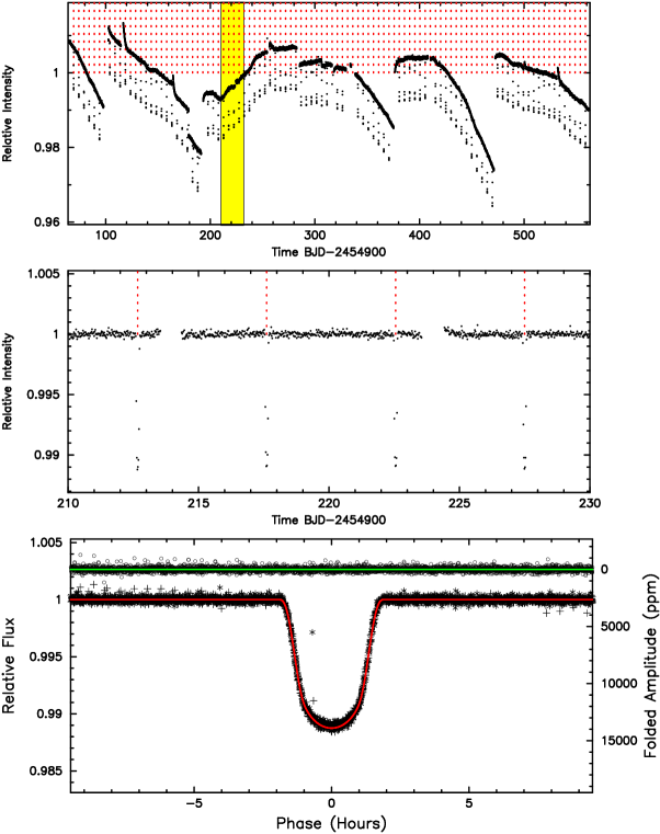
Figure 1: The Kepler light curve of Kepler-15. The top panel displays the Q1 to Q6 time series photometry. The long-term trends are primarily caused by focus changes in the telescope and by transitions to different detectors (due to spacecraft rotation). The (red) vertical dotted lines mark the location of the transits. The middle panel shows a close-up of the (yellow) rectangle in the upper panel (with trends removed), and the bottom panel contains the data phased to the transit period of 4.943 days. We also show the light curve at opposite phase slightly above the transit light curve. It shows no sign of a secondary eclipse.

Kepler-15 was already identified as a planet candidate in the 35 days of the first quarter (Q1) of Kepler photometry and was assigned the Kepler-Object-of-Interest (KOI) identifier KOI-128. The target star has a Kepler magnitude (K_p) of 13.76. Processing of the photometry was carried out using the standard Kepler pipeline (Jenkins et al. 2010a). The data were sampled at the typical 30 minute “long cadence”. Figure 1 displays the Kepler light curve for Kepler-15. The top panel shows the Photometric Analysis (PA) light curve for Q1 through Q6. The middle panel displays a small segment of these data that have been processed by the Presearch Data Conditioning (PDC) software to remove spacecraft data artifacts. The lower panel shows the data phased to the candidate period of $4.943$ days. The transit has a duration of 3.5 hours and a photometric depth of 12.3  mmag (1.2$\%$). The period of the transit is $4.9427813\pm 0.000002$ days.

The radius of the star is estimated in the Kepler Input Catalog (KIC) as $1.4$ R_⊙. Such a large stellar radius yields a rather large radius for the companion of $\approx 1.5$ R_Jup. This large planetary radius prompted our ground-based follow-up campaign to confirm and characterize this system. If such a large radius for the planet were confirmed, the planet would most-likely belong to the family of inflated hot Jupiters, with a very low mean density, similar to Kepler-7b (Latham et al. 2010).

2.1 Difference Image Analysis

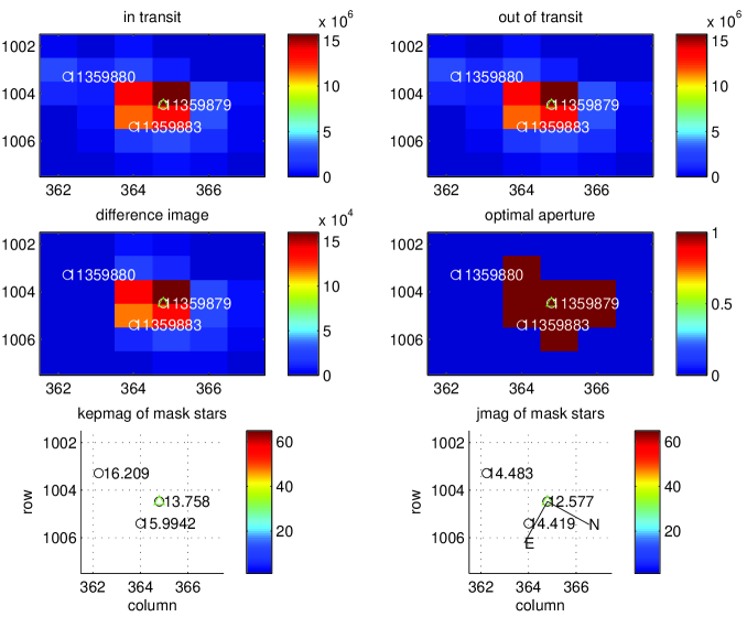
Figure 2: Difference images for Kepler-15 (KIC 11359879). Each panel shows the same section of the CCD (x-axis is the pixel column and y-axis is the pixel row). One Kepler pixel is 3.96 arcsec². The color coding represents the flux level in each pixel. The top two panels display the in- and out of transit images and the difference image is shown in the middle left panel. The optimal aperture for the photometry can be seen for comparison in the middle right panel. The lower two panels show the field, its orientation on the chip, and the K_p and J-band magnitudes of nearby KIC stars.

To eliminate the possibility that the transit signatures are due to transits on a background star, the change in centroid location during transit was examined using the difference image method described in Torres et al. (2011). This method fits the measured Kepler Pixel Response Function (PRF) to a difference image formed from the average in-transit and average out-of-transit pixel images. This difference image method has the advantage of directly measuring the location of the transiting signal. In addition, the PRF is fit to the out-of-transit image to measure the position of the target star. An example of the average images including the optimal aperture pixels used to create the light curve and the local stellar scene is shown in Fig 2. The difference image completely rules out that the transits occur on the second star in the aperture (KIC 11359883). A transit on KIC 11359883 would appear in the difference image as a star centered on the pixel containing KIC 11359883.

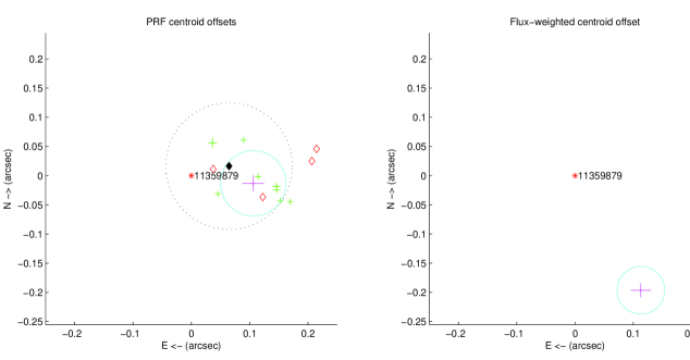
Figure 3: Pixel Response Function (PRF) centroid offset (left panel) and flux-weighted centroid offset (right panel) for Kepler-15 (KIC 11359879). The observed centroid is displayed as large cross with a solid circle showing the 3-sigma uncertainty. The left panel also contains the individually observed PSF centroids for Q1 through Q7 (small crosses) as well as the centroid results from our test (see text for details) to estimate the effect of crowding (small diamonds). A systematic offset to the west of 0.1 arcsecs due to crowding is observed and reproduced by the test results.

These centroids are then subtracted to provide the offset of the transit signal location from the target star. The offsets from Q1 through Q8 are shown as the green crosses in the left panel of Fig. 3, where the arms of the green crosses show the uncertainty in RA and DEC. We see that in all quarters the transit signal location is consistently offset to the west by about 0.1 arcsec. The robust average across quarters, weighted by the quarterly uncertainty, is shown by the magenta cross, with the solid circle giving its 3-sigma uncertainty radius. This average centroid observation is offset by about 0.1 arcsec with a significance of 5.7 sigma. The right panel of Fig. 3 shows the transit signal source estimated by correlating the transit model with observed photocenter motion (Jenkins et al. 2011b). Photocenter motion also shows a statistically significant (17 sigma) transit signal location offset, but the offsets from the two methods are in significant disagreement, suggesting that these offsets are due to measurement bias.

The uncertainty in PRF-fit centroids is based on the propagation of pixel-level uncertainty and does not include a possible PRF fit bias. Sources of PRF fit bias include scene crowding, because the fit is of a single PRF assuming a single star, as well as PRF error. The measured offset is the difference between the centroids of the difference and out-of-transit images, so common biases such as PRF error should cancel. Bias due to crowding, however, will not cancel because, to the extent that variations in other field stars are not correlated with transits, field stars will not contribute to the difference image. In other words the difference image will have the appearance of a single star where the transit occurs, so there is no crowding bias in the difference image PRF fit.

To investigate the possibility that the observed offsets are due to PRF-fit bias caused by crowding we modeled the local scene using stars from the Kepler Input Catalog supplemented by UKIRT observations (see section 3.2) and the measured PRF, induced the transit on Kepler-15 in the model, and performed the above PRF fit analysis on the model difference and out-of-transit images. The resulting model offsets for quarters one through four is shown on Figure  3 as open diamonds. (Only four quarters are shown because the model is very nearly periodic with a period of one year.) The robust average of the model offsets, again weighted by propagated uncertainty, is shown as the filled diamond, with the dotted circle showing the average model 3-sigma uncertainty. We see that the model points are consistently offset to the west, and the observed average is well-contained within the model 3-sigma uncertainty. This is consistent with the observed in-transit centroid offsets being due to PRF fit bias (mostly) due to crowding. We therefore can be highly confident that the transit signal is due to transits on Kepler-15.

3 Confirmation by ground-based follow-up observations

3.1 Reconnaissance Spectroscopy

As part of the Kepler Follow-up Observing Program (FOP) strategy, we first obtained two reconnaissance spectra of Kepler-15 with the Tull Coudé Spectrograph (Tull et al. 1995) at the Harlan J. Smith 2.7 m Telescope at McDonald Observatory. A comparison with a library of stellar templates yielded the following stellar parameters: T${}_{\rm eff}=5500$ K, log g = 4.0 (first spectrum), log g = 4.5 (second spectrum) and v$\sin i$ = 2 km s^-1. The absolute RV of Kepler-15 is $-20$ km s^-1 and the two measurements differ by less than $1$ km s^-1 (which is within the measurement uncertainty) between the two visits (which were separated by one month). These results exclude the scenario where a grazing eclipsing binary produces a false-alarm (a binary would have produced a significant RV shift between the two reconnaissance spectra).

3.2 Imaging

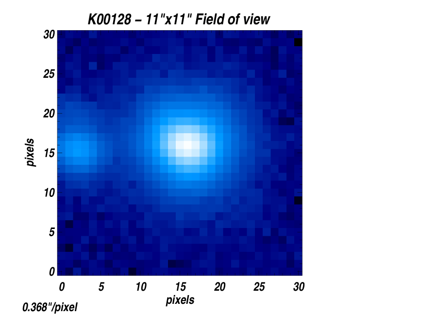
Figure 4: I-band image of the field centered on Kepler-15 (KOI-128) taken with the 1 m telescope at Lick Observatory. The scale is $11\times 11$ arcseconds, north is up and east is left. KIC 11359883, the other KIC star is the Kepler-15 aperture, is visible 4 arcseconds to the east.

A seeing limited image of the field around Kepler-15 was obtained at Lick Observatory’s 1 m Nickel telescope using the Direct Imaging Camera. A single one-minute exposure was taken in the I-band (7500-10500 Å), resulting in an image with seeing of approximately 1.5 arcseconds. Observations occurred under clear skies and new moon during an observing run in 2010 July 8-10. The I-band image is shown in Figure 4. With the exception of the nearby star KIC 11359883 (K${}_{\rm p}=15.99$), no other object is detected inside the optimal aperture of Kepler-15.

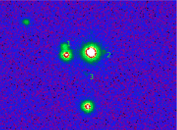
Figure 5: J-band image of the field around on Kepler-15 (center) taken with UKIRT. North is up and east is left. The scale is $\sim 25\times 40$ arcsecs. We detect three additional objects located within the optimal aperture of Kepler-15 (besides KIC 11359883). Object nr.1 and 2 are real, but nr.3 is an artifact. The two other stars seen in this image to the far east and south are located outside the optimal aperture.

A deep J-band image of the field was obtained at UKIRT (see Figure 5). Three additional objects that are located within the optimal aperture are detected in the UKIRT image. Object Nr.1 is a star close to KIC 11359883 and estimated to have K${}_{\rm p}=19.4\pm 0.6$. Object Nr.2 is very close to Kepler-15 and we estimate K${}_{\rm p}=21.4\pm 0.9$ . Object Nr. 3 is an artifact caused by electronic cross-talk. We estimate the K_p values from the measured J-band magnitudes and the typical K_p-J color according to the Besancon synthetic Galactic population model (Robin et al. 2003) for stars of this J magnitude at this place on the sky. Object Nr.1 is also barely visible in the wings of the PSF of KIC 11359883 in the Lick I-band image.

We have also obtained speckle observations at the WIYN 3.5-m telescope located on Kitt Peak. The observations make use of the Differential Speckle Survey Instrument (DSSI), a recently upgraded speckle camera described in Horch et al. (2010) and Howell et al., (2011). The DSSI provides simultaneous observations in two filters by employing a dichroic beam splitter and two identical EMCCDs as the imagers. We observed Kepler-15 simultaneously in ”V” and ”R” bandpasses where ”V” has a central wavelength of 5620 Å, and ”R” has a central wavelength of 6920 Å, and each filter has a FWHM=400 Å. The details of how we obtain, reduce, and analyze the speckle results and specifics about how they are used to eliminate false positives and aid in transit detection are described in Howell et al. (2011).

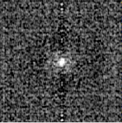
Figure 6: Reconstructed R-band speckle image of Kepler-15 taken with the WIYN telescope at Kitt Peak. No additional stars are detected within the annulus from 0.05 to 1.8 arcsec to a limit of (5$\sigma$) 3.52 magnitudes fainter than the target star. The image is $2.8\times 2.8$ arcsecs.

The speckle observations of the Kepler-15 were obtained on 2010 October 24 (UT) and consisted of five sets of 1000, 40 msec individual speckle images. Our R-band reconstructed image is shown in Figure 6 with details of the image composition described in Howell et al. (2011). Along with a nearly identical V-band reconstructed image, the speckle results reveal no companion star near Kepler-15 within the annulus from 0.05 to 1.8 arcsec to a limit of (5$\sigma$) 3.52 magnitudes fainter in R and 3.16 magnitudes fainter in V relative to the K${}_{\rm p}=13.76$ target star.

As a result of the direct imaging of the field around Kepler-15 we found that two additional stars (besides KIC 11359883) are located within the optimal aperture of Kepler-15. However, both stars are fainter than K${}_{\rm p}=19$ and have a negligible effect on the photometry. Only KIC 11359883 (K${}_{\rm p}=15.99$) has a significant effect and we take the diluting effect of its light contribution into account for the light curve modeling.

3.3 Precise Radial Velocity Measurements

We performed precise RV follow-up observations of Kepler-15 with the HET (Ramsey et al. 1998) and its HRS spectrograph (Tull 1998). The queue-scheduled observing mode of the HET usually leads to the situation that on a given night, data for many different projects and with different instruments are obtained. The observations are ranked according to priorities distributed by the HET time-allocation-committees as well as additional timing constraints. We entered Kepler-15 into the HET queue to be observed in a quasi-random fashion with a cadence of a few days to allow proper sampling of the suspected 4.9 d RV orbit. We observed this target from 2010 March 29 until 2010 November 9. We collected 24 HRS spectra with the I₂-cell in the light path for precise RV measurements. Furthermore, we obtained one spectrum without the I₂-cell to serve as a stellar “template” for the RV computation and to better characterize the properties of the host star.

Because of the faintness of this star, the HRS setup we employed for the RV observations is slightly different from our standard planet search RV reduction pipeline (described in detail in Cochran et al. 2004). We used the 2 arcsec fiber to feed the light into the HRS. The cross-disperser setting was “600g5822”, which corresponds to a wavelength coverage from 4814 to 6793 Å, thus covering the entire I₂ spectral range of 5000-6400 Å. We also used a wider slit to gain a higher throughput for this faint target, reducing the spectral resolving power to $R=\lambda/\Delta\lambda=30,\!000$ (instead of our nominal $R=60,\!000$). Moreover, two sky fibers allow us to simultaneously record the sky background and to properly subtract it from our data. The CCD was binned 2x2, which yields 4 pixels per resolution element. This new setup is better suited for observations of the faint Kepler targets. The exposure time for each observation was $1200$ seconds. The mean S/N-ratio of the 24 spectra is $42\pm 6$ per resolution element. As higher spectral resolution is advantageous for the template spectrum, we obtained this spectrum with $R=60,\!000$ and a longer exposure time of 2700 seconds. We computed precise differential RVs with our Austral I₂-cell data modeling algorithm (Endl et al. 2000). The HET/HRS RV data are listed in table 1. The data have an overall rms-scatter of $60~{}{\rm m\,s}^{-1}$ and average internal errors of $25\pm 8~{}{\rm m\,s}^{-1}$.

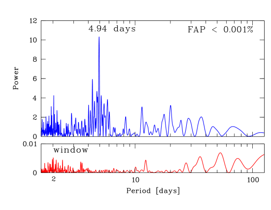
Figure 7: Lomb-Scargle periodogram of the HET/HRS RV results for Kepler-15. The top panel shows the power spectrum of the periodogram with a highly significant peak (false-alarm probability FAP $<10^{-5}$) at the transit period of 4.94 days. The lower panel displays the window function of the HET observations.

We performed a period search in our HET RV data set using the classic Lomb-Scargle periodogram (Lomb 1976, Scargle 1982). Fig. 7 displays the power spectrum over the period range from 2 to 100 days. The highest peak is located at a period of $4.94$  days. This is an independent confirmation of the transit period. The signal is also statistically highly significant, we estimate a false-alarm-probability (FAP) of less than $10^{-5}$ using a bootstrap randomization scheme (Kürster et al. 1997).

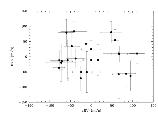
Figure 8: Correlation between the bisector velocity span (BVS) and the RV measurements of the 24 HET spectra. No correlation is detected (linear correlation coefficient is $-0.076$).

We have also determined line bisectors from the HET spectra. As we could use only the small fraction of the available spectral range that lies outside the I₂ region ($5000-6400$ Å) the uncertainties in the bisector velocity span (BVS) are quite large, the average error of the BVS measurements is $43\pm 17$ m s^-1 and they have a total rms-scatter of 46 m s^-1. The bisector measurements are given in table 2. Figure 8 shows the correlation plot of BVS values versus RV measurements. The linear correlation coefficient is $-0.076$ corresponds to a 72% probability that the null-hypothesis of zero correlation is true. This further strengthens the case that the RV modulation is due to an orbiting companion.

We have also taken 6 spectra between 2010 July and August using the FIbre–fed Échelle Spectrograph (FIES) at the 2.5 m Nordic Optical Telescope (NOT) at La Palma, Spain (Djupvik & Andersen 2010). We used the medium and the high–resolution fibers ($1\farcs 3$ projected diameter) with resolving powers of $R\approx 46,\!000$ and $67,\!000$, respectively, giving a wavelength coverage of $\sim 3600-7400$ Å. We used the wavelength range from approximately $\sim 4100-5600$ Åto determine the RVs following the procedures described in Buchhave et al. (2010). The exposure time was between 2400 and 3600 seconds, yielding a S/N from 22 to 30 per pixel in the wavelength range used. The FIES RV results are also given in Table 1.

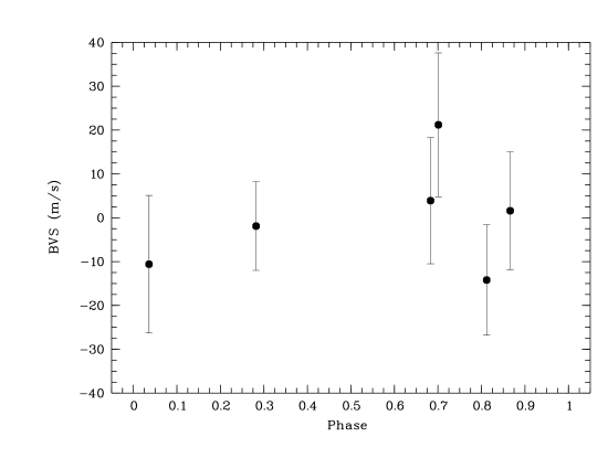
Figure 9: FIES line bisectors and their uncertainties as a function of transit/orbital phase of Kepler-15. We detect no significant variability.

We also determined the line bisectors for the 6 FIES spectra. They have a higher precision than the HRS results since we could use the entire spectrum for the analysis (FIES does not use an I₂-cell). The FIES bisector data are listed in table 2 and shown as a function of orbital phase in Figure 9. The average uncertainty of the FIES bisector measurements is $13.8\pm 2.3$ m s^-1 and their total scatter is $12.5$ m s^-1. They appear to be constant within the measurement uncertainties.

4 Results

4.1 Host star characterization

We determined stellar parameters using the local thermodynamic equilibrium (LTE) line analysis and spectral synthesis code MOOG (Sneden 1973), together with a grid of Kurucz (1993) ATLAS9 model atmospheres. The method used is virtually identical to that described in Brugamyer et al. (2011). To check this method, we first measured the equivalent widths of a carefully selected list of 48 neutral iron lines and 11 singly-ionized iron lines in a spectrum of the daytime sky, taken using the same instrumental setup and configuration as that used for Kepler-15. MOOG force-fits abundances to match these measured equivalent widths, using declared atomic line parameters. By assuming excitation equilibrium, we constrained the stellar temperature by eliminating any trends with excitation potential; assuming ionization equilibrium, we constrained the stellar surface gravity by forcing the derived iron abundance using neutral lines to match that of singly-ionized lines. The microturbulent velocity was constrained by eliminating any trend with reduced equivalent width (=EW/$\lambda$). Our derived stellar parameters for the Sun (using our daytime sky spectrum) are as follows: T_eff = $5755\pm 70$ K, log g = $4.48\pm 0.09$ dex, Vmic = $1.07\pm 0.06$ km s^-1, and log $\epsilon$ (Fe) = $7.53\pm 0.05$ dex.

The process described above was repeated for the HET/HRS spectrum taken without the I₂ cell of Kepler-15. We took the difference, on a line-by-line basis, of the derived iron abundance from each line. Our quoted iron abundance is therefore differential with respect to the Sun. To estimate the rotational velocity of the star, we synthesized three 5-Å-wide spectral regions in the range 5640 - 5690 Å, and adjusted the gaussian and rotational broadening parameters until the best fit (by eye) was found to the observed spectrum. The results of our analysis yield the following stellar parameters for Kepler-15: T_eff = $5595\pm 120$ K, log g $=4.23\pm 0.2$, Vmic = $1.09\pm 0.1$ km/s, [Fe/H] = $+0.36\pm 0.07$, and Vrot = $2\pm 2$ km s^-1. The preliminary results from the reconnaissance spectroscopy (T${}_{\rm eff}\approx 5500$ K, log g $=4.0$ & $4.5$ and Vrot = $2$ km s^-1) compare very well with this improved spectroscopic analysis.

4.2 Orbital Solution and Planet Parameters

We used a Markov Chain Monte Carlo (MCMC) algorithm to perform a simultaneous fit to the light curve and the RV results. This analysis was performed using the 24 HET RV measurements and the Q1 through Q6 Kepler photometry. The model fits for $\rho_{\star}$, T0, Period, b, r/R_⋆, $e\sin\omega$, $e\cos\omega$, $\gamma$, and the photometric zeropoint. The transit shape is characterized by the Mandel-Agol analytic derivations (Mandel & Algol 2002) and the planetary orbit is assumed to be Keplerian. The best fit model is computed by simultaneously fitting radial velocity measurements and Kepler photometry and then minimizing the chi-square statistic with a Levenberg-Marquart method. To obtain probability distributions, the best fit model is used to seed a MCMC computation. Our MCMC algorithm employs a hybrid sampler based on Gregory (2011) that uses a Gibb-sampler or a buffer of previously computed chain points to generate proposals to jump to new locations in parameter space. The addition of the buffer allows for a calculation of vectorized jumps that allow for efficient sampling of highly correlated parameter space. The MCMC distributions are shown in Figure 11.

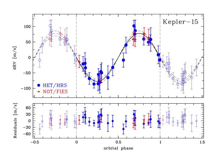
Figure 10: HET/HRS (circles) and NOT/FIES (triangles) RV data and the best-fit orbital solution (solid line) phased to the transit period of 4.94 days (top panel). The semi-amplitude $K$ is $78.7\pm 9.1$ m s^-1 corresponding to a mass of $0.66\pm 0.08$ M_Jup for the planetary companion. The bottom panel shows the residuals: the 24 HRS points have a residual rms scatter of 16.9 m s^-1 and the 6 FIES points have a residual rms scatter of 9.6 m s^-1. (The data are repeated for a second cycle.)

The results of this MCMC modeling are summarized in Table 3. For all parameters we list the median values along with their 68% uncertainty interval ($\pm 1\sigma$) based on the MCMC distributions. The transit ephemeris is $T0=69.328651^{+0.000084}_{-0.000096}$ (BJD-2454900) and the period is $P=4.942782\pm 0.0000013$ days. The transit has a depth of $11127.7^{+12.8}_{-14.4}$ ppm. Taking into account the diluting effect of the other star in the aperture ($97.0\pm 0.003$% of the light in the aperture comes from Kepler-15) we find a radius ratio of $R_{\rm planet}/R_{*}=0.09960^{+0.00055}_{-0.00053}$. The RV semi-amplitude $K$ is $78.7^{+8.5}_{-9.1}$ m s^-1. The orbital eccentricity was allowed as a free parameter during the modeling process, but we find no strong indication for an eccentric orbit ($e\sin\omega=-0.123^{+0.089}_{-0.110},e\cos\omega=0.053^{+0.086}_{-0.079}$). Figure  10 displays the HET/HRS and the NOT/FIES results compared to the RV orbit (assuming $e=0$). The reduced $\chi^{2}$ of this fit is 0.52, indicating that our RV error bars are slightly overestimated. The residual rms-scatter for the two RV data set is: 16.9 m s^-1 for the HET/HRS data and 9.6 m s^-1 for the NOT/FIES data.

The distribution of $\rho_{\star}$ from the model fit above and T_eff and [Fe/H] from the spectroscopic determination are used together to match Yonsei-Yale (Y²) models (Yi et al. 2001). This is known as the “$\rho_{\star}$ method” (see e.g. Sozetti et al. 2007, Brown 2010). The probability distributions of the matching stellar parameters, M_⋆, R_⋆, age, luminosity are also shown in Figure 11. From isochrone fitting we derive a mass for the star of $1.018^{+0.044}_{-0.052}$ M_⊙, a radius of $0.992^{+0.058}_{-0.070}$ R_⊙ and an age of $3.7^{+3.5}_{-1.6}$ Gyrs. The log  g from the isochrone fit is $4.46^{+0.053}_{-0.050}$, 0.2 dex higher than the spectroscopically derived log g value of $4.23\pm 0.2$. A systematic difference in log g values for high metallicity stars has been discussed previously for Kepler-6 (Dunham et al. 2010). We note that the difference in our case is the opposite (the spectroscopic log g is lower, for Kepler-6 it was higher by 0.35 dex). However, the error bars of both methods still overlap for Kepler-15. All stellar parameters from the isochrone fit are also listed in Table 3.

The planetary orbit and parameters are derived by using the Markov chains from the model and isochrone fits. Random chains are selected from each fit to calculate the planet mass, radius, semi-major axis, a/R_⋆ and presented in Figure 11 and Table 3.

5 Discussion

After passing all tests and observational diagnostics, from photometric centroid shifts to spectroscopic line bisectors, and the fact that an RV orbit in period and phase with the transit ephemeris is detected, we conclude that Kepler-15b is indeed a new transiting planet. All our currently available data suggest a planet with a mass of $0.66$ M_Jup, a radius of 0.96 R_Jup and a mean density of $0.9\pm 0.2$ g cm^-3 orbiting a metal-rich ([Fe/H]=0.36) G-type star every 4.94 days. Kepler-15 is tied with Kepler-6 as the most metal-rich host star of all currently published Kepler planets.

Although we initially suspected a large planetary radius, our results demonstrate rather the opposite. Figure 12 shows that the planet’s radius is modestly smaller than planets of similar mass and irradiation level. This suggests that the planet is more enriched in heavy elements than most other transiting planets. Given the high stellar metallicity, and the connection between stellar metallicity and planetary heavy elements (Guillot et al. 2006, Burrows et al. 2007, Miller & Fortney 2011), this is is not surprising. Using the tables of Fortney et al. (2007), we estimate a heavy element mass within the planet of at least 30-40 Earth masses.

6 Summary & Outlook

We report the discovery of Kepler-15b, a hot Jupiter ($P=4.94$ d) that is enriched in heavy elements ($\approx 20\%$ in mass) in orbit around a metal-rich G-type star with K_p=13.76. Kepler-15b is the first giant planet from the Kepler mission that we confirmed with the HET, demonstrating the capability of this facility as an integral part of the ground-based spectroscopic follow-up effort of the Kepler mission. In 2010 we spent a total of 65 hours on the Kepler field and collected data for 11 Kepler candidates. Besides the planet presented here, we have confirmed several other giant planets around Kepler stars, e.g. Kepler-17b (Désert et al. 2011). The remaining HET planet confirmations will be included in a catalog of Kepler giant planets (Caldwell et al. in prep.).

The HET will obtain a major upgrade to its secondary tracker assembly to allow a wider field of view. This upgrade will start in fall 2011. During the telescope downtime the HRS will also undergo a major upgrade, including more efficient optics and fibers, as well as image slicers, to boost the overall throughput by several factors. Once the HET is back on sky in early 2012, these improvements should allow us to use the HET/HRS also for the confirmation and validation of low mass Kepler planet candidates in the Neptune and Super-Earth range, similar to Kepler-10b (Batalha et al. 2011).

Figure 11: Markov chain Monte Carlo distributions for the model parameters for the Kepler-15 system. The resulting values and uncertainties of the system parameters are listed in Table 3. For the period value we plot the difference to P0=4.942782 days.

Figure 12: Planet mass vs. radius for a collection of transiting planets with masses from 0.3 to 1.0 M_Jup. Values are taken from: http://www.inscience.ch/transits/. Kepler-15 is shown as a filled circle. The solid curve is for a 1 M_Jup model planet at 4.5 Gyr (Miller, Fortney, and Jackson, 2009). While many planets are inflated relative to this curve, Kepler-15 is clearly below it. While a radius-inflation mechanism could still be at work in this planet, the small radius indicates that the planet is rich in heavy elements.

Table 1: Radial velocity measurements for Kepler-15

BJD [d]	dRV[m s-1]	err[m s-1]	Telescope
2455284.981307	57.6	9.5	HET
2455286.970962	-46.7	19.1	HET
2455335.858420	-59.8	18.8	HET
2455337.868951	-0.3	23.1	HET
2455346.841507	-56.9	38.0	HET
2455349.813386	16.9	29.0	HET
2455357.791818	48.4	25.7	HET
2455359.784683	0.1	21.3	HET
2455363.784770	67.8	19.3	HET
2455370.733856	-77.6	13.1	HET
2455395.690132	-76.7	22.7	HET
2455397.881162	94.8	34.5	HET
2455399.884842	-25.2	29.2	HET
2455405.675158	-72.3	35.0	HET
2455470.693433	-24.0	27.0	HET
2455494.620347	-70.9	25.9	HET
2455497.633684	66.4	15.1	HET
2455498.603079	-12.6	23.8	HET
2455501.603733	110.5	18.0	HET
2455502.592532	66.4	37.9	HET
2455504.595288	-37.6	22.9	HET
2455506.589121	84.1	22.7	HET
2455508.600869	-10.9	34.0	HET
2455509.575509	-41.4	31.9	HET
2455378.649338	148.5	19.0	NOT
2455384.700553	58.0	20.1	NOT
2455423.403627	136.4	26.2	NOT
2455425.457207	0.0	19.0	NOT
2455427.440796	130.9	20.8	NOT
2455432.470155	130.7	24.5	NOT

Table 2: Bisector measurements for Kepler-15

BJD [d]	bisector[m s-1]	bserr[m s-1]	Spectrograph
2455284.981307	54.0	35.4	HRS
2455286.970962	34.2	48.2	HRS
2455335.858420	79.1	43.4	HRS
2455337.868951	24.4	29.3	HRS
2455346.841507	-11.4	66.6	HRS
2455349.813386	-10.9	51.4	HRS
2455357.791818	80.3	36.0	HRS
2455359.784683	-11.3	43.1	HRS
2455363.784770	8.5	26.4	HRS
2455370.733856	-36.4	26.9	HRS
2455395.690132	-12.5	33.9	HRS
2455397.881162	-63.3	50.0	HRS
2455399.884842	-71.2	39.6	HRS
2455405.675158	-19.9	62.2	HRS
2455470.693433	-50.5	35.2	HRS
2455494.620347	-15.1	26.4	HRS
2455497.633684	-58.0	79.6	HRS
2455498.603079	42.5	76.9	HRS
2455501.603733	10.3	33.6	HRS
2455502.592532	10.6	18.6	HRS
2455504.595288	-6.2	31.2	HRS
2455506.589121	-55.9	41.3	HRS
2455508.600869	-50.6	67.4	HRS
2455509.575509	83.1	31.4	HRS
2455378.649338	-14.2	12.6	FIES
2455384.700553	-10.6	15.7	FIES
2455423.403627	1.6	13.4	FIES
2455425.457207	-1.9	10.1	FIES
2455427.440796	3.9	14.4	FIES
2455432.470155	21.2	16.4	FIES

Table 3: Parameters of the Kepler-15 transiting system

Parameter [unit]	value	+1$\sigma$	-1$\sigma$	notes
KIC	11359879
KOI	128
Kp[mag]	13.76
RV [km s-1]	-20.0	+1.0	-1.0
Period [days]	4.942782	+0.0000013	-0.0000013
T0 [BJD]	2454969.328651	+0.000084	-0.000096
$\rho_{\star}$ [g cm-3]	1.47	+0.26	-0.28
b	0.554	+0.023	-0.024
Rplanet / R⋆	0.0996	+0.00055	-0.00053
i [deg]	87.44	+0.18	-0.20
a/R⋆	12.8	+1.2	-1.5
M⋆ [M⊙]	1.018	+0.044	-0.052	(isochrone fit)
R⋆ [R⊙]	0.992	+0.058	-0.070	(isochrone fit)
Age [Gyr]	3.7	+1.5	-3.6	(isochrone fit)
Teff [K]	5515	+122	-130	(isochrone fit)
Teff [K]	5595	+120	-120	(spectroscopic fit)
log L/L⊙	-0.087	+0.078	-0.088	(isochrone fit)
log g [cgs]	4.46	+0.053	-0.050	(isochrone fit)
log g [cgs]	4.23	+0.2	-0.2	(spectroscopic fit)
$\rm{[Fe/H]}$	0.36	+0.07	-0.07	(spectroscopic fit)
Vrot [km s-1]	2.0	+2.0	-2.0	(spectroscopic fit)
Rplanet [$R_{\oplus}$]	10.8	+0.63	-0.77
Rplanet [$R_{\rm Jup}$]	0.96	+0.06	-0.07
K [m s-1]	78.7	+8.5	-9.5
$e\sin\omega$	-0.123	+0.089	-0.110
$e\cos\omega$	0.053	+0.086	-0.079
Mplanet [$M_{\oplus}$]	209	+24	-28
Mplanet [$M_{\rm Jup}$]	0.66	+0.08	-0.09
a [AU]	0.05714	+0.00086	-0.00093
$\rho_{\rm planet}$ [g cm-3]	0.93	+0.18	-0.22

References

- (1) Batalha, N., Borucki, W., Bryson, S., et al. 2011, ApJ, 729, 27
- (2) Brown, T. M. 2010, ApJ, 709, 535
- (3) Buchhave, L. A., Bakos, G. A., Hartman, J. D. et al. 2010, ApJ, 720, 1118
- (4) Borucki, W. J., et al. 2010, Science, 327, 977
- (5) Borucki, W. J., Koch, D. J., Basri, G. et al. 2011, ApJ, in press
- (6) Brugamyer, E., Dodson-Robinson, S. E., Cochran, W. D., Sneden, C. 2011, ApJ, submitted
- (7) Burrows, A., Hubeny, I., Budaj, J., Hubbard, W. B. 2007, ApJ, 661, 502
- Djupvik & Andersen (2010) Djupvik, A. A., & Andersen, J. 2010, in “Highlights of Spanish Astrophysics V” eds. J. M. Diego, L. J. Goicoechea, J. I. González-Serrano, & J. Gorgas (Springer: Berlin), p. 211
- (9) Désert, J.-M., Charbonneau, D., Demory, B.-O. et al., ApJ, in prep.
- (10) Dunham, E. W., Borucki, W. J., Koch, D. G., Batalha, N. M., Buchhave, L. A., et al. 2010, ApJ, 713, L136
- (11) Endl, M., Kürster, M., & Els, S. 2000, A&A, 362, 585
- (12) Fortney, J. J., Marley, M. S., & Barnes, J. W. 2007, ApJ, 659, 1661
- (13) Gregory, P. C. 2011, MNRAS, 410, 94
- (14) Guillot, T., Santos, N. C., Pont, F. et al. 2006, A&A, 453, L21
- (15) Horch, E. P. et al., 2010, AJ, 141, 45
- (16) Howell, S. B., et al., 2011, AJ, 142, 19
- (17) Jenkins, J. M., Caldwell, D. A., Chandrasekaran, H., et al. 2010a, ApJ, 713, L87
- (18) Jenkins, J. M., Borucki, W. J., Koch, D. G., et al. 2010b, ApJ, 724, 1108
- (19) Kürster, M., Schmitt, J. H. M. M., Cutispoto, G., & Dennerl, K. 1997, A&A, 320, 831
- (20) Kurucz, R. 1993, ATLAS9 Stellar Atmosphere Programs and 2 km/s grid. Kurucz CD-ROM No. 13. (Cambridge: Smithsonian Astrophys. Obs.)
- (21) Latham, D. W., Borucki, W. J., Koch, D. G., et al. 2010, ApJ, 713, L140
- (22) Lomb, N. R. 1976, Ap&SS, 39, 447
- (23) Mandel, K. & Algol, E. 2002, ApJ, 580, L171
- (24) Miller, N., Fortney, J. J., & Jackson, B. 2009, ApJ, 702, 1413
- (25) Miller, N., & Fortney, J. J. 2011, ApJ, accepted
- (26) Scargle, J. D. 1982, ApJ, 263, 835
- (27) Sneden, C. A. 1973, Ph.D. thesis, Univ. of Texas at Austin
- (28) Sozetti, A., Torres, G., Charbonneau, D., Latham, D., Holman, M. J., Winn, J. N., Laird, J. B., O’Donovan, F. T. 2007, ApJ, 664, 1190
- (29) Ramsey, L. W., et al. 1998, Proc. SPIE, 3352, 34
- (30) Robin, A. C., Reylé, C., Derriére, S., Picaud, S. 2003, A&A, 409, 523
- Torres et al. (2011) Torres, G. et al. 2011, ApJ, 727, 24
- (32) Tull, R. G., MacQueen, P. J., Sneden, C., Lambert, D. L. 1995, PASP, 107, 251
- (33) Tull, R. G. 1998, Proc. Soc. Photo-opt. Inst. Eng., 3355, 387
- (34) Yi, S., Demarque, P., Kim, Y.-C., Lee, Y.-W., Ree, C. H., Lejeune, T., & Barnes, S. 2001, ApJS, 136, 417