Distributed Flames in Type Ia Supernovae

Abstract

At a density near a few $\times 10^{7}$ g cm^-3, the subsonic burning in a Type Ia supernova enters the distributed regime (high Karlovitz number). In this regime, turbulence disrupts the internal structure of the flame, and so the idea of laminar burning propagated by conduction is no longer valid. The nature of the burning in this distributed regime depends on the turbulent Damköhler number ($\mathrm{Da}_{T}$), which steadily declines from much greater than one to less that one as the density decreases to a few $\times 10^{6}$ g cm^-3. Classical scaling arguments predict that the turbulent flame speed $s_{T}$, normalized by the turbulent intensity $\check{u}$, follows $s_{T}/\check{u}=\mathrm{Da}_{T}^{1/2}$ for $\mathrm{Da}_{T}\lower 0.43057pt\hbox{\hbox to0.0pt{\raise 2.58334pt\hbox{\hskip 1.29167pt{{$\scriptscriptstyle<$}}}\hss} \kern-1.72218pt{{$\scriptscriptstyle\sim$}}}1$. The flame in this regime is a single turbulently-broadened structure that moves at a steady speed, and has a width larger than the integral scale of the turbulence. The scaling is predicted to break down at $\mathrm{Da}_{T}\approx 1$, and the flame burns as a turbulently-broadened effective unity Lewis number flame. This flame burns locally with speed $s_{\lambda}$ and width $l_{\lambda}$, and we refer to this kind of flame as a $\lambda$-flame. The burning becomes a collection of $\lambda$-flames spread over a region approximately the size of the integral scale. While the total burning rate continues to have a well-defined average, $s_{T}\sim\check{u}$, the burning is unsteady. We present a theoretical framework, supported by both 1D and 3D numerical simulations, for the burning in these two regimes. Our results indicate that the average value of $s_{T}$ can actually be roughly twice $\check{u}$ for $\mathrm{Da}_{T}\lower 0.43057pt\hbox{\hbox to0.0pt{\raise 2.58334pt\hbox{\hskip 1.29167pt{{$\scriptscriptstyle>$}}}\hss} \kern-1.72218pt{{$\scriptscriptstyle\sim$}}}1$, and that localized excursions to as much as five times $\check{u}$ can occur. We also explore the properties of the individual flames, which could be sites for a transition to detonation when $\mathrm{Da}_{T}\sim 1$. The $\lambda$-flame speed and width can be predicted based on the turbulence in the star (specifically the energy dissipation rate $\varepsilon^{*}$) and the turbulent nuclear burning time scale of the fuel $\tau_{\mathrm{nuc}}^{T}$. We propose a practical method for measuring $s_{\lambda}$ and $l_{\lambda}$ based on the scaling relations and small-scale computationally-inexpensive simulations. This suggests that a simple turbulent flame model can be easily constructed suitable for large-scale distributed supernovae flames. These results will be useful both for characterizing the deflagration speed in larger full-star simulations, where the flame cannot be resolved, and for predicting when detonation occurs.

1 INTRODUCTION

In Aspden et al. (2008a) (henceforth Paper I) three-dimensional simulations of resolved flames were performed that examined the interactions between turbulence and a carbon-burning flame in a Type Ia supernova at different densities. Because of the strong dependence of flame width and speed on density, this study can be viewed as a survey of the behavior of the flame at variable Karlovitz number,

$$\mathrm{Ka}=\sqrt{\frac{\check{u}^{3}}{s_{L}^{3}}\frac{l_{L}}{l}}.$$ (1)

Here $s_{L}$ and $l_{L}$ are the laminar flame speed and width, respectively, and $\check{u}$ and $l$ are the turbulent intensity (rms velocity) and integral length scale (defined conventionally as the integral of the longitudinal correlation function). For $\mathrm{Ka}\lower 0.43057pt\hbox{\hbox to0.0pt{\raise 2.58334pt\hbox{\hskip 1.29167pt{{$\scriptscriptstyle<$}}}\hss} \kern-1.72218pt{{$\scriptscriptstyle\sim$}}}1$, the flame is laminar with propagation determined by a balance between conductive and burning time scales. Such laminar flames have a large Lewis number, which is to say thermal diffusion occurs much faster than carbon diffusion. This means that perturbing the flame surface into the ash leads to a focusing of heat by diffusion, enhancing the burning rate, burning away the perturbation. Similarly, perturbing the flame surface into the fuel leads to a defocusing of heat by diffusion, decreasing the burning rate. As a result, the flames are thermodiffusively stable. At small-to-moderate Karlovitz numbers ($\mathrm{Ka}\lower 0.43057pt\hbox{\hbox to0.0pt{\raise 2.58334pt\hbox{\hskip 1.29167pt{{$\scriptscriptstyle<$}}}\hss} \kern-1.72218pt{{$\scriptscriptstyle\sim$}}}1$), it was found that this thermodiffusively-stable nature led to a balance between local enhancement of the flame and local extinction, and so the turbulent flame speed remained close to the laminar value.

However, once the Karlovitz number was sufficiently large ($\mathrm{Ka}\lower 0.43057pt\hbox{\hbox to0.0pt{\raise 2.58334pt\hbox{\hskip 1.29167pt{{$\scriptscriptstyle>$}}}\hss} \kern-1.72218pt{{$\scriptscriptstyle\sim$}}}10$), turbulence was sufficiently strong that the turbulent mixing dominated thermal diffusion, and the flame became completely stirred (it resembled a turbulent mixing zone) and its width was greatly broadened. The turbulent flame width was also much greater than the integral length scale. While the local burning rate was greatly reduced, the overall flame speed was a factor of five or six times the laminar flame speed due to the enhanced volume of the burning.

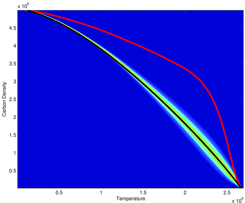
Figure 1: Joint probability density function of fuel and temperature from case (e) in Paper I. The solid red line shows the distribution from the flat laminar flame where thermal diffusion is the dominant mixing process. The solid black line shows the distribution of fuel burning isobarically with no thermal or species diffusion.

A key result from Paper I was that at high Karlovitz number ($\mathrm{Ka}\approx 230$), turbulence dominates the mixing of fuel and heat while thermal diffusion plays only a minor role. Figure 1 shows a joint probability density function (JPDF) of fuel and temperature from Paper I. The solid red line shows the distribution from the flat laminar flame where thermal diffusion is the dominant mixing process, and the solid black line shows the distribution of fuel burning isobarically with no thermal or species diffusion. The agreement with the JPDF demonstrates that the turbulent flame is burning at an effective Lewis number close to unity - the mixing is chiefly due to turbulence.

The simulations in Paper I were performed in small domains to ensure that the laminar flame was fully-resolved – the domain size was approximately twenty-five times the laminar flame width. The aim of this paper is to investigate turbulent flame speeds in larger domains, with the aim of predicting high Karlovitz flame speeds in a full star, and specifically testing predictions made in Paper I. In this paper, we will refine these predictions by giving an in-depth theoretical description of the distributed burning regime, which are then compared with one- and three-dimensional simulations.

2 THEORETICAL DESCRIPTION OF THE DISTRIBUTED BURNING REGIME

There is diversity in the literature when naming the burning regimes for large Karlovitz number. Here we use the term “distributed burning regime” (or “distributed reaction zone”) to refer collectively to all burning with large Karlovitz number ($\mathrm{Ka}\lower 0.43057pt\hbox{\hbox to0.0pt{\raise 2.58334pt\hbox{\hskip 1.29167pt{{$\scriptscriptstyle>$}}}\hss} \kern-1.72218pt{{$\scriptscriptstyle\sim$}}}10$). We also follow Woosley et al. (2009) in further subdividing this region based upon the turbulent Damköhler number, $\mathrm{Da}_{T}$, to be defined below. Specifically, $\mathrm{Da}_{T}<1$ will be referred to as the “well-stirred reactor” (see Peters (1986) or Woosley et al. (2009)) and $\mathrm{Da}_{T}>1$ as the “stirred-flame regime” (see Kerstein (2001) or Woosley et al. (2009)).

2.1 The Well-Stirred Reactor

Damköhler (1940) identified two burning regimes, which he referred to as “small-scale” and “large-scale” turbulence, see also Peters (1999, 2000). In the large-scale turbulence regime, laminar flames are dragged around by large turbulent eddies, which is an appropriate description of the burning in a Type Ia supernovae at high density (Woosley et al., 2009). The high Karlovitz number case from Paper I is in the “small-scale” turbulence regime, where the small-scale mixing is dominated by turbulence, rather than diffusion.

In this regime, the turbulent eddies are strong enough to disrupt the internal structure of the flame. The time scale of these eddies is faster than the time scale of the flame, so the flame is mixed before it can burn. Therefore, the burning takes place on an inductive time scale, or turbulent nuclear time scale, which is much slower than the laminar nuclear time scale. Damköhler predicted (by analogy with laminar flames) that the turbulent flame speed $s_{T}$ and width $l_{T}$ should depend upon the turbulent diffusion coefficient and the nuclear burning time scale,

$$s_{T}=\sqrt{\frac{\mathcal{D}_{T}}{\tau^{T}_{\mathrm{nuc}}}},\quad\mathrm{and}\quad l_{T}=\sqrt{\mathcal{D}_{T}\tau^{T}_{\mathrm{nuc}}},$$ (2)

where $\tau^{T}_{\mathrm{nuc}}$ is the turbulent nuclear time scale ($\tau^{T}_{\mathrm{nuc}}=l_{T}/s_{T}$), and $\mathcal{D}_{T}$ is the turbulent diffusion coefficient $\mathcal{D}_{T}=\alpha\check{u}l$ (not to be confused with $\mathrm{Da}_{T}$), where $\alpha$ is an order one constant. For convenience, take $\alpha=1$, which can be thought of as absorbing the constant into the definition of the turbulent flame width, which is ambiguous.

Keeping the Karlovitz number fixed (so the energy dissipation rate of the turbulence $\varepsilon^{*}=\check{u}^{3}/l$ is constant) and assuming that $\tau^{T}_{\mathrm{nuc}}$ is constant (i.e. the limiting value has been achieved), then there is only one free parameter. This parameter can be written as a turbulent Damköhler number, defined as

$$\mathrm{Da}_{T}\equiv\frac{\tau_{T}}{\tau^{T}_{\mathrm{nuc}}}=\frac{s_{T}}{\check{u}}\frac{l}{l_{T}}.$$ (3)

It is straightforward to show that $\mathrm{Da}_{T}\propto l^{2/3}$, where the constant of proportionality is $({\varepsilon^{*}}^{1/3}\tau^{T}_{\mathrm{nuc}})^{-1}$. Therefore, the free parameter can be thought of in terms of the integral length scale. Both $s_{T}$ and $l_{T}$ are proportional to $\mathcal{D}_{T}^{1/2}$, so writing $\mathcal{D}_{T}=\check{u}l={\varepsilon^{*}}^{1/3}l^{4/3}$, it follows immediately that both $s_{T}$ and $l_{T}$ scale with $l^{2/3}$ (or equivalently $\mathrm{Da}_{T}$).

2.2 The Stirred-Flame Regime

When the turbulence time scale $\tau_{T}$ becomes comparable to the turbulent nuclear time scale $\tau^{T}_{\mathrm{nuc}}$, i.e. $\mathrm{Da}_{T}\approx 1$, the turbulence on the integral length scale can no longer mix the flame before it burns. Therefore, the flame can not be broadened any further and a limiting behavior is reached. Specifically, for $\mathrm{Da}_{T}\lower 0.43057pt\hbox{\hbox to0.0pt{\raise 2.58334pt\hbox{\hskip 1.29167pt{{$\scriptscriptstyle>$}}}\hss} \kern-1.72218pt{{$\scriptscriptstyle\sim$}}}1$, the flame burns like a unity Lewis number flame (on the scale of the flame width) with local flame speed $s_{\lambda}$ and width $l_{\lambda}$. We refer to this kind of burning as a $\lambda$-flame.

Defining a turbulent Karlovitz number as

$$\mathrm{Ka}_{T}=\sqrt{\frac{\check{u}^{3}}{s_{T}^{3}}\frac{l_{T}}{l}},$$ (4)

it can be shown that $\mathrm{Da}_{T}^{2}\mathrm{Ka}_{T}^{2}=\alpha\equiv 1$. Therefore, when the scaling relations break down at $\mathrm{Da}_{T}\approx 1$, it follows immediately that the turbulent flame speed is equal to the turbulent intensity and the turbulent flame width is equal to the integral length scale.

It is the limit $\mathrm{Da}_{T}\approx 1$ that divides the distributed regime into the well-stirred reactor regime and the stirred-flame regime. In particular, note that it is the turbulent Damköhler number that is the divide, and that $\mathrm{Da}_{T}=\sigma\mathrm{Da}_{L}$, where $\sigma=\tau_{\rm nuc}^{L}/\tau_{\rm nuc}^{T}$ is the ratio of the nuclear time scales. Therefore, a $\lambda$-flame can only exist in the stirred-flame regime, i.e. $\mathrm{Da}_{T}>1$ and $\mathrm{Ka}\lower 0.43057pt\hbox{\hbox to0.0pt{\raise 2.58334pt\hbox{\hskip 1.29167pt{{$\scriptscriptstyle>$}}}\hss} \kern-1.72218pt{{$\scriptscriptstyle\sim$}}}10$.

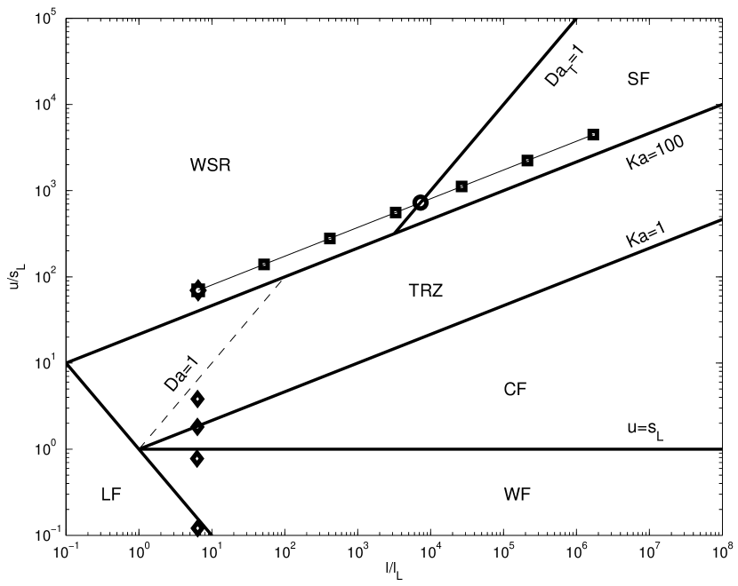
Figure 2: Regime diagram based on Peters (1999, 2000). Here we emphasize the separation of the distributed burning regime into the well-stirred reactor and stirred-flame regimes by the turbulence Damköhler number $\mathrm{Da}_{T}=1$. (LF - Laminar Flames, WF - Wrinkled Flames, CF - Corrugated Flames, TRZ - Thin Reaction Zone, WSR - Well-Stirred Reactor, SF - Stirred Flame). Together the WSR and SF regimes make up the distributed burning regime. The diamonds denote the simulations from Paper I, and the squares denote the simulations from the present paper. The circle denotes the intersect of the $\mathrm{Ka}=230$ line with $\mathrm{Da}_{T}=1$, which denotes the $\lambda$-point, where the turbulent intensity and integral length scale are equal to the turbulent flame speed ($s_{\lambda}$) and width ($l_{\lambda}$), respectively.

Figure 2 shows a regime diagram, based on Peters (1999, 2000), where we emphasize the divide in the distributed burning regime. The diamonds denote the simulations from Paper I, and the squares denote the simulations from the present paper (to be defined below). The circle denotes the intersection of the $\mathrm{Ka}=230$ line with $\mathrm{Da}_{T}=1$, which denotes the $\lambda$-point, where the turbulent intensity and integral length scale are equal to the turbulent flame speed ($s_{\lambda}$) and width ($l_{\lambda}$), respectively.

We emphasize that the $\lambda$-flame speed and width are local measures, i.e. the flame burns at $s_{\lambda}$ on a scale of $l_{\lambda}$. These quantities will also vary due to turbulent intermittency. The $\lambda$-flame will respond to the local turbulence, specifically $\varepsilon$ on the scale of $l_{\lambda}$. Note that due to this response, the turbulent Gibson scale $l_{G}^{T}=s_{\lambda}^{3}/(\check{u}^{3}/l)$ is equal to the $\lambda$-flame width, $l_{G}^{T}=l_{\lambda}$, and the Karlovitz number based on the $\lambda$-flame is always one, i.e. $\mathrm{Ka}_{\lambda}^{2}\equiv(\check{u}^{3}l_{\lambda})/(s_{\lambda}^{3}l)\equiv 1$.

The overall turbulent flame speed will be greater than $s_{\lambda}$ due to enhanced flame surface area, and will resemble Damköhler’s large-scale turbulence regime, due to the presence of multiple $\lambda$-flames across an integral length scale. Following Peters (1999), for example, the following simple expression, based on an enhanced flame surface area, can be used to illustrate the scaling behavior in this regime,

$$\frac{s_{T}}{s_{\lambda}}=1+\frac{\check{u}}{s_{\lambda}}.$$ (5)

Specifically, in the limit of high Damköhler number, the turbulent burning speed tends to the turbulent intensity, i.e. $s_{T}\rightarrow\check{u}$ as $\mathrm{Da}_{T}\rightarrow\infty$.

In the next section, we present calculations to investigate the turbulent flame speed as a function of Damköhler number for a high Karlovitz number flame. Specifically, we are looking for a relation of the form

$$\frac{s_{T}}{\check{u}}=\varphi\left(\mathrm{Da}_{T}\right),$$ (6)

for some dimensionless function $\varphi$. Three burning regimes are to be expected. First, for $\mathrm{Da}_{T}\lower 0.43057pt\hbox{\hbox to0.0pt{\raise 2.58334pt\hbox{\hskip 1.29167pt{{$\scriptscriptstyle<$}}}\hss} \kern-1.72218pt{{$\scriptscriptstyle\sim$}}}1$, the turbulent flame speed and width are predicted to scale with

$$\frac{s_{T}}{\check{u}}=\mathrm{Da}_{T}^{1/2},\quad\mathrm{and}\quad\frac{l_{T}}{l}=\mathrm{Da}_{T}^{-1/2}.$$ (7)

Second, for $\mathrm{Da}_{T}\approx 1$, the flame is predicted to reach a limiting behavior with speed $s_{\lambda}$ and width $l_{\lambda}$ (on the scale of $l_{\lambda}$). Finally, for $\mathrm{Da}_{T}\gg 1$, the flame is predicted to burn as a $\lambda$-flame, where the overall flame speed is expected to be a few times the turbulent intensity, tending towards it as $\mathrm{Da}_{T}$ tends to infinity.

2.3 The Turbulent Nuclear Time Scale

Previous work has implicitly assumed that the nuclear time scale remains unaffected by the turbulence, again see Peters (1999) or Peters (2000). This was the case in Röpke & Hillebrandt (2005), where the relation

$$\frac{s_{T}}{s_{L}}\sim\left(\frac{\mathcal{D}_{T}}{\mathcal{D}_{L}}\right)^{1/2}\sim\left(\frac{\check{u}l}{s_{L}l_{L}}\right)^{1/2},$$ (8)

was used to derive a turbulent flame speed for a level-set method. However, as discussed in Paper I, due to the different distributions of carbon and temperature, the nuclear time scale is around an order of magnitude longer in the turbulent case. Allowing for different nuclear time scales, equation (8) becomes

$$\frac{s_{T}}{s_{L}}=\left(\frac{\check{u}l}{s_{L}l_{L}}\right)^{1/2}\left(\frac{\tau_{\rm nuc}^{L}}{\tau_{\rm nuc}^{T}}\right)^{1/2}.$$ (9)

In Paper I, the turbulent nuclear time scale was estimated using $l_{T}/s_{T}$, based on an estimate of the turbulent flame width. It was shown that this reduces the estimate for the turbulent flame speed in equation 9 by a factor of approximately $\sigma^{1/2}\approx 0.3$. A more refined approach for estimating $\tau_{\rm nuc}^{T}$ is given below.

A corollary to the relation $\mathrm{Da}_{T}^{2}\mathrm{Ka}_{T}^{2}=1$, is that the turbulent nuclear time scale can be derived from a single measurement in the well-stirred reactor regime, specifically, the turbulent flame speed and properties of the turbulence alone. In particular, if we consider a reference case that is easily computed (e.g. case (e) from Paper I), where the turbulent intensity is $\check{u}_{0}$ and integral length scale $l_{0}$, then only the turbulent flame speed $s_{T}^{0}$ needs to be measured. Assuming that the limiting nuclear time scale has been achieved, then the relation $\mathrm{Da}_{T}^{2}\mathrm{Ka}_{T}^{2}=1$ means that the turbulent flame width is $l_{T}^{0}=\check{u}_{0}l_{0}/s_{T}^{0}$, and the turbulent nuclear time scale is $\tau_{\mathrm{nuc}}^{T}=l_{T}^{0}/s_{T}^{0}=\check{u}_{0}l_{0}/{s_{T}^{0}}^{2}$. For case (e) in Paper I, this gives $l_{T}\approx 190$cm, $\tau_{\rm nuc}^{T}\approx 0.0098$s, and $\sigma\approx 0.067$ (which gives $\sigma^{1/2}\approx 0.26$).

3 SIMULATION DESCRIPTION

3.1 Three-Dimensional Simulations

As in Paper I, we use a low Mach number hydrodynamics code, adapted to the study of thermonuclear flames, as described in Bell et al. (2004). The advantage of this method is that sound waves are filtered out analytically, so the time step is set by the the bulk fluid velocity and not the sound speed. This is an enormous efficiency gain for low speed flames. The input physics used in the present simulations is largely unchanged, with the exception of the addition of Coulomb screening, taken from the Kepler code (Weaver et al., 1978), to the ¹²C(¹²C,$\gamma$)²⁴Mg reaction rate. This yields a small enhancement to the flame speed, and is included for completeness. The conductivities are those reported in Timmes (2000), and the equation of state is the Helmholtz free-energy based general stellar EOS described in Timmes & Swesty (2000). We note that we do not utilize the Coulomb corrections to the electron gas in the general EOS, as these are expected to be minor at the conditions considered.

The basic discretization combines a symmetric operator-split treatment of chemistry and transport with a density-weighted approximate projection method. The projection method incorporates the equation of state by imposing a constraint on the velocity divergence. The resulting integration of the advective terms proceeds on the time scale of the relatively slow advective transport. Faster diffusion and chemistry processes are treated time-implicitly. This integration scheme is embedded in a parallel adaptive mesh refinement algorithm framework based on a hierarchical system of rectangular grid patches. The complete integration algorithm is second-order accurate in space and time, and discretely conserves species mass and enthalpy. The details of the adaptive incompressible flow solver can be found in Almgren et al. (1998), the reacting flow solver in Day & Bell (2000), extension to generalized equation of state in Bell et al. (2004), and an application to the Rayleigh-Taylor instability in type Ia SNe in Zingale et al. (2005).

The non-oscillatory finite-volume scheme employed here permits the use of implicit large eddy simulation (iles). This technique captures the inviscid cascade of kinetic energy through the inertial range, while the numerical error acts in a way that emulates the dissipative physical effects on the dynamics at the grid scale, without the expense of resolving the entire dissipation subrange. An overview of the technique can be found in Grinstein et al. (2007). Aspden et al. (2008b) presented a detailed study of the technique using the present numerical scheme, including a characterization that allowed for an effective viscosity to be derived. Thermal diffusion plays a significant role in the flame dynamics, and so is explicitly included in the model, whereas species diffusion is significantly smaller, and so is not explicitly included.

The turbulent velocity field was maintained using the forcing term used in Paper I and Aspden et al. (2008b). Specifically, a forcing term was included in the momentum equations consisting of a superposition of long wavelength Fourier modes with random amplitudes and phases. The forcing term is scaled by density so that the forcing is somewhat reduced in the ash. This approach provides a way to embed the flame in a zero-mean turbulent background, mimicking the much larger inertial range that these flames would experience in a type Ia supernova, without the need to resolve the large-scale convective motions that drive the turbulent energy cascade. The effects of resolution were examined in detail in Aspden et al. (2008b), where it was demonstrated that the effective Kolmogorov length scale is approximately $0.28\Delta x$, and the integral length scale is approximately a tenth of the domain width. This is particularly relevant to the present study, because turbulence is the dominant mixing process. This means that the iles approach can be used to capture the effects of turbulent mixing, which occurs on length scales much larger than the actual Kolmogorov length scale in the star.

Figure 3 shows the simulation setup. The simulations were initialized with carbon fuel in the lower part of the domain and magnesium ash in the upper, resulting in a downward propagating flame. A high-aspect ratio domain was used to allow the flame sufficient space to propagate. Periodic boundary conditions were prescribed laterally, along with a free-slip base, and outflow at the upper boundary.

3.2 One-Dimensional Simulations Using the Linear Eddy Model

Simulations were also run using the Linear Eddy Model (LEM) of Kerstein (1991). This approach simulates the evolution of scalar properties in a one-dimensional domain, which can be interpreted as a line of sight through a three-dimensional turbulent flow. Diffusive transport and chemical reactions are coupled in a model that represents the effects of real three-dimensional eddies through a so-called “triplet map”. The advantage of LEM is that much finer resolution and larger length scales can be explored inexpensively. This is particularly important for the present problem, where the range of length scales is very large and the degree of turbulence very high. LEM has been successfully applied to a large range of phenomena, especially turbulent terrestrial combustion. Its disadvantage is that when applied to a novel environment like a supernova, there are two overall normalization factors that must be adjusted, the effective turbulent dissipation rate and the integral scale. By using LEM for the present problem, we hope to satisfy two goals - first to show that very similar answers are obtained using quite different techniques and second, to calibrate the uncertain constants in LEM for the supernova problem.

LEM has previously been compared with the same three-dimensional code in Woosley et al. (2009). When the nuclear physics and fuel temperature were adjusted to be the same, it was found that best agreement occurred for an LEM constant $C$ = 11 and an integral scale in LEM that was three times that in the numerical simulation. Those same values are used here except that $C$ has been assumed to be 10. As expected, this prescription gives excellent agreement in the well-stirred reactor regime where it was calibrated, but, as we shall see underestimates the flame speed by as much as a factor of two in the stirred-flame regime. Thus a normalization that depends on $\mathrm{Da}_{T}$ is appropriate, and $C$ = 3 to 5 for $\mathrm{Da}_{T}>1$.

4 RESULTS

4.1 Three-Dimensional Results

The high Karlovitz case from Paper I was used as the starting point for the present study, and is referred to here as case (a). Because turbulent diffusion dominates the mixing of fuel and temperature, the resolution requirements are significantly relaxed – thermal diffusion has to be resolved to capture the laminar flame correctly, but the turbulent diffusion coefficient is much larger, and so fewer cells are required to resolve it. In fact, keeping $\varepsilon^{*}$ constant means that the diffusion coefficient scales with $\mathcal{D}_{T}\sim l^{4/3}$, and a mixing length can be defined analogous to the Kolmogorov length scale $\eta_{\mathcal{D}}=(\mathcal{D}_{T}^{3}/\varepsilon^{*})^{1/4}$, which scales as $\eta_{\mathcal{D}}\sim l$. Thus, the smallest scales that need to be resolved become larger as the domain size grows.

The approach taken to achieve larger Damköhler numbers (i.e. larger length scales) was to start with case (a), which has a domain width of $1.5\times 10^{2}$cm, and run the same case at an eighth of the resolution, i.e. with a low-resolution cell width of $\Delta x_{LR}=\Delta x_{HR}/8$. The turbulent flame speed was used as the primary diagnostic. Agreement in the turbulent flame speed provides confidence in capturing the effects of turbulent mixing (relying on the iles approach) with the new cell width; it is the turbulent flame speed that is of primary interest. A higher Damköhler number was then achieved by running in a domain eight times larger with the new cell width, i.e. with a domain size of $1.2\times 10^{3}$cm. The turbulent intensity was adjusted accordingly to keep $\varepsilon^{*}=\check{u}^{3}/l$ constant (i.e. an eight-fold increase in length scale corresponds to a two-fold increase in velocity). The whole process was then repeated several times to reach a domain size of $6.14\times 10^{5}$cm, and span a range of Damköhler numbers from the base case of $\mathrm{Da}_{T}\approx 0.0064$ to $\mathrm{Da}_{T}\approx 1.68$, corresponding to cases (a) through (e).

For larger length scales, the above argument no longer applies because the diffusion coefficient responsible for mixing fuel and temperature is approximately $s_{\lambda}l_{\lambda}$ and does not scale with $\check{u}l$ for $\mathrm{Da}_{T}\lower 0.43057pt\hbox{\hbox to0.0pt{\raise 2.58334pt\hbox{\hskip 1.29167pt{{$\scriptscriptstyle>$}}}\hss} \kern-1.72218pt{{$\scriptscriptstyle\sim$}}}1$; even case (e) is questionably resolved. However, we have included simulations (f) and (g) at Damköhler numbers 6.6 and 26, respectively, as an indication of what we can expect for $\mathrm{Da}_{T}\lower 0.43057pt\hbox{\hbox to0.0pt{\raise 2.58334pt\hbox{\hskip 1.29167pt{{$\scriptscriptstyle>$}}}\hss} \kern-1.72218pt{{$\scriptscriptstyle\sim$}}}1$. The simulation properties are summarized in table 1.

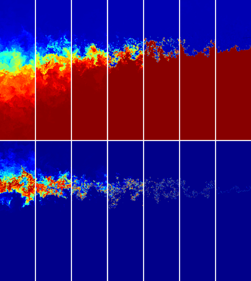
Figure 4: Two-dimensional slices showing density (top) and fuel consumption rate (bottom) for all cases (a)-(g) (left-to-right). All of the figures have been normalized by the same values. It is important to note the domain increases by a factor of 8 each time. In particular, the domain size in the final case is over two hundred and fifty thousand times larger than the first case; despite the burning rate looking reduced, it is actually greatly increased.

Figure 4 shows slices of density (top) and fuel consumption rate (bottom) for the seven cases (a)-(g) left-to-right. Note that the domain size increases by a factor of 8 each time. All of the figures have been normalized by the same values. Case (a) presents an extremely broad mixing region (much broader than the integral length scale), and the burning can be seen to occur at the high temperature (low density) end of the mixing zone. As the Damköhler number is increased, the relative width of the flame brush decreases as expected. Although the width of the flame brush appears to decrease, it actually increases, just more slowly than the domain size. For $\mathrm{Da}_{T}\lower 0.43057pt\hbox{\hbox to0.0pt{\raise 2.58334pt\hbox{\hskip 1.29167pt{{$\scriptscriptstyle>$}}}\hss} \kern-1.72218pt{{$\scriptscriptstyle\sim$}}}1$, there appears to be a sharp interface between the fuel and products. This is because of the underresolved nature of the flames - the actual flame will be a broad mixing zone, but is not fully-captured here.

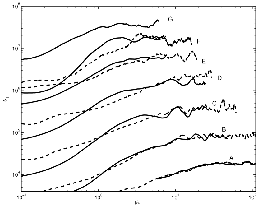
Figure 5: Turbulent flame speeds $s_{T}$ as a function of time (normalized by turbulent time scale $\tau_{T}$. The solid lines denote the simulations at the full resolution ($256^{2}$ cells in cross-section), and the dashed lines denote the simulations at the low resolution ($32^{2}$ cells in cross-section).

Figure 5 shows the turbulent flame speed evolution for the seven cases. The flame speed is evaluated by finding the rate of change of the total fuel mass in the domain divided by the product of the cross-sectional area of the domain and the fuel density,

$$s_{T}=\frac{1}{A(\rho X_{C})_{0}}\frac{\mbox{d}}{\mbox{d}t}\int_{V}{\rho X_{C}\,\mbox{d}V}.$$ (10)

The time scale has been normalized by the eddy turnover time $\tau_{T}=l/\check{u}$. The solid lines denote the simulations at the full resolution ($256^{2}$ cells in cross-section), and the dashed lines denote the simulations at the low resolution ($32^{2}$ cells in cross-section). In most cases the low resolution simulations are in good agreement with the high resolution simulations (the only real outlier is case (d) where the low resolution simulation over-predicts the flame speed by 48%). Table 2 shows the mean flame speeds at both resolutions in each case.

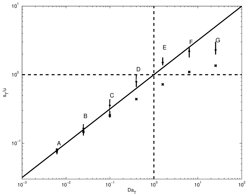
Figure 6: Turbulent flame speeds normalized by turbulent intensity $s_{T}/\check{u}$ as a function of turbulent Damköhler number $\mathrm{Da}_{T}$. The solid black line denotes the expected scaling behavior for $\mathrm{Da}_{T}\lower 0.43057pt\hbox{\hbox to0.0pt{\raise 2.58334pt\hbox{\hskip 1.29167pt{{$\scriptscriptstyle<$}}}\hss} \kern-1.72218pt{{$\scriptscriptstyle\sim$}}}1$, bounded by the dashed lines. The flame speeds appear to be in good agreement with the predicted scaling, and despite the lack of resolution, appear to roll over when $\mathrm{Da}_{T}\lower 0.43057pt\hbox{\hbox to0.0pt{\raise 2.58334pt\hbox{\hskip 1.29167pt{{$\scriptscriptstyle>$}}}\hss} \kern-1.72218pt{{$\scriptscriptstyle\sim$}}}1$. The crosses denote the mean speeds from the LEM calculations.

Figure 6 shows the turbulent burning speeds normalized by the turbulent intensity as a function of Damköhler number. Case (a) is the low Damköhler number on the left, increasing to the right to case (g). The marker denotes the mean in each case, and the vertical line denotes the range of values obtained during the averaging period (note that it is not the standard deviation). The solid line is the expected scaling relation from equation 7. The dashed lines denote $\mathrm{Da}_{T}=1$ and $s_{T}=\check{u}$, where the scaling relation is predicted to break down. Cases (a)-(e) are in very good agreement with the predicted scaling. We note that for cases (d) and (e), the flame speed measured is enhanced by the area of the flame that is burning, which can be increased by turbulence here because the flame brush is now smaller than the domain width; this explains the higher speeds obtained. The flames in these cases are too convoluted to extract a flame area to normalize by. Despite being significantly underresolved, cases (f) and (g) appear to show the expected break-down of the Damköhler scaling; for $\mathrm{Da}_{T}\lower 0.43057pt\hbox{\hbox to0.0pt{\raise 2.58334pt\hbox{\hskip 1.29167pt{{$\scriptscriptstyle>$}}}\hss} \kern-1.72218pt{{$\scriptscriptstyle\sim$}}}1$, the turbulence cannot enhance the flame speed according to equation (7), and the normalized flame speed ceases to grow.

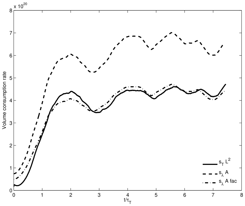
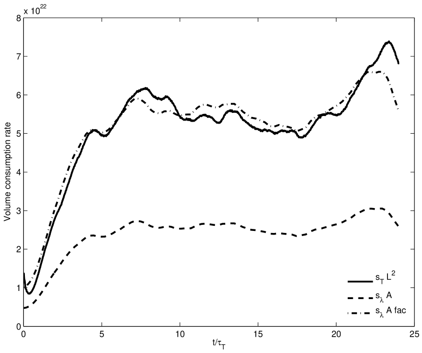
Figure 7: Volumetric rate of fuel consumption. The solid line is the measured rate $As_{T}$, where $A$ is the cross-sectional area, the dotted line is the product of the limiting flame speed $s_{\lambda}$ with the measured flame surface area, and the dash-dotted line is the latter adjusted by a factor of $0.67$ for case (f) and $2.16$ for case (g). There is a definite correlation between the flame surface area and the fuel consumption, but the estimate $s_{\lambda}$ appears to be an over-prediction for case (f) and an under-prediction for case (g). We speculate that this is due to the underresolved nature of these cases and that $s_{\lambda}$ is still a reasonable estimate for a turbulent flame model.

Figure 7 compares the volumetric rate of burning for cases (f) and (g). Because these two cases are much less convoluted than cases (a)-(e) it was possible to extract an isosurface based on a temperature of $10^{9}$K. The solid line denotes the measured turbulent flame speed multiplied by the cross-sectional area of the domain, the dashed line denotes the measured flame surface area times the predicted burning speed $s_{\lambda}$. It appears that the flame speed is over-predicted in case (f) and under-predicted in case (g); the dash-dotted line denotes this speed multiplied by a factor of $0.67$ for case (f) and $2.16$ for case (g). We speculate that the disagreement is due to the underresolved nature of these cases, but maintain that $s_{\lambda}$ is still a reasonable estimate for a turbulent flame model.

4.2 One-Dimensional Results

LEM was used to simulate the same conditions as in Table 1 except that in each case the integral scale was multiplied by three and finer resolution was employed (Table 3). Roughly 40,000 time points were sampled for each case. The average flame speeds are plotted in Figure 6. For $\mathrm{Da}_{T}\lower 0.43057pt\hbox{\hbox to0.0pt{\raise 2.58334pt\hbox{\hskip 1.29167pt{{$\scriptscriptstyle<$}}}\hss} \kern-1.72218pt{{$\scriptscriptstyle\sim$}}}1$, the agreement with the three-dimensional simulations is excellent. Both show the same scaling relation as well as agreeing on the actual value of the speed. However, at large values of $\mathrm{Da}_{T}$, the LEM results are almost a factor of two smaller. There could be several reasons for this. First, there are fundamental differences in the two approaches. LEM does not capture all of the multi-dimensional effects and has not been calibrated for this regime. Second, the resolution of the three-dimensional study is low and not all burning structures are well resolved. Studies with LEM suggest a mild dependence of $s_{T}$ on the resolution with slower speeds at higher resolution.

4.3 Variability of the Turbulent Flame Speed

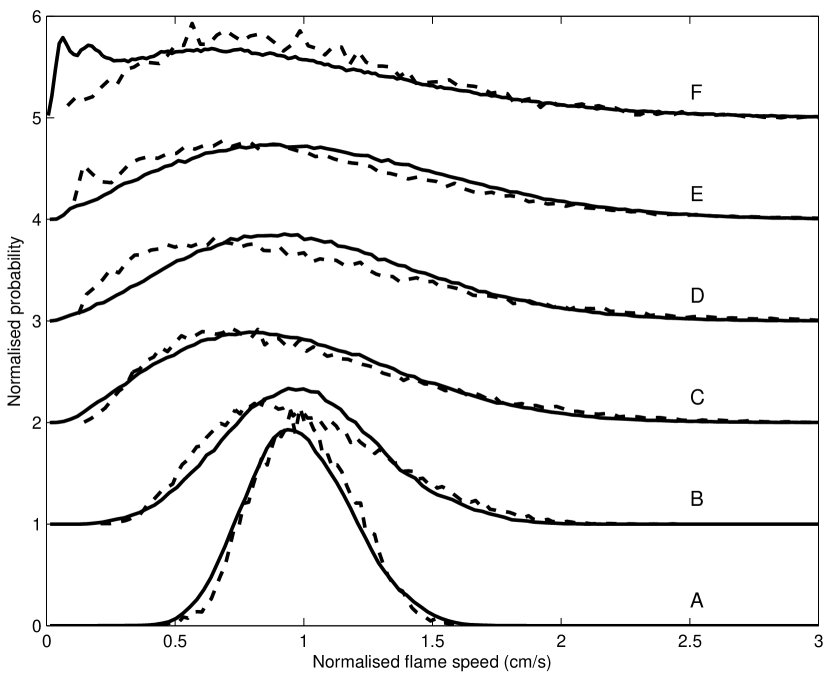
Figure 8: Probability density functions of normalized local burning rate for both the 3D (solid) and LEM (dashed) calculations. Each case has been shifted along the $y$-axis for clarity.

Figure 8 compares the probability density functions (PDFs) of the normalized local burning rate in the three-dimensional and LEM calculations. To compare the three-dimensional results as closely as possible with LEM, the PDFs were evaluated by integrating the fuel consumption along line-outs, i.e. over individual columns of data as a function of height. Each PDF was then normalized by the mean burning speed. The PDFs have been shifted along the $y$-axis for clarity. In case (a), the PDF has a narrow Gaussian distribution centered around the mean flame speed. As the Damköhler number increases, the PDF becomes broader, i.e. a greater range of burning rates is observed locally.

Both studies show a strong dependence of the spread of the PDF on Damköhler number. In the well-stirred reactor ($\mathrm{Da}_{T}<1$), the integral scale is less than the flame width. Many eddies turn over on the largest scale as burning moves through a region. The relation between temperature, carbon mass fraction, and location is smooth and the burning time well defined. There is only one flame structure. Consequently the speed does not vary greatly from the average.

In the stirred flame, however, there are multiple regions of burning. Sometimes the burning is very fast, especially when a large single eddy envelops a new region of fuel. At other times it, almost goes out. The PDF thus shows a large spread in speed. Occasionally, the overall burning proceeds at a rate that is 2.5 to 3 times the average. Since the average itself if roughly twice $\check{u}$, this implies an overall burning rate up to six times $\check{u}$.

5 CONCLUSIONS

New one- and three-dimensional simulations have been presented to clarify and quantify the nature of carbon burning in a Type Ia supernova in the distributed burning regime. The characteristics of distributed burning depend upon the Damköhler number, and a range of $\mathrm{Da}_{T}$ from 0.006 to 26 has been explored. For $\mathrm{Da}\lower 0.43057pt\hbox{\hbox to0.0pt{\raise 2.58334pt\hbox{\hskip 1.29167pt{{$\scriptscriptstyle<$}}}\hss} \kern-1.72218pt{{$\scriptscriptstyle\sim$}}}1$, the expected scaling relations were demonstrated,

$$\frac{s_{T}}{\check{u}}=\mathrm{Da}_{T}^{1/2},\quad\mathrm{and}\quad\frac{l_{T}}{l}=\mathrm{Da}_{T}^{-1/2}.$$ (11)

For $\mathrm{Da}_{T}\lower 0.43057pt\hbox{\hbox to0.0pt{\raise 2.58334pt\hbox{\hskip 1.29167pt{{$\scriptscriptstyle>$}}}\hss} \kern-1.72218pt{{$\scriptscriptstyle\sim$}}}1$, these relations break down and the turbulent flame reaches a maximum local flame speed $s_{\lambda}$ and width $l_{\lambda}$, measured on the scale of $l_{\lambda}$. This $\lambda$-flame interacts with turbulent eddies with length scales between $l_{\lambda}$ and the integral length scale $l$, which enhances the flame surface area. The average turbulent flame properties are constrained by the large scales (see also Woosley et al., 2009). This leads to an average overall turbulent flame speed, which to factor-of-two accuracy is given by the turbulent intensity, $\check{u}$. For the range of $\mathrm{Da}\lower 0.43057pt\hbox{\hbox to0.0pt{\raise 2.58334pt\hbox{\hskip 1.29167pt{{$\scriptscriptstyle>$}}}\hss} \kern-1.72218pt{{$\scriptscriptstyle\sim$}}}1$ studied here, a good approximation is $s_{T}=2\check{u}$.

5.1 Consequences for Large-Scale Simulations

Large-scale simulations (i.e. of a full-star) will require a turbulent flame model. One of the consequences of the results presented here is that the $\lambda$-flame is ideally suited to the level-set approach, as it burns locally with speed $s_{\lambda}$. This means that a turbulent flame speed can be evaluated in the following manner. Assume that the turbulence is sufficiently large and intense, i.e. in the stirred-flame regime ($\mathrm{Da}_{T}>1$ and $\mathrm{Ka}\lower 0.43057pt\hbox{\hbox to0.0pt{\raise 2.58334pt\hbox{\hskip 1.29167pt{{$\scriptscriptstyle>$}}}\hss} \kern-1.72218pt{{$\scriptscriptstyle\sim$}}}10$). Then the turbulence can be characterized by the energy dissipation rate $\varepsilon^{*}=\check{u}^{3}/l$, and the burning depends on the turbulent nuclear burning time scale $\tau_{\mathrm{nuc}}^{T}$. The nuclear burning time scale is equal to $l_{\lambda}/s_{\lambda}$ and the turbulent intensity at the length scale of the $\lambda$-flame is $s_{\lambda}$ and so $\varepsilon^{*}=s_{\lambda}^{3}/l_{\lambda}$. Solving for $s_{\lambda}$ and $l_{\lambda}$ gives

$$s_{\lambda}=\sqrt{\varepsilon^{*}\tau_{\mathrm{nuc}}^{T}},\quad\mathrm{and}\quad l_{\lambda}=\sqrt{\varepsilon^{*}{\tau_{\mathrm{nuc}}^{T}}^{3}}.$$ (12)

Note these expressions do not require a fixed Karlovitz number (it’s incorporated by $\varepsilon^{*}$), and the the length scale is the same as predicted in Paper I. To implement a level-set approach for a $\lambda$-flame, $\tau_{\mathrm{nuc}}^{T}$ should be evaluated as a function of fuel density and temperature (using the approach outlined in section 2.1 or Woosley et al. (2009)) and coupled with the (local) energy dissipation rate to evaluate the $\lambda$-flame speed according to equation (12). If the resolution requirements of Paper I were applied to the $\lambda$-flame recovered in the present paper (i.e. $l_{\lambda}\approx 4\Delta x$ with $256^{2}$ cells in cross-section), an integral length scale could be achieved that is of order thousands of times larger than the original study.

5.2 Consequences for Detonation

The instantaneous flame speed for $\mathrm{Da}_{T}\lower 0.43057pt\hbox{\hbox to0.0pt{\raise 2.58334pt\hbox{\hskip 1.29167pt{{$\scriptscriptstyle>$}}}\hss} \kern-1.72218pt{{$\scriptscriptstyle\sim$}}}1$ is irregular, with frequent excursions up to 2.5 times the average, which is approximately twice the turbulent intensity for the simulations presented here. These variations could be crucial if a transition to detonation is to occur. Detonation will not happen in the laminar regime, i.e. at high density, because each flamelet burns at a steady rate and has a thickness that is far below the critical mass for detonation. It is also unlikely to happen in the well-stirred reactor regime, because the burning is steady and slower than the turbulence on the integral scale, which in turn is subsonic. The burning time scale is very long in the well-stirred regime, making it very difficult to burn, for example, a 10 km region on a sound crossing time.

Thus if detonation is to occur spontaneously, it is likely to happen in the stirred-flame regime. Even there though, $\mathrm{Da}_{T}$ should not be too large, or the mixed regions will not burn supersonically (recall $s_{T}\rightarrow\check{u}$ for large $\mathrm{Da}_{T}$). The best conditions therefore occur where there are multiple $\lambda$-flames across an integral length scale, i.e. for small $\mathrm{Da}_{T}\lower 0.43057pt\hbox{\hbox to0.0pt{\raise 2.58334pt\hbox{\hskip 1.29167pt{{$\scriptscriptstyle>$}}}\hss} \kern-1.72218pt{{$\scriptscriptstyle\sim$}}}1$ (Woosley, 2007; Woosley et al., 2009). The calibration of LEM determined by comparison with the three-dimensional studies suggest a normalization constant of $C=5$ is most appropriate for $\mathrm{Da}>1$ and this is the value used by Woosley et al. (2009). This strengthens their conclusion that a detonation is possible if $\check{u}$ exceeds about one-fifth sonic.

Figure 3: Diagram of the simulation setup (shown in two-dimensions for clarity). The domain is initialized with a turbulent flow and a flame is introduced into the domain, oriented to that the flame propagates toward the lower boundary. The turbulence is maintained by adding a forcing term to the momentum equations. The top and bottom boundaries are outflow and solid wall boundaries, respectively. The side boundaries are periodic.

Case	(a)	(b)	(c)	(d)	(e)	(f)	(g)
Domain width, $L$ (cm)	$1.5\times 10^{2}$	$1.2\times 10^{3}$	$9.6\times 10^{3}$	$7.68\times 10^{4}$	$6.14\times 10^{5}$	$4.92\times 10^{6}$	$3.93\times 10^{7}$
Domain height, $H$ (cm)	$1.2\times 10^{3}$	$4.8\times 10^{3}$	$3.84\times 10^{4}$	$3.07\times 10^{5}$	$2.46\times 10^{6}$	$1.97\times 10^{7}$	$1.57\times 10^{8}$
Integral length scale, $l$ (cm)	$1.5\times 10^{1}$	$1.2\times 10^{2}$	$9.6\times 10^{2}$	$7.68\times 10^{3}$	$6.14\times 10^{4}$	$4.92\times 10^{5}$	$3.93\times 10^{6}$
Turbulent intensity, $\check{u}$ (cm/s)	$2.47\times 10^{5}$	$4.93\times 10^{5}$	$9.86\times 10^{5}$	$1.97\times 10^{6}$	$3.95\times 10^{6}$	$7.89\times 10^{6}$	$1.58\times 10^{7}$
Laminar Damköhler, $\mathrm{Da}_{L}$	$9.32\times 10^{-2}$	$3.73\times 10^{-1}$	$1.49\times 10^{0}$	$5.97\times 10^{0}$	$2.39\times 10^{1}$	$9.54\times 10^{1}$	$3.82\times 10^{2}$
Turbulent Damköhler, $\mathrm{Da}_{T}$	$6.23\times 10^{-3}$	$2.49\times 10^{-2}$	$9.97\times 10^{-1}$	$3.99\times 10^{-1}$	$1.60\times 10^{0}$	$6.38\times 10^{0}$	$2.55\times 10^{1}$
High resolution ($N=256$) $\Delta x_{HR}$ (cm)	$5.86\times 10^{-1}$	$4.69\times 10^{0}$	$3.75\times 10^{1}$	$3.00\times 10^{2}$	$2.40\times 10^{3}$	$1.92\times 10^{4}$	$1.54\times 10^{5}$
Low resolution ($N=32$) $\Delta x_{LR}$ (cm)	$4.69\times 10^{0}$	$3.75\times 10^{1}$	$3.00\times 10^{2}$	$2.40\times 10^{3}$	$1.92\times 10^{4}$	$1.54\times 10^{5}$	$1.23\times 10^{6}$

Table 1: Simulation properties.

Case	(a)	(b)	(c)	(d)	(e)	(f)	(g)
High resolution (cm/s)	$1.84\times 10^{4}$	$8.10\times 10^{4}$	$3.51\times 10^{5}$	$1.56\times 10^{6}$	$5.94\times 10^{6}$	$1.66\times 10^{7}$	$3.49\times 10^{7}$
Low resolution (cm/s)	$1.86\times 10^{4}$	$8.57\times 10^{4}$	$3.91\times 10^{5}$	$2.31\times 10^{6}$	$6.5\times 10^{6}$	$1.62\times 10^{7}$	$3.16\times 10^{7}$
Percentage error	1.1	5.8	11.4	48.1	9.4	-2.4	-9.5

Table 2: Measured turbulent flame speeds.

Case	(a)	(b)	(c)	(d)	(e)	(f)	(g)
Turbulent intensity, $\check{u}$ (cm/s)	$2.47\times 10^{5}$	$4.93\times 10^{5}$	$9.86\times 10^{5}$	$1.97\times 10^{6}$	$3.95\times 10^{6}$	$7.89\times 10^{6}$	$1.58\times 10^{7}$
Integral length scale, $l$ (cm)	$4.50\times 10^{1}$	$3.60\times 10^{2}$	$2.88\times 10^{3}$	$2.30\times 10^{4}$	$1.84\times 10^{5}$	$1.48\times 10^{6}$	$1.18\times 10^{7}$
Resolution, $\Delta x$ (cm)	$4.89\times 10^{-1}$	$2.93\times 10^{0}$	$1.47\times 10^{1}$	$9.77\times 10^{1}$	$7.32\times 10^{2}$	$2.44\times 10^{3}$	$2.44\times 10^{4}$
Average speed (cm/s)	$1.96\times 10^{4}$	$7.26\times 10^{4}$	$2.50\times 10^{5}$	$8.70\times 10^{5}$	$2.85\times 10^{6}$	$8.36\times 10^{6}$	$2.14\times 10^{7}$

Table 3: Characteristics of LEM studies.

References

- Almgren et al. (1998) Almgren, A. S., Bell, J. B., Colella, P., Howell, L. H., & Welcome, M. 1998, J. Comput. Phys., 142, 1
- Aspden et al. (2008a) Aspden, A. J., Bell, J. B., Day, M. S., Woosley, S. E., & Zingale, M. 2008a, ApJ, 689, 1173
- Aspden et al. (2008b) Aspden, A. J., Nikiforakis, N., Dalziel, S. B., & Bell, J. B. 2008b, Communications in Applied Mathematics and Computational Science, 3, 101
- Bell et al. (2004) Bell, J. B., Day, M. S., Rendleman, C. A., Woosley, S. E., & Zingale, M. A. 2004, Journal of Computational Physics, 195, 677
- Damköhler (1940) Damköhler, G. 1940, Z. Elektrochem, 46, 601
- Day & Bell (2000) Day, M. S., & Bell, J. B. 2000, Combust. Theory Modelling, 4, 535
- Grinstein et al. (2007) Grinstein, F. F., Margolin, L. G., & Rider, W. J. 2007, Implicit Large Eddy Simulation (Cambridge University Press)
- Kerstein (1991) Kerstein, A. R. 1991, Journal of Fluid Mechanics, 231, 361
- Kerstein (2001) —. 2001, Phys. Rev. E, 64, 066306
- Peters (1986) Peters, N. 1986, in 21st Symposium (International) on Combustion/The Combustion Institute, 1231–1250
- Peters (1999) Peters, N. 1999, Journal of Fluid Mechanics, 384, 107
- Peters (2000) —. 2000, Turbulent Combustion (Cambridge University Press)
- Röpke & Hillebrandt (2005) Röpke, F. K., & Hillebrandt, W. 2005, A&A, 429, L29
- Timmes (2000) Timmes, F. X. 2000, ApJ, 528, 913
- Timmes & Swesty (2000) Timmes, F. X., & Swesty, F. D. 2000, ApJs, 126, 501
- Weaver et al. (1978) Weaver, T. A., Zimmerman, G. B., & Woosley, S. E. 1978, ApJ, 225, 1021
- Woosley (2007) Woosley, S. E. 2007, ApJ, 668, 1109
- Woosley et al. (2009) Woosley, S. E., Kerstein, A. R., Sankaran, V., Aspden, A. J., & Röpke, F. 2009, ApJ, 704, 255
- Zingale et al. (2005) Zingale, M., Woosley, S. E., Rendleman, C. A., Day, M. S., & Bell, J. B. 2005, ApJ, 632, 1021