Scaling and intermittency in incoherent $\alpha$–shear dynamo

Abstract

We consider mean-field dynamo models with fluctuating $\alpha$ effect, both with and without large-scale shear. The $\alpha$ effect is chosen to be Gaussian white noise with zero mean and a given covariance. In the presence of shear, we show analytically that (in infinitely large domains) the mean-squared magnetic field shows exponential growth. The growth rate of the fastest growing mode is proportional to the shear rate. This result agrees with earlier numerical results of Yousef et al. (2008) and the recent analytical treatment by Heinemann et al. (2011) who use a method different from ours. In the absence of shear, an incoherent $\alpha^{2}$ dynamo may also be possible. We further show by explicit calculation of the growth rate of third and fourth order moments of the magnetic field that the probability density function of the mean magnetic field generated by this dynamo is non-Gaussian.

1 Introduction

The dynamo mechanism that generates large-scale magnetic fields in astrophysical objects is a topic of active research. Almost all astrophysical bodies, e.g., the Galaxy, or the Sun, show presence of large-scale shear (differential rotation). It is now well established that this shear is an essential ingredient in the dynamo mechanism. This view is also supported by direct numerical simulations (DNS). In particular, DNS of convective flows have been able to generate large-scale dynamos predominantly in the presence of shear (Käpylä et al., 2008; Hughes & Proctor, 2009), while non-shearing large-scale dynamos are only possible at very high rotation rates (Käpylä et al., 2009). The other vital constituent of the large-scale dynamo mechanism is helicity of the flow which is often described by the $\alpha$ effect. Indeed most dynamos, including the early model by Parker (1955), are the result of an $\alpha$ effect combined with shear. Of these two ingredients, shear is typically constant over the time scale of generation of the dynamo. For the case of the solar dynamo, shear or differential rotation are constrained by helioseismology. By contrast, measuring the $\alpha$ effect is a non-trivial exercise. Whenever it has been obtained from DNS studies, it was found to have large fluctuations in space and time; see e.g., Brandenburg et al. (2008) for the PDF of different components of the $\alpha$ tensor and Cattaneo & Hughes (1996) for the fluctuating time series of the total electromotive force, which is however different from the $\alpha$ effect. What effect do these fluctuations have on the properties of the $\alpha$–shear dynamo? In particular, can a fluctuating $\alpha$ effect about a zero mean drive a large-scale dynamo in conjunction with shear? Recent DNS studies (Brandenburg, 2005a; Yousef et al., 2008; Brandenburg et al., 2008, hereafter referred to as BRRK) suggest that the answer to this question is yes. Yousef et al. (2008) have further provided compelling evidence that the growth rate of the large-scale magnetic energy in such dynamos scales linearly with the shear rate, and the wavenumber of the fastest growing mode scales as the square root of the shear rate. It has been proposed that such a dynamo can also emerge by an alternate mechanism (which has nothing to do with fluctuations of the $\alpha$ effect) involving the interaction between shear and mean current density. This mechanism is called the shear–current effect (Rogachevskii & Kleeorin, 2003). However recent DNS studies of BRRK as well as those of Brandenburg (2005b) have not found evidence in support of it, and analytical works (Rädler & Stepanov, 2006; Rüdiger & Kitchatinov, 2006; Sridhar & Subramanian, 2009), for small magnetic Reynolds number, have doubted its existence. Furthermore, the shear–current effect does not produce the observed scaling, namely, growth-rate scales with the shear rate squared, and the wavenumber of the fastest growing mode scales linearly with the shear rate; see Section 4.2 of BRRK.

It behooves us then to consider the interaction between fluctuating $\alpha$ effect and shear as a possible dynamo mechanism. Kraichnan (1976) was first to propose that fluctuations of kinetic helicity can give rise to negative turbulent diffusivities, thereby giving rise to a dynamo that is effective only in small scales (Moffatt, 1978). However, more relevant in the present context is the work of Vishniac & Brandenburg (1997), who have investigated (using numerical tools) an one-dimensional model and (with analytical techniques) a simple mean-field model in a one-mode truncation with shear and fluctuating $\alpha$ effect. These models they referred to as incoherent $\alpha$–$\Omega$ dynamos. By dividing the poloidal field component by the toroidal one, they turned the mean-field dynamo equations with multiplicative noise into one with additive noise of Langevin type. They drew an analogy between the behaviour of the mean magnetic field and Brownian motion in the sense that the mean field does not grow although the mean-square field grows with a growth rate that scales with shear rate to the $2/3$ power.

Over the last decade, the problem has been studied using a variety of different approaches (Sokolov, 1997; Silant’ev, 2000; Fedotov et al., 2006; Proctor, 2007; Kleeorin & Rogachevskii, 2008; Sur & Subramanian, 2009). Models with fluctuating $\alpha$ effect, which depend on both space and time, can be divided into two categories, one in which $\alpha$ is inhomogeneous (Silant’ev, 2000; Proctor, 2007; Kleeorin & Rogachevskii, 2008) and the other in which it is a constant in space. (There are other technical differences in the two approaches as well.) In this paper we shall confine ourselves to the second class of models. For the first category, using a multiscale expansion, Proctor (2007) found a quadratic dependence of growth rate on shear rate. This result is contradicted by Kleeorin & Rogachevskii (2008) who found that the mean field averaged over $\alpha$ does not show a dynamo and that the fluctuating $\alpha$ effect adds to the diagonal components of the turbulent magnetic diffusivity tensor. Heinemann et al. (2011) have recently proposed a simple analytically tractable model, in which they consider the first and second moments (calculated over the distribution of $\alpha$) of the horizontally averaged mean field. The first moment shows the absence of dynamo effect, but the second moment shows exponential growth with the same scaling behaviour observed by Yousef et al. (2008). Motivated by their study, we solve here a similar model using a technique known as Gaussian integration by parts to obtain the same results. We further show that, even in the absence of shear, it may be possible for incoherent $\alpha^{2}$ dynamos to operate. For the model of Vishniac & Brandenburg (1997) we can also calculate the higher (third and fourth) order moments of the magnetic field to demonstrate that the probability distribution function (PDF) of the mean magnetic field generated by an incoherent $\alpha$–shear dynamo is non-Gaussian.

2 Mean-field model

Our mean-field model is designed to describe the simulations of Yousef et al. (2008) and BRRK. In particular, there is a large-scale velocity given by ${\overline{\bm{U}}}=Sx{\bm{e}}_{y}$. The turbulence is generated by an isotropic external random force with zero net helicity. The mean fields are defined by averaging over two coordinate directions $x$ and $y$. By assuming shearing-periodic boundary conditions, as done in the simulations, this averaging obeys the Reynolds rules. By virtue of the divergence-less property of the mean magnetic field, v.i.z., $\partial_{j}\bar{B}_{j}=0$, and in the absence of an imposed mean field, $\bar{B}_{z}$ can be set to zero. The resultant mean-field equations then have the following form (BRRK)

$$\partial_{t}\bar{B}_{x}=-\alpha_{yx}\partial_{z}\bar{B}_{x}-\alpha_{yy}\partial_{z}\bar{B}_{y}-\eta_{yx}\partial^{2}_{z}\bar{B}_{y}+\eta_{yy}\partial^{2}_{z}\bar{B}_{x},$$ (1)

$$\partial_{t}\bar{B}_{y}=S\bar{B}_{x}+\alpha_{xx}\partial_{z}\bar{B}_{x}+\alpha_{xy}\partial_{z}\bar{B}_{y}-\eta_{xy}\partial^{2}_{z}\bar{B}_{x}+\eta_{xx}\partial^{2}_{z}\bar{B}_{y}.\;$$ (2)

Here, $\bar{B}_{x}$ and $\bar{B}_{y}$ are the $x$ and $y$ components of the mean (averaged over $x$ and $y$ coordinate directions) magnetic field, $\eta_{ij}$ are the four relevant components of the turbulent magnetic diffusivity tensor and $\alpha_{ij}$ are the four relevant components of the $\alpha$ tensor. The shear–current effect works via a non-zero $\eta_{yx}$, provided its sign is the same as that of $S$. In this paper we do not consider the possibility of the shear–current effect; hence we set $\eta_{yx}=0$. Here we have ignored the molecular diffusivity, as we are interested in the limit of very high magnetic Reynolds numbers.

The fluctuating $\alpha$ effect is modelled by choosing each component of the $\alpha$ tensor to be an independent Gaussian random number with zero mean and the following covariance (no summation over repeated indices is assumed):

$$\langle\alpha_{ij}(t)\alpha_{kl}(t^{\prime})\rangle=D_{ij}\delta_{ik}\delta_{jl}\delta(t-t^{\prime}).$$ (3)

We also assume that the $\alpha_{ij}$s are constants in space. Note that DNS studies of BRRK have shown that the coefficients of turbulent diffusivity also show fluctuations in time, but we have ignored that in this paper. To make our notation fully transparent, let us clearly distinguish between two different kinds of averaging we need to perform. The mean fields themselves are constructed by Reynolds averaging, which in our case is horizontal averaging, and is denoted by an overbar. As we are dealing with mean field models, the quantities appearing in our equations have already been Reynolds averaged. But, as the $\alpha_{ij}$ in our mean field equation are stochastic, we study the properties of our model by writing down evolution equations for different moments of the mean magnetic field averaged over the statistics of $\alpha_{ij}$. This is denoted by the symbol $\langle\cdot\rangle$. To give an example, the first moment (mean over statistics of $\alpha$) of the $x$ component of the mean magnetic field is denoted by $\langle\bar{B}_{x}\rangle$ and the second moment (mean square) is denoted by $\langle\bar{B}_{x}^{2}\rangle$.

In numerical studies, such averaging has to be performed by averaging over sufficiently many simulations with independent realisations of noise, as was done by Sur & Subramanian (2009). In controlled experimental setup such ensemble averaging is done by executing the experiment several times with idential initial conditions. In nature we expect the noise to have a finite correlation length. Averaging over different realisation of the noise can then be done by averaging over spatial domains of size larger than the correlation length of the noise. Note further that in the present case the components of $\bar{\bm{B}}$ undergo a random walk and are hence non-stationary. Therefore we cannot replace ensemble averages by time averages.

3 Results

3.1 First and second moments

It is convenient to study the possibility of a dynamo effect in Fourier space. Under Fourier transform,

$$\hat{B}_{x}=\int\bar{B}_{x}e^{-ikz}dk,\quad\hat{B}_{y}=\int\bar{B}_{y}e^{-ikz}dk.$$ (4)

Equations (1) and (2) transform to,

$$\partial_{t}\hat{B}_{x}=-\alpha_{yx}ik\hat{B}_{x}-\alpha_{yy}ik\hat{B}_{y}+\eta_{yx}k^{2}\hat{B}_{y}-\eta_{yy}k^{2}\hat{B}_{x},$$ (5)

$$\partial_{t}\hat{B}_{y}=S\hat{B}_{x}+\alpha_{xx}ik\bar{B}_{x}+\alpha_{xy}ik\hat{B}_{y}+\eta_{xy}k^{2}\hat{B}_{x}-\eta_{xx}k^{2}\hat{B}_{y}.\;$$ (6)

Equations (5) and (6) are a set of coupled stochastic differential equations (SDEs) with multiplicative noise.

We now want to write down an evolution equation for $\bm{C}^{1}=(\langle\hat{B}_{x}\rangle,\langle\hat{B}_{y}\rangle)$, which is the mean field averaged over the statistics of $\alpha_{ij}$. Note that $\bm{C}^{1}$ is the first order moment of the probability distribution function (PDF) of the magnetic field. As the $\alpha$ effect is taken to be Gaussian and white-in-time it is possible to obtain closed equations of the form

$$\partial_{t}\bm{C}^{1}={\sf\bm{N}_{1}}\bm{C}^{1}$$ (7)

with

$${\sf\bm{N}_{1}}=\left[\begin{array}[]{cc}-k^{2}(\eta_{yy}+D_{yx})&k^{2}\eta_{yx}\\ S+k^{2}\eta_{xy}&-k^{2}(\eta_{xx}+D_{xy})\end{array}\right].$$ (8)

If there is no shear–current effect, i.e. $\eta_{yx}=0$, there is no dynamo. The fluctuations of the $\alpha$ effect actually enhance the diagonal components of the turbulent magnetic diffusivity. This result agrees with Heinemann et al. (2011) who used a different model and found that the mean magnetic field does not grow. Vishniac & Brandenburg (1997) also found the same for their simplified zero-dimensional model. However, if one assumes that different components of the $\alpha$ tensor are correlated, a different result can be obtained; see Section 3.3.

We have used two different techniques to derive the matrix ${\sf\bm{N}_{1}}$ in (8). In Appendix A, following Brissaud & Frisch (1974), we have used a perturbation expansion in powers of noise strength. This expansion works even when $\alpha$ is not white in time. However, for white-in-time $\alpha$ it is enough to retain only the leading order term. In Appendix B we have used Gaussian integration by parts which works because of the white-in-time nature of the $\alpha$ effect. This method can be easily applied to study higher order moments of the PDF of the magnetic field too. Hence we shall use it extensively in the rest of this paper.

Although the mean magnetic field does not grow, the mean-squared magnetic field can still show growth. To study this we now write a set of equations for the time evolution of the second moment (covariance) of the mean magnetic field averaged over $\alpha_{ij}$. We emphasise that we are not considering here the covariance of the actual magnetic field that would include also the small-scale magnetic fluctuations, which are relevant to the small-scale dynamo (Kazantsev, 1968). The covariance of the actual magnetic field was later also considered by Hoyng (1987) in connection with $\alpha$–$\Omega$ dynamos. Following Heinemann et al. (2011), we define a covariance vector,

$$\bm{C}^{2}\equiv(\langle{\hat{B}}_{x}{\hat{B}}^{\ast}_{x}\rangle,\langle{\hat{B}}_{y}{\hat{B}}^{\ast}_{y}\rangle,\langle{\hat{B}}_{x}{\hat{B}}^{\ast}_{y}\rangle+\langle{\hat{B}}_{x}^{\ast}{\hat{B}}_{y}\rangle).$$ (9)

The evolution equation for the covariance vector is given by

$$\partial_{t}\bm{C}^{2}={\sf\bm{N}_{2}}\bm{C}^{2},$$ (10)

where ${\sf\bm{N}_{2}}$ is given by

$$\left[\begin{array}[]{ccc}-2k^{2}\eta_{yy}&2k^{2}D_{yy}&k^{2}\eta_{yx}\\ 2k^{2}D_{xx}&-2k^{2}\eta_{xx}&S+k^{2}\eta_{xy}\\ 2(S+k^{2}\eta_{xy})&2k^{2}\eta_{yx}&-k^{2}(D_{yx}+D_{xy}+2\eta_{xx})\end{array}\right].$$ (14)

The only non-trivial terms in the derivation of the above equation are the terms which are products of components of $\alpha$ effect and two components of the magnetic field. We evaluate them by using the same technique used to obtain (7) and (8); see Appendix B for details.

The characteristic equation of the matrix ${\sf\bm{N}}_{2}$ is a third order equation, the solutions of which gives the three solutions for the growth rate $2\gamma$. For simplicity let us also choose $\eta_{xx}=\eta_{yy}\equiv\eta_{\rm t}$. In other words, we take the turbulent magnetic diffusivity tensor to be diagonal and isotropic. We further note that $D_{yx}$ and $D_{xy}$ contribute only in enhancing the turbulent magnetic diffusivity of $C_{3}$, so we can safely ignore them compared to $\eta_{xx}$. With these simplifying assumptions the equation for the growth rate reduces to

$$\xi^{3}-4k^{2}D_{yy}\left[S^{2}+k^{2}D_{xx}\xi\right]=0,$$ (15)

where $\xi=2(k^{2}\eta_{\rm t}+\gamma)$. For large enough $S$ we can always ignore the second term inside the parenthesis of (15). This gives the three roots of $\gamma$ as

$$\gamma=-k^{2}\eta_{\rm t}+\left(\frac{1}{2}k^{2}D_{yy}S^{2}\right)^{1/3}(1,\omega,\omega^{2}),$$ (16)

where $(1,\omega,\omega^{2})$ are the three cube roots of unity, of which $\omega$ and $\omega^{2}$ have negative real parts. The same dispersion relation is obtained by Heinemann et al. (2011). The wavenumber of the fastest growing mode, $k^{\rm peak}$, is given by

$$k^{\rm peak}=|S|^{1/2}\left(\frac{D_{yy}}{54\eta_{\rm t}^{3}}\right)^{1/4}.$$ (17)

The growth rate of the fastest growing mode is given by

$$\gamma=\frac{2^{1/3}}{6}\left(1-\frac{2^{1/6}}{\sqrt{3}}\right)\left(\frac{D_{yy}}{\eta_{\rm t}}\right)^{1/2}|S|.$$ (18)

This is the same scaling numerically obtained by Yousef et al. (2008).

3.2 Incoherent $\alpha^{2}$ dynamo

Let us now consider a different case where shear is zero. In that case, (15) becomes a quadratic equation in $\xi$,

$$\xi^{2}-4k^{4}D_{xx}D_{yy}=0,$$ (19)

with solutions,

$$\gamma=k^{2}\left(-\eta_{\rm t}\pm\sqrt{D_{xx}D_{yy}}\right).$$ (20)

Hence, it may be possible for fluctuations of $\alpha$ to drive a large-scale dynamo (in the mean-square sense) even in the absence of velocity shear.

To summarise there are two possible dynamo mechanisms in our dynamo model. In both of them the magnetic field grows in the mean-square sense. The first one is an incoherent $\alpha$–shear dynamo. For large enough shear this is the fastest growing mode. However, this dynamo has no oscillating modes because the modes for which $\gamma$ have a non-zero imaginary part have negative real part. An incoherent $\alpha^{2}$ dynamo mechanism also exists in this model. The condition for excitation of a fluctuating $\alpha$–shear dynamo is

$$\frac{(k^{2}D_{yy}S^{2}/2)^{1/3}}{k^{2}\eta_{\rm t}}>1,$$ (21)

and the condition for excitation of a fluctuating $\alpha^{2}$ dynamo is

$$\frac{\sqrt{D_{xx}D_{yy}}}{\eta_{\rm t}}>1.$$ (22)

The condition that a fluctuating $\alpha^{2}$ dynamo is preferred compared to an $\alpha$–shear one is

$$\frac{4k^{8}D^{3}_{xx}D_{yy}}{S^{4}}>1,$$ (23)

or $\sqrt{2}k^{2}D_{xx}/|S|>1$ for $D_{xx}=D_{yy}$.

To compare with DNS we need to use some estimates of $\eta_{\rm t}$, $D_{xx}$ and $D_{yy}$. We use $\eta_{\rm t}=u_{\rm rms}/3k_{\rm f}$, as obtained by Sur et al. (2008) without shear. A slightly larger value was found by BRRK in the presence of shear. We further use $D_{xx}=D_{yy}=u_{\rm rms}^{2}/9$. For this choice of parameters the incoherent $\alpha^{2}$ dynamo does not grow. Here, $u_{\rm rms}$ is the mean-squared velocity and $k_{\rm f}$ corresponds to the characteristic Fourier mode of the forcing if the turbulence has been maintained by an external force, as done by Yousef et al. (2008) or BRRK. For turbulence maintained by convection, $k_{\rm f}$ should be replaced by the Fourier mode corresponding to the integral scale of the turbulence. Typically, mean-field theory applies for modes with $k<k_{\rm f}$. Lengths are measured in units of $1/k_{\rm f}$ and velocity is measured in the unit of $u_{\rm rms}$. This makes $1/u_{\rm rms}k_{\rm f}$ the unit of time. The two dispersion relations are plotted in Fig. 1 for different values of $S$.

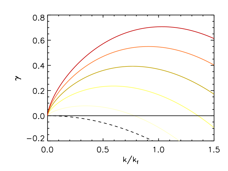
Figure 1: Sketch of the dispersion relation, (15) for different values of velocity shear $S$ (continuous lines with difference colours/grey shades from bottom to top $S=0.5,1.,1.5,2.,2.5$), and (20) (broken line) at the very bottom. Velocity shear and $\gamma$ have dimensions of inverse time and are measured in the units of $u_{\rm rms}k_{\rm f}$.

3.3 Effects of mutual correlations between components of the $\alpha$ tensor

So far we have assumed that only the self-correlations of the components of the $\alpha$ tensor are non-zero and the mutual correlations zero. Let us now generalise (3) to

$$\langle\alpha_{ij}(t)\alpha_{kl}(t^{\prime})\rangle={\mathcal{D}}^{ij}_{kl}\delta(t-t^{\prime}).$$ (24)

Obviously, ${\mathcal{D}}^{ij}_{kl}={\mathcal{D}}^{kl}_{ij}$ and ${\mathcal{D}}^{ij}_{ij}=D_{ij}$. It is again possible to write a closed equation for the first moment of the magnetic field in the form $\partial_{t}\bm{C}^{1}={\sf\bm{N}_{1}}\bm{C}^{1}$ with

$${\sf\bm{N}_{1}}=\left[\begin{array}[]{cc}-k^{2}(\eta_{\rm t}+{\tilde{\eta}}_{yy})&k^{2}{\tilde{\eta}}_{yx}\\ S+k^{2}{\tilde{\eta}}_{xy}&-k^{2}(\eta_{\rm t}+{\tilde{\eta}}_{xx})\end{array}\right]\!,$$ (25)

where

$${\tilde{\eta}}_{yy}={\mathcal{D}}^{yx}_{yx}-{\mathcal{D}}^{yy}_{xx}, {\tilde{\eta}}_{yx}=-{\mathcal{D}}^{yx}_{yy}+{\mathcal{D}}^{yy}_{xy},$$ (26)

$${\tilde{\eta}}_{xy}=-{\mathcal{D}}^{xy}_{xx}+{\mathcal{D}}^{xx}_{yx}, {\tilde{\eta}}_{xx}={\mathcal{D}}^{xy}_{xy}-{\mathcal{D}}^{xx}_{yy}.$$ (27)

This is a generalization of (8). Here, for simplicity, we have assumed $\eta_{xx}=\eta_{yy}=\eta_{\rm t}$ and $\eta_{yx}=\eta_{xy}=0$; in other words the conventional shear–current effect is taken to be zero.

Note that, unlike the self-correlation terms, i.e. ${\mathcal{D}}^{ij}_{ij}$, which must be positive, the mutual correlation terms (e.g., ${\mathcal{D}}^{yy}_{xx}$, or ${\mathcal{D}}^{yx}_{yy}$) can have either sign. Hence, it is a-priori not clear from (25) whether a dynamo is possible or not. However, we note two interesting possibilities below. First, the mutual correlations of the fluctuating $\alpha$ now contribute to off-diagonal components of the turbulent magnetic diffusivity tensor. A dynamo is possible if

$$\frac{S{\tilde{\eta}}_{yx}}{k^{2}\eta_{\rm t}}>1.$$ (28)

Such a dynamo might look deceptively similar to the shear–current dynamo, but is actually not so because in the regular shear–current effect $\eta_{yx}$ emerges due to the presence of shear and hence must be proportional to $S$ for small $S$. Hence for a regular shear–current dynamo we would have $\gamma\sim S^{2}$ and $k^{\rm peak}\sim S$; see BRRK. But here ${\tilde{\eta}}_{xy}$ emerges due to fluctuations of $\alpha$ and may be independent of $S$, at least for small $S$. This would imply that $\gamma\sim S$ and $k^{\rm peak}\sim\sqrt{S}$ but this time even for the first moment of the magnetic field. The growth rate of such a dynamo may however be quite small as it is proportional to ${\tilde{\eta}}_{yx}$ which is the difference between two terms each of which are correlations between different components of the $\alpha$ tensor. Secondly, if ${\mathcal{D}}^{yy}_{xx}>{\mathcal{D}}^{yx}_{yx}$ the fluctuating $\alpha$ effect gives negative contributions to even the diagonal components of turbulent diffusivity, which is reminiscent of the result of Kraichnan (1976).

3.4 Scaling in a simpler zero-dimensional model

The essential physics of (1) and (2) can be captured by an even simpler mean-field model in a one-mode truncation, but with fluctuating $\alpha$ effect, introduced by Vishniac & Brandenburg (1997). Their model, rewritten in our notation and setting all $k$ factors to unity is

$$\partial_{t}\bar{B}_{x} = \alpha\bar{B}_{y}-\eta_{\rm t}\bar{B}_{x},$$ (29)

$$\partial_{t}\bar{B}_{y} = -S\bar{B}_{x}-\eta_{\rm t}\bar{B}_{y}.$$ (30)

This model can be analysed in exactly similar ways. By construction, this model does not have a fluctuating $\alpha^{2}$ effect, and $\alpha$ is a Gaussian random variable with zero mean and covariance

$$\langle\alpha(t)\alpha(t^{\prime})\rangle=D\delta(t-t^{\prime}).$$ (31)

For this model we adopt a more general framework and define the growth-rate of the $p$-th order moment of the magnetic field (the first order is the mean and the second order is the covariance ) to be $p\gamma_{p}$. Explicit calculations, shown in Appendix C, give

$$\gamma_{1}=-\eta_{\rm t},\quad\gamma_{2}=-\eta_{\rm t}+\left(\frac{4DS^{2}}{8}\right)^{1/3}\sim S^{2/3}.$$ (32)

We show in Appendix C that this two-third scaling with shear rate in this zero-dimensional model is equivalent to $\gamma\sim S$ scaling for (1) and (2).

3.5 Possibility of intermittency

We note that (5) and (6) can be considered as coupled stochastic differential equations of the Langevin type but with multiplicative noise. We have taken the probability distribution function (PDF) of the noise to be Gaussian. But, by virtue of multiplicative noise, the PDF of the magnetic field may be non-Gaussian. We have already calculated the first and second moments of this PDF. To probe non–Gaussianity we need to calculate the higher order moments. For (5) and (6) this is a formidable problem. But it is far simpler for the model of Vishniac & Brandenburg (1997). Sokolov (1997) has already argued that the statistics of the magnetic field in the model of Vishniac & Brandenburg (1997) is intermittent; see also Sur & Subramanian (2009). In Appendix C we show that the growth rate for the third and fourth order moments are given by

$$\gamma_{3}=-\eta_{\rm t}+\left(\frac{18DS^{2}}{27}\right)^{1/3}\!\!,\;\;\gamma_{4}=-\eta_{\rm t}+\left(\frac{84DS^{2}}{64}\right)^{1/3}\!\!.\;\;$$ (33)

Clearly, $\gamma_{p}$ has the same scaling dependence on $D$ and $S$, independent of $p$, but nevertheless they are different, i.e., the PDF is non-Gaussian. This non-Gaussianity is best described by plotting

$$\zeta_{p}=\frac{\gamma_{p}+\eta_{\rm t}}{(DS^{2})^{1/3}}$$ (34)

versus $p$ in Fig. 2.

Let us now conjecture that as $p\to\infty$, $\zeta_{p}$ remains finite. Remembering that $\zeta_{1}=0$, the general form would then be

$$\zeta_{p}=\left(\frac{(p-1)(a_{0}+a_{1}p+a_{2}p^{2})}{p^{3}}\right)^{1/3}.$$ (35)

Substituting the form back in (32) and (33) we find $a_{0}=36$, $a_{1}=-30$, and $a_{2}=7$. This formula is also plotted in Fig. 2.

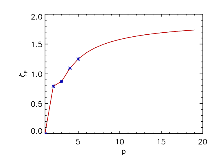
Figure 2: $\zeta_{p}$ versus $p$ as obtained from (34). If the magnetic field had obeyed Gaussian statistics, $\zeta_{p}$ versus $p$ would have been constant.

4 Conclusions

In this paper we have analytically solved a mean-field dynamo model with fluctuating $\alpha$ effect to find self-excited solutions. We have studied the growth rate of different moments (calculated over the statistics of $\alpha$) of the magnetic field. There are three crucial aspects in which our results, the DNS of Yousef et al. (2008), and the analytical results by Heinemann et al. (2011) agree: (a) There is no dynamo for the first moment of the magnetic field, (b) the second moment (mean-square) of the magnetic field shows dynamo action, and (c) the fastest growing mode has a growth rate $\gamma\sim S$ at Fourier mode $k^{\rm peak}\sim\sqrt{S}$. We have further shown that these aspects of our results can even be reproduced by a simpler zero-dimensional mean field model due to Vishniac & Brandenburg (1997). For this simpler model we have also calculated the growth rate for third and fourth order moments and we have explicitly demonstrated the non-Gaussian nature of the PDF of the magnetic field. Given that the incoherent $\alpha$–shear dynamo (often with an additional coherent part) is the most common dynamo mechanism our results provide a qualitative reasoning of why large-scale magnetic fields in the universe may be intermittent. However note also that we have merely shown that the growth rates of the different moments of the magnetic field are different. The eventual nature of the PDF of the magnetic field will also be influenced by the saturation of this dynamo which is outside the realm of this paper. We have also shown that it is possible to find growth of the first moment (mean) of the magnetic field if mutual correlations between different components of the $\alpha$ tensor are assumed to have a certain form (Section 3.3). It will thus be important to check such assumptions from future DNS.

As our paper has been inspired by Heinemann et al. (2011) it is appropriate that we compare and contrast our model and techniques with theirs. Their model consists of the equations of magnetohydrodynamics (MHD) with an external Gaussian, white-in-time force (in the evolution equation for velocity) with the additional assumption that the non-linear term in the velocity equation is omitted. The model thus applies in the limit of Reynolds number $\mbox{Re}\ll 1$. They perform averaging over $xy$-coordinates to obtain mean field equations with an $\alpha$ effect which depends on the helicity averaged over coordinate directions. Our mean field model is derived by first averaging over coordinate directions (standard Reynolds averaging) with the additional assumptions on the statistics (Gaussian, white-in-time) of $\alpha$. Our results are thus not limited by the smallness of the Reynolds number, although all the usual limitations of mean-field theory apply. The assumption of the Gaussian nature of $\alpha$ is well supported by numerical evidence; see Fig. 10 of BRRK. Heinemann et al. (2011) have further used a quasi-two-dimensional velocity field, but this we feel is not an important limitation. They average the first and second moment of the magnetic field over the realisations of force by using cumulant expansion in powers of the Kubo number. As they truncate the expansion at the lowest order in Kubo number it applies to the case of small Kubo number. The most restrictive assumption in our model is the assumption of the white-in-time nature of the $\alpha$ effect. This assumption however allows us to obtain closed equations for all the moments of the magnetic field. The results of Heinemann et al. (2011) is not limited by this assumption. It is interesting to note that, even under the assumption of the white-in-time nature of the $\alpha$ effect, we obtain the same scaling behaviour as Heinemann et al. (2011) and the DNS studies of Yousef et al. (2008).

Here, let us also mention that Kolokolov, Lebedev and Sizov (2011) have recently applied similar techniques to study small-scale kinematic dynamos in a smooth delta-correlated velocity field in the presence of shear to find

$$\gamma_{n}=\frac{3}{2^{5/3}}n^{4/3}D^{1/3}S^{2/3}\sim\lambda n^{4/3},$$ (36)

where $\lambda$ is the expression for the largest Lyapunov exponent describing the divergence of two initially close fluid particles, This Lyapunov exponent was earlier obtained for such flows by Turitsyn (2007). Interestingly, this is exactly the same scaling with shear as in Vishniac & Brandenburg (1997). In the absence of shear the small-scale dynamo can still operate (Chertkov, Kolokolov and Vergassola, 1997) with $\gamma_{n}\sim n^{2}$.

Proctor (2007) have also considered a model similar to ours, although somewhat simpler and more relevant to the solar dynamo, using multiscale expansions. After averaging over the fluctuating $\alpha$ effect, he still finds an effective $\alpha$ effect from which he obtains a dynamo which grows in the mean (as opposed to mean–square in our case). His results give the scaling, $k^{\rm peak}\sim S$ and $\gamma\sim S^{2}$ which disagree with the DNS results of Yousef et al. (2008).

Appendix A Derivation of equations (7) and (8)

It is possible to derive (8) via a method described by Brissaud & Frisch (1974). This method is superior to the one described in Appendix B in the sense that this can be applied even when $\alpha$ is not necessarily white in time, but has (small) non-zero correlation time. On the other hand it is more cumbersome to apply this method to calculate the higher order moments of the PDF of the magnetic field. For the sake of completeness we reproduce below the calculations of Brissaud & Frisch (1974) as applied to our problem.

Let us write symbolically the evolution equations for the mean-field in Fourier space in the following way,

$$\partial_{t}{\mathcal{B}}=\left[{\sf\bm{M}^{\rm d}}+{\sf\bm{M}}\right]{\mathcal{B}}.$$ (37)

Here, ${\mathcal{B}}=(\hat{B}_{x},\hat{B}_{y})$ is a column vector, ${\sf\bm{M}^{\rm d}}$ is the deterministic part of the evolution equations (i.e., the part that depends on $\eta_{ij}$),

$${\sf\bm{M}^{\rm d}}=\left[\begin{array}[]{cc}-k^{2}\eta_{yy}&0\\ S&-k^{2}\eta_{yy}\end{array}\right],$$ (38)

which is also independent of time, and ${\sf\bm{M}}$ is the random part (i.e., the part that depends on $\alpha_{ij}$), with

$${\sf\bm{M}}=ik\left[\begin{array}[]{cc}-\alpha_{yx}&-\alpha_{yy}\\ \alpha_{xx}&\alpha_{xy}\end{array}\right]\equiv ik{\sf\bm{A}}.$$ (39)

To begin, we do not assume that $\alpha$ is white-in-time but that it has finite correlation time $T_{\rm corr}$. Later we shall take the limit of $T_{\rm corr}\to 0$ in a specific way to reach the white-noise-limit. This is equivalent to the regularization in Appendix B

In this section, for simplicity, let us choose our units such that at $t=0$, ${\mathcal{B}}=(1,1)$. In that case the solution to (37) can be easily recast in the integral form

$${\mathcal{B}}(t)=e^{{\sf\bm{M}^{\rm d}}t}+\int_{0}^{t}dt^{\prime}e^{{\sf\bm{M}^{\rm d}}(t-t^{\prime})}{\sf\bm{M}}(t^{\prime}){\mathcal{B}}(t^{\prime}).$$ (40)

Note that we have $\langle{\sf\bm{M}}\rangle=0$ because we have assumed all the components of $\alpha$ to have zero mean. Iterating this equation, we obtain

$$\!\!\!{\mathcal{B}}(t)=e^{{\sf\bm{M}^{\rm d}}t}+\int_{0}^{t}dt^{\prime}e^{{\sf\bm{M}^{\rm d}}(t-t^{\prime})}{\sf\bm{M}}(t^{\prime})e^{{\sf\bm{M}^{\rm d}}t^{\prime}}$$ (41)

$$\!\!\!+\int_{0}^{t}dt^{\prime}\int_{0}^{t^{\prime}}dt^{\prime\prime}e^{{\sf\bm{M}^{\rm d}}(t-t^{\prime})}{\sf\bm{M}}(t^{\prime})e^{{\sf\bm{M}^{\rm d}}(t^{\prime}-t^{\prime\prime})}{\sf\bm{M}}(t^{\prime\prime}){\mathcal{B}}(t^{\prime\prime})$$

$+\mbox{higher order terms}$. Let us also assume that the strength of the fluctuations of $\alpha$ are finite and bounded by $\sigma$. Equation (41) is then an expansion in powers of $\sigma t$. To obtain closed equations for the first moment of the magnetic field, we average (41) over the statistics of $\alpha$ and then take the derivative with respect to $t$. Remembering our earlier notation ${\bm{C}}^{1}\equiv\langle{\mathcal{B}}\rangle$, we obtain

$$\partial_{t}{\bm{C}}^{1}(t)={\sf\bm{M}^{\rm d}}{\bm{C}}^{1}(t)+\int_{0}^{t}dt^{\prime}\langle{\sf\bm{M}}(t)e^{{\sf\bm{M}^{\rm d}}(t-t^{\prime})}{\sf\bm{M}}(t^{\prime}){\mathcal{B}}(t^{\prime})\rangle.$$ (42)

This obviously is not yet a closed equation. To obtain a closure, note that for

$$\sigma(t^{\prime}-s)\ll 1,$$ (43)

from (40), we have

$${\mathcal{B}}(t^{\prime})\approx e^{{\sf\bm{M}^{\rm d}}(t^{\prime}-s)}{\mathcal{B}}(s)+O(\sigma(t^{\prime}-s)).$$ (44)

Substituting (44) in the integrand of the double integral in (42) we obtain the factorization,

$$\langle{\sf\bm{M}}(t)e^{{\sf\bm{M}^{\rm d}}(t-t^{\prime})}{\sf\bm{M}}(t^{\prime})e^{{\sf\bm{M}^{\rm d}}(t^{\prime}-s)}{\mathcal{B}}(s)\rangle\approx$$

$$\langle{\sf\bm{M}}(t)e^{{\sf\bm{M}^{\rm d}}(t-t^{\prime})}{\sf\bm{M}}(t^{\prime})\rangle\langle e^{{\sf\bm{M}^{\rm d}}(t^{\prime}-s)}{\mathcal{B}}(s)\rangle,$$ (45)

if we assume that

$$t^{\prime}-s\gg T_{\rm corr}.$$ (46)

Equations (43) and (46) can both hold only for small Kubo number,

$$K=\sigma T_{\rm corr}\ll 1.$$ (47)

Substituting (45) in (42) and using again (44) we obtain

$$\partial_{t}{\bm{C}}^{1}(t)={\sf\bm{M}^{\rm d}}{\bm{C}}^{1}(t)+\int_{0}^{t}dt^{\prime}\langle{\sf\bm{M}}(t)e^{{\sf\bm{M}^{\rm d}}(t-t^{\prime})}{\sf\bm{M}}(t^{\prime})\rangle{\bm{C}}^{1}(t^{\prime}),$$ (48)

Following Brissaud & Frisch (1974), we shall call this equation the Bourret equation. For small Kubo number we can invert (44) to have

$${\mathcal{B}}(t^{\prime})\approx e^{-{\sf\bm{M}^{\rm d}}(t-t^{\prime})}{\mathcal{B}}(t).$$ (49)

Averaging (49) over the noise we obtain

$${\bm{C}}^{1}(t^{\prime})\approx e^{-{\sf\bm{M}^{\rm d}}(t-t^{\prime})}{\bm{C}}^{1}(t).$$ (50)

Substitute this back into (48), noting in addition that for short-correlated $\alpha$ and $t\gg T_{\rm corr}$, we can replace $\tau\equiv t-t^{\prime}$ in (48) and extend the integral from zero to infinity to obtain

$$\partial_{t}{\bm{C}}^{1}={\sf\bm{M}^{\rm d}}{\bm{C}}^{1}+\int_{0}^{\infty}d\tau\langle{\sf\bm{M}}(\tau)e^{{\sf\bm{M}^{\rm d}}\tau}{\sf\bm{M}}(0)e^{-{\sf\bm{M}^{\rm d}}\tau}\rangle{\bm{C}}^{1},$$ (51)

where we have omitted the $t$ argument on all ${\bm{C}}^{1}(t)$ for brevity. To get this result, remember that the integral above gives negligible contribution for $\tau\gg T_{\rm corr}$ and the matrices ${\sf\bm{M}^{\rm d}}$ and ${\sf\bm{M}}(\tau)$ do not necessarily commute. To go to the white-in-time limit we need to take the limit $\sigma\to\infty$, $T_{\rm corr}\to 0$ in such a way that the product $\sigma^{2}T_{\rm corr}$ remains finite. In this limit the Kubo number goes to zero and the various approximations made above become exact. In this limit the integral in (51) reduces to

$$\partial_{t}{\bm{C}}^{1}(t) = {\sf\bm{M}^{\rm d}}{\bm{C}}^{1}(t)+\langle{\sf\bm{M}}{\sf\bm{M}}\rangle{\bm{C}}^{1}(t)$$ (52)

$$= \left[{\sf\bm{M}^{\rm d}}-k^{2}\langle{\sf\bm{A}}{\sf\bm{A}}\rangle\right]{\bm{C}}^{1}(t).$$

The correlator on the right hand side of (52) can be obtained by using (39) together with (3). This reproduces (8). If instead of (3), (24) is used, (25) can be obtained.

Finally, note that for an $\alpha$ effect which has finite-time-correlations (instead of white-in-time) higher order terms in the expansion in (41) are needed. In such cases it may not even be possible to obtain closed equations like (7).

Appendix B Averaging over Gaussian noise

We explain here another technique used to derive (7) and (8). Let us begin by considering Gaussian vector-valued noise $\nu_{j}(t)$ (not necessarily white-in-time) and an arbitrary functional of that, $F(\bm{\nu})$. Then,

$$\langle F(\bm{\nu})\nu_{j}(t)\rangle=\int dt^{\prime}\langle\nu_{j}(t)\nu_{k}(t^{\prime})\rangle\left\langle\frac{\delta F}{\delta\nu_{k}(t^{\prime})}\right\rangle,$$ (53)

where the average factorises by virtue of the Gaussian property of the noise. Here the operator $\delta(\cdot)/\delta\nu_{k}$ is the functional derivative with respect to $\bm{\nu}$. This useful identity often goes by the name Gaussian integration by parts; see, e.g., Zinn-Justin (1999), Section 4.2 for a proof; see also e.g., Frisch (1996), Frisch & Wirth (1997), or Mitra & Pandit (2004), where this method has been used to derive closed moment equations for the Kraichnan model of passive scalar advection (Kraichnan, 1968).

To obtain an evolution equation for $\bm{C}^{1}=(\langle\hat{B}_{x}\rangle,\langle\hat{B}_{y}\rangle)$ we average each term of (5) and (6) over the statistics of $\alpha_{ij}$. Terms which are product of components of $\alpha_{ij}$ and $\hat{B}_{x}$ or $\hat{B}_{y}$ can be evaluated by using the identity in (53). In particular,

$$\langle\alpha_{yx}\hat{B}_{x}\rangle = \int dt^{\prime}\langle\alpha_{yx}(t)\alpha_{kl}(t^{\prime})\rangle\left\langle\frac{\delta\hat{B}_{x}(t)}{\delta\alpha_{kl}(t^{\prime})}\right\rangle$$ (54)

$$= D_{yx}\frac{\delta\hat{B}_{x}(t)}{\delta\alpha_{kl}(t)}.$$

Here we have considered the magnetic field to be a functional of $\alpha_{ij}$. Substituting the covariance of $\alpha_{ij}$ from (3), integrating the $\delta$ function over time and contracting over the Kronecker deltas, we obtain the last equality in (54).

The functional derivatives of the components of the magnetic field with respect to $\alpha_{ij}$ can be obtained by first formally integrating (5) and (6) to obtain $\hat{B}_{x}(t)$ and $\hat{B}_{y}(t)$, respectively, and then calculating their functional derivatives with respect to $\alpha_{ij}$. We actually need the functional derivative $\delta(\hat{B}_{x}(t))/\delta\alpha_{kl}(t^{\prime})$ and then take the limit $t\to t^{\prime}$. This is a non-trivial step due to the singular nature of the correlation function of $\langle\alpha_{kl}(t)\alpha_{kl}(t^{\prime})\rangle$ as $t\to t^{\prime}$. To get around the difficulty it is possible to replace the Dirac delta function in (3) with a regularised even function and then take limits. We refer the reader to Zinn-Justin (1999), Section 4.2, for a detailed discussion. This regularization is equivalent to using the Stratanovich prescription for the set of coupled SDEs (5) and (6); see, e.g., Gardiner (1994). For reference, all the non-zero functional derivatives needed are given below:

$$\frac{\delta\hat{B}_{x}(t)}{\delta\alpha_{yx}(t)}=-ik\hat{B}_{x}, \frac{\delta\hat{B}_{x}(t)}{\delta\alpha_{yy}(t)}=-ik\hat{B}_{y},$$

$$\frac{\delta\hat{B}_{y}(t)}{\delta\alpha_{xx}(t)}=ik\hat{B}_{x}, \frac{\delta\hat{B}_{y}(t)}{\delta\alpha_{xy}(t)}=ik\hat{B}_{y}.$$ (55)

In particular, since there is no $\alpha_{yy}$ term in (6), we have $\delta(\hat{B}_{y}(t))/\delta\alpha_{yy}(t)=0$, so

$$\left\langle\alpha_{yy}\hat{B}_{y}\right\rangle=D_{yy}\left\langle\frac{\delta\hat{B}_{y}}{\delta\alpha_{yy}}\right\rangle=0.$$

Putting everything together we can now average (5) over the statistics of $\alpha$ to obtain,

$$\partial_{t}\langle\hat{B}_{x}\rangle = -\langle ik\alpha_{yx}\hat{B}_{x}\rangle-\langle ik\alpha_{yy}\hat{B}_{y}\rangle$$ (56)

$$+\eta_{yx}k^{2}\langle\hat{B}_{y}\rangle-\eta_{yy}k^{2}\langle\hat{B}_{x}\rangle$$

$$= -ik(-ik)D_{yx}\langle\hat{B}_{x}\rangle$$

$$+\eta_{yx}k^{2}\langle\hat{B}_{y}\rangle-\eta_{yy}k^{2}\langle\hat{B}_{x}\rangle$$

$$= -(\eta_{yy}+D_{yx})k^{2}\langle\hat{B}_{x}\rangle+\eta_{yx}k^{2}\langle\hat{B}_{y}\rangle.$$

This gives us the first row of the matrix ${\sf\bm{N}_{1}}$ in (8). Applying the same technique to (6), the second row can be obtained.

The same technique can be applied to obtain the matrix ${\sf\bm{N}_{2}}$. Here we end up with evaluating terms of the general form

$$\langle\alpha_{ij}\hat{B}_{k}\hat{B}^{\ast}_{l}\rangle=D_{ij}\left\langle\frac{\delta\hat{B}_{k}}{\delta\alpha_{ij}}\hat{B}^{\ast}_{l}+\hat{B}_{k}\frac{\delta\hat{B}^{\ast}_{l}}{\delta\alpha_{ij}}\right\rangle.$$ (57)

The only non-zero functional derivatives are given in (55). We show the calculation explicitly for the two following examples:

$$\langle\alpha_{yx}{\hat{B}}_{x}{\hat{B}}^{\ast}_{x}\rangle \!\!=\!\! D_{yx}\left\langle\frac{\delta\hat{B}_{x}}{\delta\alpha_{yx}}\hat{B}^{\ast}_{x}+\frac{\delta\hat{B}^{\ast}_{x}}{\delta\alpha_{yx}}\hat{B}_{x}\right\rangle$$ (58)

$$\!\!=\!\! D_{yx}\left[-ik\langle{\hat{B}}_{x}{\hat{B}}^{\ast}_{x}\rangle+ik\langle{\hat{B}}_{x}{\hat{B}}^{\ast}_{x}\rangle\right]=0,$$

and

$$\langle\alpha_{yy}{\hat{B}}_{x}^{\ast}{\hat{B}}_{y}\rangle \!\!=\!\! D_{yy}\left\langle\frac{\delta\hat{B}_{y}}{\delta\alpha_{yy}}\hat{B}^{\ast}_{x}+\frac{\delta\hat{B}^{\ast}_{x}}{\delta\alpha_{yy}}\hat{B}_{y}\right\rangle$$ (59)

$$\!\!=\!\! ikD_{yy}\langle{\hat{B}}_{y}{\hat{B}}^{\ast}_{y}\rangle.$$

Note further that, instead of using the functional calculus above, the same evolution equations for ${\bm{C}}^{1}$ can be obtained by using the technique due to Brissaud & Frisch (1974). This is demonstrated in Appendix A.

Appendix C A zero-dimensional mean-field model with fluctuating $\alpha$

A simpler mean-field model in a one-mode truncation, but with fluctuating $\alpha$ effect, was introduced by Vishniac & Brandenburg (1997); see (29) and (30). For this model we define the following moments of successive orders,

$$\bm{C}^{1} \equiv (\langle\bar{B}_{x}\rangle,\langle\bar{B}_{y}\rangle),$$ (60)

$$\bm{C}^{2} \equiv (\langle\bar{B}_{x}^{2}\rangle,\langle\bar{B}_{y}^{2}\rangle,\langle\bar{B}_{x}\bar{B}_{y}\rangle),$$ (61)

$$\bm{C}^{3} \equiv (\langle\bar{B}_{x}^{3}\rangle,\langle\bar{B}_{x}^{2}\bar{B}_{y}\rangle,\langle\bar{B}_{x}\bar{B}_{y}^{2}\rangle,\langle\bar{B}_{y}^{3}\rangle),$$ (62)

$$\bm{C}^{4} \equiv (\langle\bar{B}_{x}^{4}\rangle,\langle\bar{B}_{x}^{3}\bar{B}_{y}\rangle,\langle\bar{B}_{x}^{2}\bar{B}_{y}^{2}\rangle,\langle\bar{B}_{x}\bar{B}_{y}^{3}\rangle,\langle\bar{B}_{y}^{4}\rangle).$$ (63)

Each of these moments satisfies a closed equation of the form

$$\partial_{t}\bm{C}^{p}={\sf\bm{N}_{p}}\bm{C}^{p}.$$ (64)

The matrices ${\sf\bm{N}_{p}}$ can be found by applying the technique described in Appendix B and by using the covariance of $\alpha$ given in (31). We give below the first four matrices:

$${\sf\bm{N}_{1}}=\left[\begin{array}[]{cc}-\eta_{\rm t}&0\\ -S&-\eta_{\rm t}\end{array}\right],$$ (65)

$${\sf\bm{N}_{2}}=\left[\begin{array}[]{ccc}-2\eta_{\rm t}&2D&0\\ 0&-2\eta_{\rm t}&-2S\\ -S&0&-2\eta_{\rm t}\end{array}\right],$$ (66)

$${\sf\bm{N}_{3}}=\left[\begin{array}[]{cccc}-3\eta_{\rm t}&0&6D&0\\ -S&-3\eta_{\rm t}&0&D\\ 0&-2S&-3\eta_{\rm t}&0\\ 0&0&-3S&-3\eta_{\rm t}\end{array}\right],$$ (67)

$${\sf\bm{N}_{4}}=\left[\begin{array}[]{ccccc}-4\eta_{\rm t}&0&12D&0&0\\ -S&-4\eta_{\rm t}&0&6D&0\\ 0&-2S&-4\eta_{\rm t}&0&2D\\ 0&0&-3S&-4\eta_{\rm t}&0\\ 0&0&0&-4S&-4\eta_{\rm t}\end{array}\right].$$ (68)

The growth rate at order $p$ is defined to be $\bm{C}^{p}\sim\exp(p\gamma_{p}t)$. This gives $\gamma_{1}=-\eta_{\rm t}$, i.e., there is no dynamo. But this also gives dynamo modes with positive eigenvalues given by

$$\gamma_{p}\sim S^{2/3}D_{xx}^{1/3},\quad p=2,3,\ldots$$ (69)

The same result was obtained by Vishniac & Brandenburg (1997) for $\gamma_{2}$ by using a different method.

Note the striking similarity between matrix ${\sf\bm{N}_{2}}$ in (66) and matrix ${\sf\bm{N}_{2}}$ in (10). A trivial way of generalising (66) to one spatial dimension is to replace $D$ and $\eta_{\rm t}$ in (66) by $k^{2}D$ and $k^{2}\eta_{\rm t}$, respectively. The solution of the resultant eigenvalue problem gives the scaling, $\gamma\sim S$ and $k^{\rm peak}\sim\sqrt{S}$. Thus, (66) for this zero dimensional model is equivalent to (10) in the space–time model.

References

- Brandenburg (2005a) Brandenburg A., 2005a, ApJ, 625, 539
- Brandenburg (2005b) Brandenburg A., 2005b, Astron. Nachr., 326, 787
- Brandenburg et al. (2008) Brandenburg A., Rädler K.-H., Rheinhardt M., Käpylä P. J., 2008, ApJ, 676, 740 (BRRK)
- Brissaud & Frisch (1974) Brissaud A., Frisch. U, 1974, J. Math. Phys. 15, 524.
- Cattaneo & Hughes (1996) Cattaneo F., Hughes D. W., 1996, Phys. Rev. E, 54, R4532
- Chertkov, Kolokolov and Vergassola (1997) Chertkov, M., Kolokolov, I., Vergassola, M. 1997, Phys. Rev. E, 56, 5483
- Fedotov et al. (2006) Fedotov S., Bashkirtseva I., Ryashko L., 2006, Phys. Rev. E, 73, 066307
- Frisch (1996) Frisch U., 1996, Turbulence the legacy of A.N. Kolmogorov. Cambridge University Press, Cambridge.
- Frisch & Wirth (1997) Frisch U., Wirth A. 1997, in Boratav O., Eden A., Erzan A., eds, Turbulence Modelling and Vortex Dynamics, Lecture Notes in Physics. Springer, Berlin.
- Gardiner (1994) Gardiner C. W., 1994, in Haken, H., eds, Handbook of stochastic methods for physics, chemistry and the natural sciences. Springer Series in Synergetics, Berlin, Springer.
- Heinemann et al. (2011) Heinemann T., McWilliams J. C., Schekochihin A. A., 2011, Phys. Rev. Lett., 107, 255004
- Hoyng (1987) Hoyng P., 1987, A&A, 171, 357
- Hughes & Proctor (2009) Hughes D. W., Proctor M. R. E., 2009, Phys. Rev. Lett., 102, 044501
- Käpylä et al. (2008) Käpylä P. J., Korpi M., Brandenburg A., 2008, A&A, 491, 355
- Käpylä et al. (2009) Käpylä P. J., Korpi M., Brandenburg A., 2009, ApJ, 697, 1153
- Kazantsev (1968) Kazantsev A. P., 1968, JETP, 26, 1031
- Kleeorin & Rogachevskii (2008) Kleeorin N., Rogachevskii I., 2008, Phys. Rev. E, 77, 036307
- Kolokolov, Lebedev and Sizov (2011) Kolokolov I., Lebedev V., Sizov G., 2011, JETP, 113, 339
- Kraichnan (1968) Kraichnan R., 1968, Phys. Fluids, 11, 945
- Kraichnan (1976) Kraichnan R., 1976, J. Fluid. Mech., 77, 753
- Mitra & Pandit (2004) Mitra D., Pandit R., 2005, Phys. Rev. Lett, 95, 144501
- Moffatt (1978) Moffatt H. K., 1978, Magnetic field generation in electrically conducting fluids. Cambridge Univ. Press, Cambridge, chapter 7.11
- Parker (1955) Parker E. N., 1955, ApJ, 122, 293
- Proctor (2007) Proctor M. R. E., 2007, MNRAS, 382, L39
- Rädler & Stepanov (2006) Rädler K.-H., Stepanov R., 2006, Phys. Rev. E, 73, 056311
- Rogachevskii & Kleeorin (2003) Rogachevskii I., Kleeorin N., 2003, Phys. Rev. E, 68, 036301
- Rüdiger & Kitchatinov (2006) Rüdiger G., Kitchatinov L. L., 2006, Astron. Nachr., 327, 298
- Silant’ev (2000) Silan’tev, N. A., 2000, A&A, 364, 339
- Sokolov (1997) Sokolov D. D., 1997, Astron. Rep., 41, 68
- Sridhar & Subramanian (2009) Sridhar S., Subramanian K., 2009, Phys. Rev. E., 80, 066315
- Sur et al. (2008) Sur S., Brandenburg A., Subramanian K., 2008, MNRAS, 385, L15
- Sur & Subramanian (2009) Sur S., Subramanian K., 2009, MNRAS, 392, L6
- Turitsyn (2007) Turitsyn, K. S., 2007, JETP, 105, 655
- Vishniac & Brandenburg (1997) Vishniac E., Brandenburg A., 1997, ApJ, 584, L99
- Yousef et al. (2008) Yousef T. A., Heinemann T., Schekochihin A. A., Kleeorin N., Rogachevskii I., Iskakov A. B., Cowley S. C., McWilliams J. C., 2008, Phys. Rev. Lett., 100, 184501
- Zinn-Justin (1999) Zinn-Justin J., 1999, Quantum Field Theory and Critical Phenomenon. Oxford University Press, Oxford