Hyperfine characterization and coherence lifetime extension in Pr³⁺:La₂(WO₄)₃

Abstract

Rare-earth ions in dielectric crystals are interesting candidates for storing quantum states of photons. A limiting factor on the optical density and thus the conversion efficiency is the distortion introduced in the crystal by doping elements of one type into a crystal matrix of another type. Here, we investigate the system Pr³⁺:La₂(WO₄)₃, where the similarity of the ionic radii of Pr and La minimizes distortions due to doping. We characterize the praseodymium hyperfine interaction of the ground state (³H₄) and one excited state (¹D₂) and determine the spin Hamiltonian parameters by numerical analysis of Raman-heterodyne spectra, which were collected for a range of static external magnetic field strengths and orientations. On the basis of a crystal field analysis, we discuss the physical origin of the experimentally determined quadrupole and Zeeman tensor characteristics. We show the potential for quantum memory applications by measuring the spin coherence lifetime in a magnetic field that is chosen such that additional magnetic fields do not shift the transition frequency in first order. Experimental results demonstrate a spin coherence lifetime of 158 ms - almost three orders of magnitude longer than in zero field.

I Introduction

Rare-earth ion-doped crystals (REIC) have recently appeared as promising solid state materials for quantum information processing. In the field of quantum computing, achieved milestones include controlled phase gates Longdell et al. (2004) and single qubit arbitrary rotationRippe et al. (2008). While these experimental results were performed on single-qubit and two-qubit systems, scalable schemes have also been poposed Wesenberg et al. (2007). In the field of quantum memories, devices able to faithfully store and release photonic quantum states have been proposed and implemented. Using several different storage-recall protocols Nilsson and Kröll (2005); Afzelius et al. (2009); Hétet et al. (2008); Lauro et al. (2009), high efficiency Hedges et al. (2010), multiple photon storage with large bandwidth Usmani et al. (2010); Bonarota et al. (2011) and entanglement storageClausen et al. (2011); Saglamyurek et al. (2011) were demonstrated in REICs. These results rely on the shielding of the 4f electrons of the rare-earth ions by closed shells, which reduces dephasing by the environment, yielding long coherence lifetimes ($T_{2}$) at liquid helium temperatures. For example, optical coherence lifetimes of 4.4 ms have been observed in Er³⁺:Y₂SiO₅ [Böttger et al., 2009].

Even longer lifetimes have been reported for rare-earth ion hyperfine transitions and accordingly, the qubit in REIC based quantum computing and memories is generally defined by selecting two ground state hyperfine levels. Optical transitions are used to selectively address qubits or to transfer coherences from the optical to the radio-frequency (RF) domain and vice versa. Coherence lifetimes can be extended to 30 s for a ground state hyperfine transition of Pr³⁺:Y₂SiO₅ at liquid helium temperature Fraval et al. (2005). This was achieved in two steps: first, an external magnetic field was applied to the sample in order to decouple one hyperfine transition from magnetic field fluctuations due to host spin flips. As these are the main source of dephasing for Pr³⁺ hyperfine transitions, the zero field coherence lifetime of 500 $\mu$s was extended in this way to 82 msFraval et al. (2004) and later to 860 ms Fraval et al. (2005). The decoupling was achieved by minimizing the transition energy dependence with respect to the magnetic field. This condition is referred as ZEFOZ (Zero First Order Zeeman shift) transitions.Longdell et al. (2006) The coherence lifetime was then further increased by RF decoupling pulses, using a modified version Fraval et al. (2005) of the Carr-Purcell sequence originating from nuclear magnetic resonance.

Y₂SiO₅ is the most thoroughly studied host in REIC quantum information processing. It combines long coherence life times, favored by its low magnetic moment density, mainly due to Y nuclear spins, and high oscillator strengths. A disadvantage of Y-based host material is that doping with Pr³⁺ or Eu³⁺, leads to relatively large inhomogeneous linewidths at high doping concentrations, which limits the maximal achievable optical depth. This is an important concern in high efficiency quantum memories. Tittel et al. (2010) To overcome this limitation for Pr³⁺, we proposed a La-based crystal, La₂(WO₄)₃. Pr³⁺ substitutes La³⁺ in this material, both having very similar ionic radii ($r_{La^{3+}}\,=\,1.18$ Å, $r_{Pr^{3+}}=1.14$ Å) Shannon and Prewitt (1969). Compared to Y₂SiO₅ ($r_{Y^{3+}}=1.02$ Å)Shannon and Prewitt (1969), doping stress is reduced and the inhomogeneous linewidth is 15 times smaller in this compound at high Pr³⁺concentrations. However, the magnetic moment of lanthanum (2.78 $\mu_{B}$) is much higher than that of Y³⁺ (-0.14 $\mu_{B}$) and the La₂(WO₄)₃ magnetic moment density is 7.5 times higher than in Y₂SiO₅. It seems that this should be seriously detrimental to coherence lifetimes but we measured a hyperfine lifetime of 250 $\mu$s by Raman-echoes Guillot-Noël et al. (2009), which is only smaller by a factor of $\approx 2$ compared to the value in Y₂SiO₅. This allowed us to measure narrow and efficient electromagnetically induced transprency in this material. Goldner et al. (2009) This result also suggested that REICs that could be useful for quantum information processing are not limited to the few crystals with very low magnetic moment density. However, since applications require $T_{2}$ values in the ms range, the techniques described above for increasing the coherence lifetime by several orders of magnitude should be used. In this paper, we show that using a ZEFOZ transition, hyperfine $T_{2}$ can reach $158\pm 7$ ms, corresponding to a 630-fold increase. It is therefore possible to strongly reduce the influence of host spin flips even in the case of high magnetic moment density.

ZEFOZ transitions appear at specific magnetic fields (magnitude and direction), which can only be predicted if the system Hamiltonian and all of its parameters are known with high precision. In the present system, the $I=5/2$ nuclear spin of ¹⁴¹Pr (100 % abundance) and the $C_{1}$ site symmetry result in a complicated hyperfine structure. We therefore used the approach of Ref. Longdell et al., 2002, which consists in determining the spin Hamiltonian parameters by coherent Raman-scattering before numerically identifying ZEFOZ transitions. Finally, the coherence lifetimes of the hyperfine transitions were measured by optically detected Raman-echoes.

II Model for the hyperfine interaction

A good approximation for the Hamiltonian of many rare-earth doped compounds is Macfarlane and Shelby (1987)

$$\mathcal{H}_{0}=\left[\mathcal{H}_{FI}+\mathcal{H}_{CF}\right]+\left[\mathcal{H}_{HF}+\mathcal{H}_{Q}+\mathcal{H}_{Z}+\mathcal{H}_{z}\right].$$ (1)

The first two terms, the free ion (including spin-orbit coupling) and the crystal field Hamiltonians determine the energies of the electronic degrees of freedom. The terms in the second bracket, consisting of the hyperfine coupling, the nuclear quadrupole coupling, the electronic and the nuclear Zeeman Hamiltonian, lift the degeneracy of the nuclear spin states.

The site symmetry ($C_{1}$) of our system is low enough that the electronic states are nondegenerate. As a result of this “quenching” of the electronic angular momentum, the electronic Zeeman $\mathcal{H}_{Z}$ and hyperfine interaction $\mathcal{H}_{HF}$ contribute only as second order perturbations. In this approximation, the four last terms of Eq. (1) can be well approximated by a nuclear spin Hamiltonian Teplov (1968):

$$\mathcal{H}_{n} = -g_{J}^{2}\mu_{B}^{2}\vec{B}\cdot\mathbf{\Lambda}\cdot\vec{B}$$

$$-\vec{B}\cdot\left(2A_{J}g_{J}\mu_{B}\mathbf{\Lambda}+g_{I}\mu_{N}\mathbf{E}\right)\cdot\vec{I}$$

$$+\vec{I}\cdot\left(\mathbf{P}-A_{J}^{2}\mathbf{\Lambda}\right)\cdot\vec{I}.$$

Here, $g_{J}$ is the Landé g-value, $\mu_{B}$ the Bohr magneton and $\vec{B}$ the external magnetic field vector. The $\mathbf{\Lambda}$ tensor

$$\Lambda_{\alpha\beta}=\sum_{n=1}^{2J+1}\frac{\langle 0|J_{\alpha}|n\rangle\langle n|J_{\beta}|0\rangle}{E_{n}-E_{0}},$$ (3)

is calculated by second order perturbation theory. $\alpha$ and $\beta$ denote the coordinate axes and the sum runs over the $2J+1$ states of the relevant crystal field multiplet. The crystal field levels of interest in the following are the lowest of the ³H₄ and ¹D₂ multiplets and are written as $|0\rangle$. Other crystal fields levels of each of these multiplets are denoted by $|n\rangle$ and $E_{n}$ represents the energy of that state. $A_{J}$ is the hyperfine constant of the $J$ multiplet, $g_{I}$ is the nuclear $g$-factor, $\mu_{N}$ the nuclear magneton, $\mathbf{E}$ the 3x3 unity matrix and $\vec{I}=\left(I_{x},I_{y},I_{z}\right)$ the vector of nuclear spin operators. $\mathbf{P}$ represents the pure nuclear quadrupole tensor. The operator $(-A_{J}^{2}\vec{I}\cdot\mathbf{\Lambda}\cdot\vec{I})$ has the same form as $\vec{I}\cdot\mathbf{P}\cdot\vec{I}$ and is therefore conventionally referred to as the pseudoquadrupole interaction Baker and Bleaney (1958). We combine these two operators into an effective quadrupole Hamiltonian $\vec{I}\cdot\mathbf{Q}\cdot\vec{I}$. In systems with low site symmetry, as in the present case, the principal axis systems (PAS) of $\mathbf{P}$ and $\mathbf{\Lambda}$ do not coincide in general. The combined operator $\mathbf{Q}$ therefore has again a different PAS.

Considering the first term of Eq. (II), we note that it does not depend on the nuclear spin. It shifts all nuclear spin levels by the same amount and we therefore neglect it in the following. Furthermore, we introduce the abbreviation $\mathbf{M}=-\left(2A_{J}g_{J}\mu_{B}\mathbf{\Lambda}+g_{I}\mu_{N}\mathbf{E}\right)$ for the effective Zeeman coupling tensor. We thus arrive at the following form of the nuclear spin Hamiltonian:

$$\mathcal{H}=\vec{B}\cdot\mathbf{M}\cdot\vec{I}+\vec{I}\cdot\mathbf{Q}\cdot\vec{I}.$$ (4)

The tensors $\mathbf{M}$ and $\mathbf{Q}$ can be parametrized as Macfarlane and Shelby (1987)

$$\mathbf{M}= R_{M}\cdot\left[\begin{array}[]{ccc}g_{x}&0&0\\ 0&g_{y}&0\\ 0&&g_{z}\end{array}\right]\cdot R_{M}^{T}$$ (8)

$$\mathbf{Q}= R_{Q}\cdot\left[\begin{array}[]{ccc}E-\frac{1}{3}D&0&0\\ 0&-E-\frac{1}{3}D&0\\ 0&&\frac{2}{3}D\end{array}\right]\cdot R_{Q}^{T}$$ , (12)

where the $R_{i}=R(\alpha_{i},\beta_{i},\gamma_{i})$ represent rotation matrices and Euler angles, specifying the orientation between $\mathbf{M}$ and $\mathbf{Q}$ tensors PAS ($(x^{\prime},y^{\prime},z^{\prime})$ and $(x^{\prime\prime},y^{\prime\prime},z^{\prime\prime})$ respectively) relative to the laboratory-based reference axis system $(x,y,z)$ (see section III). In general, the $\mathbf{M}$ and $\mathbf{Q}$ principal axes are not aligned and accordingly the $R_{Q}$ and $R_{M}$ matrices are not identical. The nuclear spin Hamiltonian of a given crystal field level therefore depends on 11 parameters: $g_{x},g_{y},g_{z},\alpha_{{M}},\beta_{{M}},\gamma_{{M}},D,E,\alpha_{{Q}},\beta_{{Q}},\gamma_{{Q}}$.

In zero magnetic field, the quadrupole interaction results in a partial lifting of the nuclear spin states degeneracy. The corresponding structures for the ³H₄ and ¹D₂ levels was determined by holeburning experiments Guillot-Noël et al. (2007, 2009) and are shown in Fig. 1. We label the levels by their projections onto the $z^{\prime\prime}$ principal axes of the $\mathbf{Q}$ tensor, noting that these states are not eigenstates of the nuclear spin Hamiltonian. Since the PAS of the $\mathbf{Q}$ tensors of different crystal field levels do not coincide, their quantization axes are also different. For the small magnetic fields used to determine spin Hamiltonian parameters, the hyperfine structure remains close to the zero field one, which allows us to identify resonance lines with transitions between zero-field states.

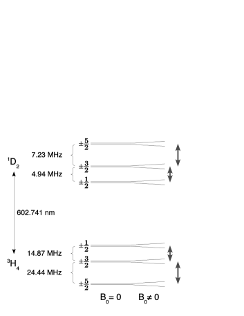
Figure 1: Optical transition and hyperfine level structure of Pr³⁺:La₂(WO₄)₃. The order of the energy levels follows from previous work Guillot-Noël et al. (2009), whereas the transition frequencies could be measured with higher precision utilizing zero field Raman-heterodyne scattering within the present work. The arrows on the right indicate the range of hyperfine transitions excited by RF in the separate experiments.

III Experiment

We used Raman-heterodyne scattering (RHS) to obtain hyperfine spectra of both, the electronic ground state and the electronically excited state. RHS is a magneto-optic double resonance technique, that requires a laser and an RF field Mlynek et al. (1983); Wong et al. (1983). The laser light has multiple functions in the scheme. The first is to prepare a population difference between the hyperfine levels by optical pumping or transfer to auxiliary states. If the RF field is resonant with the hyperfine transitions, it creates coherences between those states, which are transferred to coherences in optical transitions by the light. These optical coherences represent electronic dipoles, which act as a source of a new optical field that is shifted by the RF frequency with respect to the incident laser frequency - the Raman-field. As this field is emitted in the same optical mode as the incident light, it can be measured by optical heterodyne detection, using the transmitted laser beam as the local oscillator.

We used a sample of high optical quality, grown by the Czochralski method, containing 0.2% at. Pr³⁺. The 5x5x5 mm crystal was mounted in an optical cryostat and cooled to liquid helium temperatures. La₂(WO₄)₃ forms a monoclinic crystal with a $C2/c$ space group, identical to that of Y₂SiO₅. The La³⁺ ions occupy only one crystallographic site of $C_{1}$ symmetry. In each unit cell (containing 4 formula units), this site appears at 8 positions which are related by inversion, translation and $C_{2}$ symmetries. The $C_{2}$ axes are identical to the $C_{2}$ crystal symmetry axis, also denoted by $b$ in the following. The $C_{2}$ symmetry divides the La positions into two groups of 4 ions, which behave differently, unless the magnetic field is perpendicular or parallel to the $b$ axis. These two groups are called sub-sites in the following. The crystal surfaces where polished perpendicular to the $(X,Y,Z)$ principal axes of the optical indicatrix. Optical back reflection at the $Z$-surface and mechanical alignment of the X and Y surfaces was used to align the crystal along our reference $(x,y,z)$ axes, defined by the static magnetic field coils (see below). Apart from alignment errors the $(X,Y,Z)$ axes should be a replica of $(x,y,z)$, the laser propagating along $Z$ and the $b$ axis expected to be closely aligned to the laboratory frame $y$ axis.

A Coherent 899-21 dye laser, further stabilized by home-built electronics with respect to intensity and frequency (linewidth $<$ 20 kHz), served as light source. It was tuned to a wavelength of 602.741 nm (vac.), corresponding to the center of the transition involving the lowest energy crystal field levels of the ³H₄ and ¹D₂ multiplets (see Fig. 1). Typical powers for the scattering/heterodyne light were 0.3 to 2 mW focused, from a collimated beam of 1.5 mm diameter, with a 300 mm lens into the sample. We generated the optical pulses and frequency chirps by double pass acousto-optic modulator setups.

The RF fields were applied to the sample by a 10 turn 6 mm diameter coil. For continuous wave experiments (ground state), one side of the coil was terminated by a 50 $\Omega$ load, the other was attached to an RF driver running at a power level of 1 W.

For the exited state spectra, we used a pulsed RHS scheme. Here the coil was part of an appropriate tuned tank-circuit and typical RF powers were 250 W, resulting in maximum signal amplitudes for RF-pulse durations of 3-4 $\mu$s. Figure 2 shows the sequences used for the two types of experiments.

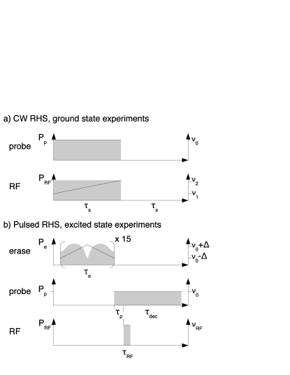
Figure 2: Pulse sequences. Black lines indicate frequencies and grey areas the applied optical/RF powers.
a) CW (continuous wave) sequence for the ground state measurements. A low power laser probe ($P_{p}$ = 0.3 mW) and a scanning frequency RF ($P_{RF}\approx$ 1 W, $\nu_{1}$ = 7.4 and $\nu_{2}$ = 22.4 MHz for $\left|\pm\frac{1}{2}\right>\leftrightarrow\left|\pm\frac{3}{2}\right>$ or respectively 17.1 and 32.1 MHz for $\left|\pm\frac{3}{2}\right>\leftrightarrow\left|\pm\frac{5}{2}\right>$) were applied to the sample to detect the spectra on the frequency encoded time-scale ($\tau_{s}$ = 50 ms). The optimum temperature of the cold finger for this scheme was 4.5 K, since still lower temperatures gave such slow hyperfine level relaxation rates that it would be necessary to repump the hyperfine level population.
b) Pulsed RHS-sequence for the excited state. Probe and erase beam were overlapped in the sample at angle of 0.6^∘. To allow for higher repetition rate the chirped erase laser ($\Delta$ = 64 MHz, $\tau_{e}$ = 10 ms, $P_{e}$ = 8-30 mW due to the frequency dependence of the AOM) redistributed the populations. Initial hyperfine population was created by the probe beam ($P_{p}$ = 1.2 mW, $\tau_{p}$ = 100 $\mu$s) and converted to coherences by an RF pulse ($\nu_{RF}$ = 4.94/7.23 MHz ($\left|\pm\frac{1}{2}\right>\leftrightarrow\left|\pm\frac{3}{2}\right>$ resp. $\left|\pm\frac{3}{2}\right>\leftrightarrow\left|\pm\frac{5}{2}\right>$), $P_{RF}$ = 214/287 W, $\tau_{RF}$ = 4 $\mu$s). For optical heterodyne detection the same probe beam was left active for an additional time $\tau_{dec}$. The temperature of the cold finger for this scheme was 2.4 K.

The frequencies for the RF excitation and the shifting of the laser frequency were generated by 48 bit / 300 MHz direct digital synthesizers. We controlled the timing of the pulses and frequency-chirps by a wordgenerator with a resolution of 4 ns. Detection of the heterodyne beat signal was accomplished by a 100 MHz balanced photo receiver (Femto HCA-S), a phase sensitive quadrature-detection demodulation scheme, appropriate analog and digital filters and a digital oscilloscope.

The static magnetic field was created by a set of three orthogonal Helmholtz coil pairs. They are mounted outside the cryostat and their coil-diameters range from 20 to 40 cm, providing a homogeneous field over the sample volume in their center. With currents of about 10 A, each coil pair generates a static magnetic field of about 8 mT. To control the field vector a computer control was set up for the current sources of the Helmholtz coils. To compensate non-linearities and drifts, we used a set of three orthogonal Hall probes as sensors for a computer-based feedback loop. The absolute error of the field components is $<0.06$ mT and the relative linear error for the static magnetic field is $<0.3\%$. To minimize the effect of small background fields (e.g. earths magnetic field) a small compensation field was used, which minimized the observed zero-field RHS line splitting and also led to almost perfect destructive interference Mitsunaga et al. (1984, 1985). We used this compensation field as our zero-field reference in all measurements.

For an optimal determination of the Hamiltonian parameters, it is important to sample different strengths and orientations of the magnetic field. In our experiments, we used a spiral on the surface of an ellipsoid Longdell et al. (2002):

$$\vec{B}(t)=\left(\begin{array}[]{c}B_{x}\sqrt{1-t^{2}}\cdot\cos\left(6\pi t\right)\\ B_{y}\sqrt{1-t^{2}}\cdot\sin\left(6\pi t\right)\\ B_{z}\cdot t\end{array}\right).$$ (16)

Here, we use

$$t=-1+\left(N-1\right)\frac{2}{N_{tot}-1},\quad N=1,2,...,N_{tot}.$$

to represent the discrete coordinate along the trajectory. For the ground state series, we measured $N_{tot}=$ 101 orientations, with magnetic field amplitudes $[B_{x},B_{y},B_{z}]=[7,9,8]$ mT and for the excited state we used $N_{tot}=$ 251 and $B_{x}=B_{y}=B_{z}=6.5$ mT. Figure 3 shows some typical experimental spectra for the ground- and excited state.

Figure 3: (Color online) Representative ground state CW RHS and exited state pulsed RHS spectra. Both spectra from the ground state ($\left|g,i\leftrightarrow j\right>$) are recorded at $N=15$, corresponding to $\vec{B}=(2.60,-5.27,-5.76)$ mT. For the excited state spectra, we used $N=211$, corresponding to $\vec{B}=(4.62,1.19,4.42)$ mT. The normalization is relative to the largest line from ground or excited state spectra, respectively. The ground state spectra shown here resolve all 8+8 possible RHS transitions, while in the excited state spectra not all lines are resolved. The histograms on the right show the distributions of fitted full width at half maximum (FWHM) RHS-linewidths for all recorded data (see Section IV.1), plotted separately for the two hyperfine transitions ($\left|g/e,i\leftrightarrow j\right>$, $i/j=\pm\frac{1}{2}/\pm\frac{3}{2}$ or $\pm\frac{3}{2}/\pm\frac{5}{2}$). For both, the ground and the excited state, the $\pm\frac{3}{2}\leftrightarrow\pm\frac{5}{2}$ linewidths are bigger (see Section V.3). The mean linewidths are $\left|g,\pm\frac{1}{2}\leftrightarrow\pm\frac{3}{2}\right>\approx$ 105 kHz, $\left|g,\pm\frac{3}{2}\leftrightarrow\pm\frac{5}{2}\right>\approx$ 301 kHz, $\left|g,\mbox{all}\right>\approx$ 196 kHz and $\left|e,\pm\frac{1}{2}\leftrightarrow\pm\frac{3}{2}\right>\approx$ 18.3 kHz, $\left|e,\pm\frac{3}{2}\leftrightarrow\pm\frac{5}{2}\right>\approx$ 26.3 kHz, $\left|e,\mbox{all}\right>\approx$ 22.3 kHz.

IV The fitting procedure

In the case of Pr³⁺:La₂(WO₄)₃, 11 spin Hamiltonian parameters are necessary ($D$, $E$, $g_{x,y,z}$, $(\alpha,\beta,\gamma)_{Q/M}$) to compute the line positions of excited or ground state spectra for an arbitrary external magnetic field. These calculations have to take into account the magnetically non-equivalent Pr³⁺ sites, which are related by the crystal $C_{2}/b$ axis, corresponding to the $Y$-direction of the crystal’s optical indicatrix axis system $(X,Y,Z)$. As this system may not be perfectly aligned to the laboratory reference system $(x,y,z)$ (see section III), $(\alpha,\beta)_{C_{2}}$ angles give the $C_{2}$ orientation with respect to the $x$ and $z$ axes. This gives a total of 13 parameters that are to be extracted from the recorded series of spectra.

IV.1 Source data

While it is possible to calculate directly the spectra from the Hamiltonian, the resulting amplitudes and phases do not agree with the experimentally observed values, since they depend strongly on experimental details, such as cable lengths, tuning curves etc. By far the most precise parameters of the spectra are the positions of the resonance lines. We therefore extracted these in a first step and used only the resonance frequencies as input to the actual fitting procedure.

For the extraction of the line positions, we fitted the absolute-value representation of the measured spectra to a series of gaussian-shaped resonance lines. To discriminate between real lines and noise or artifacts, we considered additional parameters like peak height, line width and noise level. For most of the recorded data the procedure worked satisfyingly, even for partially overlapping resonance lines. The positions of lines that had very small amplitudes or could not be fitted well due to strong overlapping were identified visually or omitted.

IV.2 Fitting of Hamiltonian parameters

After determining the resonance line positions, we fitted the Hamiltonian parameters such that the resulting line positions agreed with the experimental data. Due to the large number of parameters and their complicated interdependency, gradient-based algorithms are not efficient, as they tend to stick to local minima. In our case, the combination of first running a probabilistic and then a direct search yielded the best convergence to the global minimum. As in the work of Longdell Longdell et al. (2002, 2006) we used simulated annealing Kirkpatrick et al. (1983) for the first step. When the preliminary results of this step appeared to converge towards a global minimum, we switched to a pattern search algorithm Audet and Dennis (2003), which polls meshes of adjacent points to find a better minimum. This reduced the necessity for an excessively long search at low temperatures in the simulated annealing procedure and represents an additional check for the quality of the minimum.

The implemented algorithm minimizes the root mean square (RMS) deviation between the measured and the calculated line positions of all spectra,

$$f^{RMS}_{k}=\sqrt{\sum_{N=1}^{N_{tot}}\frac{\sum_{i=1}^{Q_{N}}\left(\nu^{exp}_{iN}-\nu^{k}_{iN}\right)^{2}}{Q_{N}}}.$$

For each of the $N_{tot}$ spectra $Q_{N}$ line pairs, consisting of the measured frequencies $\nu^{exp}_{iN}$ and the corresponding calculated frequencies $\nu^{k}_{iN}$ were identified. The index $i$ runs over all lines in a single spectrum. Accordingly all possible eigenvalue differences ($\nu^{k}_{iN}$) for the given Hamiltonian, derived from Eq. (4) using the given set of parameters of the $k^{th}$ iteration and the $N^{th}$ magnetic field orientation (Eq. (16)), were calculated. Not all possible lines are always resolved or visible in the spectra (see e.g. Fig. 3). Therefore, we matched theoretical to experimental lines by minimizing the absolute deviations for this spectrum; each experimental line was associated only with a single theoretical line. Lines that could not be assigned uniquely were not considered in that step of the fitting procedure. This mapping could change during the fitting procedure, but in the final steps of the search, the procedure resulted in an unambiguous assignment.

We initialized the simulated annealing algorithm with a random guess for the parameters. At each following iteration one of the Hamiltonian parameters was randomly chosen and varied in an interval determined by the current temperature. If the variation resulted in a new minimum value of the RMS error ($f^{RMS}_{best}$), the new point was always accepted. If the variation was higher than the previous minimum, the algorithm calculated the Boltzman factor

$$p_{k}=\exp\left(\frac{-\left(f^{RMS}_{k}-f^{RMS}_{best}\right)}{k_{B_{l}}\cdot T_{k_{l}}}\right)$$ (17)

and compared it to a random number $p_{r}$ $\epsilon$ $\left[0,1\right]$. The new point was accepted for $p_{k}>p_{r}$ and rejected otherwise. The RMS misfits $f^{RMS}_{k}$ and $f^{RMS}_{best}$ represent the deviation of the current iteration and the best observed deviation of all previous iterations, respectively. The temperatures $T_{k_{l}}$ are defined in the individual $l$-th parameter units. Conversion factors $k_{B_{l}}$ ensured correct units and parameter independent scaling of the denominator in Eq. (17). All temperatures were lowered continuously as the fitting improved. This was done for all $T_{k_{l}}$ in the same way, so that for simplicity we may speak in terms of a global temperature and omit the $l$-index where it is not necessary. At high temperatures the algorithm sampled a large parameter range. Enabling it to resettle in states of slightly higher misfits enables the algorithm to trace a large search-space and to avoid getting stuck in a local minima at the same time. As the temperature was gradually lowered, the parameter values became more confined in the vicinity of the global minimum.

The whole procedure was implemented as a MATLAB program, utilizing the Global Optimization Toolbox functions patternsearch and simulannealbnd.

IV.3 Restrictions and Model

We chose the initial temperature $T_{0}$ such that the corresponding changes of the line positions were $\approx 10$ times the inhomogeneous line widths. Typically $k_{max}\approx 10^{6}$ iterations for the simulated annealing lead to reliable results. Within the first 80% of the iterations the temperature was gradually lowered as $T_{k}\approx T_{0}\left(1-k/k_{max}\right)^{2}$. Then $T_{k}$ was left constant at a value corresponding to a frequency uncertainty of a fraction of the typical line-widths (a few kHz).

During the whole fit, the parameters were constrained. As values for $D$ and $E$ can be derived from hole-burning experiments Guillot-Noël et al. (2007, 2009) their boundaries were restricted to $\pm$10% of the literature values. For the gyromagnetic ratios, the boundaries were chosen to $\pm$100% of the expected values of -(10-100) MHz/T observed in similar systems.Macfarlane and Shelby (1987); Longdell et al. (2002) The Euler angles were allowed to vary over the whole definition range. The probability for choosing a specific parameter for the variation was proportional to the (relative) size of its boundaries. As indicated above, the new value of this parameter was chosen by adding a random value out of the interval $\pm T_{k_{l}}$. If the new value did not lie within the boundaries, the process was repeated. The final direct search was set up with the same boundaries and typically terminated after $5\cdot 10^{4}$ iterations.

The orthogonal axes of the B-field coils define the reference coordinate system $(x,y,z)$. Euler-angles and transformations refer to this basis and are given in “zyz”-convention Goldstein et al. (2002) (see. Eq. (24) for details). As indicated before, we did not constrain the relative orientation of the quadrupole $\mathbf{Q}$- and Zeeman $\mathbf{M}$-tensor. To avoid ambiguous results, we fitted all measured spectra of a single electronic state simultaneously. Due to the two non-equivalent sites this results in a maximum of 16 lines per spectrum.

Since the assignment of the resonance lines to the two sites is not known, we had to fit both sites simultaneously. Instead of fitting $2\cdot 11=22$ parameters, we used the fact that they are related by a $C_{2}$ rotation. Using Eq. (4) for site 1, we write the Hamiltonian for site 2 as

$$\mathcal{H}_{2} = \vec{B}\cdot\left(R_{C_{2}}\mathbf{M}_{1}R_{C_{2}}^{T}\right)\cdot\vec{I}+\vec{I}\cdot\left(R_{C_{2}}\mathbf{Q}_{1}R_{C_{2}}^{T}\right)\cdot\vec{I},$$

with

$$R_{C_{2}}=R_{C}^{T}\cdot R_{\pi}\cdot R_{C},$$

$$R_{C}=R\left(\alpha_{C_{2}},\beta_{C_{2}},0\right),\quad R_{\pi}=R\left(180^{\circ},0,0\right).$$

The angles $\alpha_{C_{2}}$ and $\beta_{C_{2}}$ correspond to the spherical coordinates of the $C_{2}$ axis in the laboratory system.

V Results

The underlying symmetry of the crystal field and the structure of the spin Hamiltonian cause some ambiguity if only RHS spectra are used to determine the Hamiltonian parameters. The thesis of J. Longdell Longdell (2003) provides a detailed review of relevant symmetries that make it impossible to unambiguously determine all Hamiltonian parameters from RHS spectra alone. Important for our investigation is the fact that the RHS spectra do not depend on the signs of $D$, $E$ and the gyromagnetic factors $g_{x}$, $g_{y}$ and $g_{z}$. In addition, different sets of Euler angles correspond to the same tensor orientations. As a consequence, different runs with random initial values lead to apparently different solutions. We checked that these solutions are related by the symmetry operations mentioned above and verified thus that we really found a unique global minimum.

V.1 Electronic ground state

Figure 4 shows the experimental data for $N_{tot}=101$ different external magnetic fields.

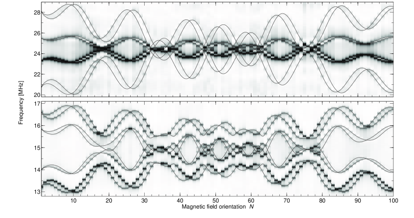
Figure 4: Ground state $\left|\pm\frac{1}{2}\right>\leftrightarrow\left|\pm\frac{3}{2}\right>$ and $\left|\pm\frac{3}{2}\right>\leftrightarrow\left|\pm\frac{5}{2}\right>$ hyperfine transition CW RHS spectra. The solid lines represent the fit results and the shaded background the absolute value of the experimental spectra. For each field orientation, the spectrum was normalized to the maximum signal amplitude.

Several fit trails reliably led to the parameters shown in Table 1 and represented by the solid lines in Fig. 4.

Table 1: Ground state spin Hamiltonian parameters

parameter	value	fit error	unit
D	-6.3114	0.0027	MHz
E	-0.8915	0.0021	MHz
$\alpha_{Q}$	20.4	3.3	deg.
$\beta_{Q}$	147.7	1.4	deg.
$\gamma_{Q}$	10.2	1.4	deg.
$g_{x}$	-51.7	3.6	MHz/T
$g_{y}$	-23.5	1.1	MHz/T
$g_{z}$	-146.97	0.75	MHz/T
$\alpha_{M}$	30.1	3.8	deg.
$\beta_{M}$	146.59	0.55	deg.
$\gamma_{M}$	13.09	0.69	deg.
$\alpha_{C_{2}}$	88.34	0.47	deg.
$\beta_{C_{2}}$	92.45	0.31	deg.

With these parameters, the RMS deviation between all accounted line positions and the fit is $\approx 32$ kHz, significantly smaller than the average linewidth of the ground state RHS lines of $\approx 196$ kHz (see Fig. 3), indicating that it is dominated by statistical error. At the end of the fitting procedure, $L=$1218 of the total 1221 experimental lines from $N_{tot}=101$ spectra could be assigned to calculated resonance line positions. To estimate the uncertainty of the fitted parameters, we sampled the parameter space in the vicinity of the global minimum by repeating the probabilistic part of the fitting procedure again using a fixed, low temperature. Such a procedure can be shown to be rigorous if the only source of error is gaussian noise in the line positions. Longdell et al. (2002); Longdell (2003) As an estimation for the noise in the line positions we used the mean ratio of fitted line widths $\sigma_{i}$ to the individual signal to noise (SNR_i) for all contributing RHS-lines:

$$\nu_{\sigma}=\frac{1}{L}\sum^{L}_{i}\frac{\sigma_{i}}{\mbox{\it SNR\rm}_{i}}.$$

For the ground state data we found $\nu_{\sigma}=$ 1.4 kHz. According to this we chose the fixed temperature $T_{\sigma}$, so that a single parameter change from its optimum value by $T_{\sigma_{l}}$ resulted in an increase of the RMS deviation by $\nu_{\sigma}$. After $2\cdot 10^{6}$ iterations the histograms of the accepted parameters all showed a gaussian shape, whose $1\sigma$-width are given as fit error in Table 1.

Apart from the statistical error, we also consider systematic errors. The most important contribution is due to the calibration error of the magnetic field. We estimate its precision to $\approx 0.65\%$, which translates to the same fractional uncertainty of the gyromagnetic ratios $g_{x}$, $g_{y}$ and $g_{z}$. As the parameters are given in the laboratory-fixed reference frame $(x,y,z)$ a misalignment of the crystal does not contribute to the error but is expressed by the $\alpha_{C_{2}}$ and $\beta_{C_{2}}$ values. They determine the orientation of the $C_{2}$ axis and therefore also that of the optical indicatrix $(X,Y,Z)$ in our laboratory frame. The only systematic contribution in the angles arise from non-orthogonality of the coils, which is $<1^{\circ}$. The uncertainty of the alignment of the crystal relative to our reference $(x,y,z)$ and that of the crystal surfaces to the optical indicatrix $(X,Y,Z)$ results in an error of $\approx 5^{\circ}$ for the angles seen relative to the crystal axis system. The frequency scan was generated by direct digital synthesis, resulting in negligible uncertainty in the frequency scale.

V.2 Excited state

For the excited state we used the same procedure as for the ground state. With the optimal fit parameters, we found an RMS deviation of 3.1 kHz between theoretical and experimental frequency values, using $L=$ 2345 of the 2353 measured lines in $N_{tot}=251$ spectra. Compared to the mean experimental FWHM of 22.3 kHz, the RMS deviation is even better than for the ground state. We mainly attribute this to the higher quality of pulsed RHS spectra, with fewer line shape artifacts. Figure 5 and Table 2 show the results.

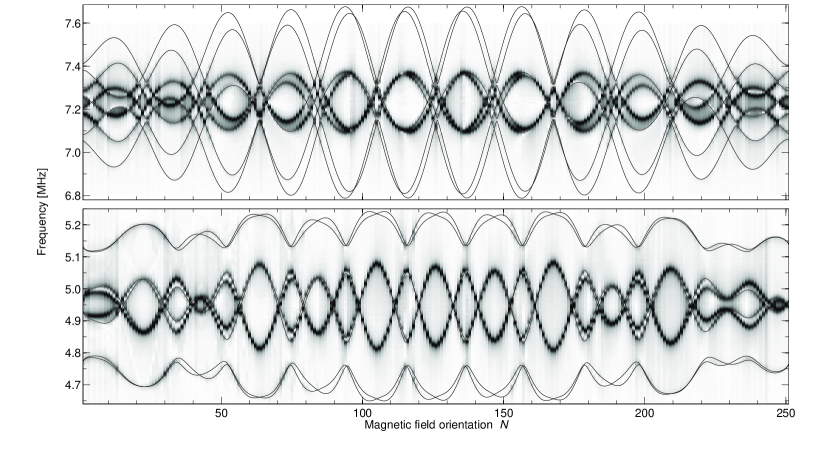
Figure 5: Excited state $\left|\pm\frac{1}{2}\right>\leftrightarrow\left|\pm\frac{3}{2}\right>$ and $\left|\pm\frac{3}{2}\right>\leftrightarrow\left|\pm\frac{5}{2}\right>$ hyperfine transition pulsed RHS spectra. The solid lines represent the fit results and the shaded background the absolute value of the experimental spectra. For each field orientation, the spectrum was normalized to the maximum signal amplitude.

Table 2: Excited state spin Hamiltonian parameters

parameter	value	fit error	unit
D	1.90705	0.00023	MHz
E	0.35665	0.00014	MHz
$\alpha_{Q}$	-18.51	0.71	deg.
$\beta_{Q}$	73.83	0.48	deg.
$\gamma_{Q}$	-84.22	0.37	deg.
$g_{x}$	-17.22	0.27	MHz/T
$g_{y}$	-14.39	0.10	MHz/T
$g_{z}$	-18.37	0.14	MHz/T
$\alpha_{M}$	-23.7	2.4	deg.
$\beta_{M}$	88.5	4.1	deg.
$\gamma_{M}$	-80.1	1.8	deg.
$\alpha_{C_{2}}$	88.63	0.25	deg.
$\beta_{C_{2}}$	92.69	0.24	deg.

For the determination of the fit errors, we used the same procedure as for the ground state. The average uncertainty of the line positions was $\nu_{\sigma}=$ 136 Hz. The systematic errors are again dominated by the calibration error of the magnetic field. Although the crystal was remounted between the excited and ground state experiments, the resulting orientation of the $C_{2}$ axis agrees between the two data sets within less than one degree, which is less than our alignment accuracy. As the Zeeman tensor is almost axially symmetric, $g_{x}\approx g_{z}$, its orientation relative to the quadrupole tensor or to the ground state tensor orientations can not be completely determined.

V.3 Discussion

Examining Tables 1 and 2, it appears that the principal values for the $\mathbf{Q}$ and $\mathbf{M}$ tensors are similar to those found in other hosts like Y₂SiO₅Longdell et al. (2002), LaF₃ or YAlO₃ Macfarlane and Shelby (1987). Especially, the ground state gyromagnetic tensor is anisotropic with one large component, in contrast to the excited state which also exhibits smaller values. To get some insight into these properties, we compared these results with calculations derived from crystal field calculations.

In a previous work Guillot-Noël et al. (2010), we found that quadrupolar $D$ and $E$ values for ground and excited states (see Eq. (12)) could be very well reproduced starting from electronic wavefunctions obtained by a crystal field analysis. The latter was done assuming a $C_{2v}$ site symmetry, which is higher than the actual one ($C_{1}$). In this higher symmetry, the $\mathbf{Q}$ tensors for different crystal field levels are colinear, in clear contradiction with our results. Nevertheless, it seems that the additional crystal field parameters of $C_{1}$ symmetry have little effects on the $\mathbf{Q}$ principal values. In the following, we present the calculations of the $\mathbf{M}$ tensor principal values.

In $C_{2v}$ orthorhombic symmetry, the spin Hamiltonian of Eq. (4), expressed in the $(x_{c},y_{c},z_{c})$ crystal field axes, reads:

$$\mathcal{H^{\prime\prime}}=\sum_{i=x_{c},y_{c},z_{c}} B_{i}g_{i}I_{i}$$ (18)

$$+D({I^{2}_{z_{c}}}-\frac{I\left(I+1\right)}{3})+E({I^{2}_{x_{c}}}-{I^{2}_{y_{c}}})$$

where the $g_{i}$ are related to the $\mathbf{\Lambda}$ tensor by (see Eq. (II)):

$$g_{i}=-2A_{J}g_{J}\mu_{B}\Lambda_{ii}-g_{I}\mu_{N}.$$ (19)

The $\mathbf{\Lambda}$ tensor is given by Eq. (3) and can be calculated from the electronic wavefunctions. The latter were found using a free ion and crystal field Hamiltonian whose parameters were fitted to experimentally determined crystal field levels Guillot-Noël et al. (2010). In this calculation, we use arbitrary permutations of the $(x_{c},y_{c},z_{c})$ axes. This results in different sets of $E$,$D$ values which give the same hyperfine energy levels. We subsequently fix the choice of the axis system such that the convention $0\leq 3E/D=\eta\leq 1$ [Abragam, 1994] is fulfilled, thereby resolving ambiguous sets of parameters, such as (in MHz) $D=2.082,E=-3.3445$ and $D=-6.0578,E=-0.6313$, which describe identical ground state zero field hyperfine structures and correspond to an exchange of $x_{c}$ with $z_{c}$. With this convention, we fix the permutation of the axes and thus the values for $D$ and $E$ for both electronic states. The crystal field parameters we used and the corresponding $E$ and $D$ values for the ground and excited states are listed in Table 3. The electronic wavefunction of the excited ¹D${}_{2}(\left|1\right>)$ level is used instead of that of ¹D${}_{2}(\left|0\right>)$ to take into account a wrong ordering in the calculated crystal field levels of this multiplet Esterowitz et al. (1979); Guillot-Noël et al. (2010).

Table 3: Crystal field parameters $B_{ij}$, calculated $\mathbf{Q}$ and $\mathbf{M}$ tensor principal values and second order hyperfine interaction parameters.

$B_{ij}$	(cm-1)		ground state	excited state	unit
$B_{20}$	375	$D$	-6.1	2.0	MHz
$B_{22}$	-93	$E$	-0.63	0.30	MHz
$B_{40}$	768	$g_{x_{c}}$	-32	-18	MHz/T
$B_{42}$	445	$g_{y_{c}}$	-22	-4	MHz/T
$B_{44}$	1027	$g_{z_{c}}$	-151	-18	MHz/T
$B_{60}$	267	$A_{J}$	937	697	MHz
$B_{62}$	-402	$g_{J}$	0.81	1.03
$B_{64}$	-61	$\Lambda_{x_{c}x_{c}}$	0.0280	0.0066	cm
$B_{66}$	-52	$\Lambda_{y_{c}y_{c}}$	0.0140	-0.0090	cm
		$\Lambda_{z_{c}z_{c}}$	0.2000	0.0069	cm

Comparing Tables 1 and 2 with Table 3 shows that a reasonable agreement is found between experimental and calculated principal values of ground and excited state $\mathbf{M}$ tensors. Again this suggests that additional parameters appearing in calculations using $C_{1}$ symmetry mainly determine the relative orientation between the different tensors. Calculated values especially reproduce two features mentioned above: the very large value of $g_{z}$ for the ground state and the smaller $g_{i}$ values for the excited state compared to the ground state. A qualitative understanding of these properties can be obtained from the crystal field analysis by looking at the different factors entering in Eq. (19). They are summarized in Table 3. We first note that the isotropic and crystal field independent nuclear Zeeman contribution to $g_{i}$ equals -12.2 MHz/T. Differences in $g_{i}$ values are mainly linked to the pseudoquadrupole $\mathbf{\Lambda}$ tensors since the products $A_{J}g_{J}$ vary by only 4% between ground and excited states. The pseudoquadrupole tensors involve the $\vec{J}$ matrix elements and the energy differences appearing as denominators in Eq. (3). We first discuss the ground state case. The electronic wavefunction of interest (the lowest energy crystal field level) has the following form:

$$\left|0\right>=-0.62\left|{}^{3}H_{4},-4\right>-0.62\left|{}^{3}H_{4},4\right>-0.4\left|{}^{3}H_{4},0\right>$$

where brackets on the right hand side are written as $\left|{}^{2S+1}L_{J},M_{J}\right>$ and only terms with a coefficient larger than 0.15 have been kept. The larger $J_{z_{c}}$ matrix element is found between $\left|0\right>$ and $\left|1\right>$, since the latter is nearly only composed of $\left|{}^{3}H_{4},\pm 4\right>$ states. The $\left|\left<0\left|J_{z_{c}}\right|1\right>\right|$ matrix element equals 3.6 close to the maximum value of $\left|\left<{}^{3}H_{4},\pm 4\right|J_{z_{c}}\left|{}^{3}H_{4},\pm 4\right>\right|=4$. Moreover, this large matrix element is found for levels close in energy (65 cm^-1 Ref. Guillot-Noël et al., 2010), resulting in a large $\Lambda_{z_{c}z_{c}}$. On the other hand, $\left|0\right>$ couples to crystal field levels containing $\left|{}^{3}H_{4},\pm 3\right>$, $\left|{}^{3}H_{4},\pm 1\right>$ by $J_{x_{c}}$ or $J_{y_{c}}$ operators. The corresponding matrix elements do not exceed 2.4 in absolute value. As expected, this is close to the average value of matrix elements of the form $\left<{}^{3}H_{4},\pm 4\right|J_{i}\left|{}^{3}H_{4},\pm 3\right>$ and $\left<{}^{3}H_{4},\pm 1\right|J_{i}\left|{}^{3}H_{4},\pm 2\right>$ (where $i=x_{c}$ or $y_{c}$), which is at most 1.9. The levels with the largest matrix elements are located at high energies ($E_{3}=143$ and $E_{5}=349$ cm^-1 for $J_{y_{c}}$ and $J_{x_{c}}$ respectively), resulting in low $\Lambda_{x_{c}x_{c}}$ and $\Lambda_{y_{c}y_{c}}$. This in turn explains the small values of $g_{x_{c}}$ and $g_{y_{c}}$ compared to $g_{z_{c}}$.

A similar analysis can be performed for the ¹D₂ excited state. The level of interest is $\left|1\right>$ because the crystal field calculation inverts levels $\left|0\right>$ and $\left|1\right>$ as mentioned above. The latter is found to be equal to:

$$\left|1\right>=0.67\left|{}^{1}D_{2},-2\right>-0.67\left|{}^{1}D_{2},2\right>$$

with the same convention as above. This state gives a $J_{z_{c}}$ matrix element equals to 2 with the state $\left|4\right>$, located 441 cm^-1 higher than $\left|1\right>$. Maximum average values for matrix elements of $J_{x_{c}}$ and $J_{y_{c}}$ can be estimated as above for levels containing $\left|{}^{1}D_{2}\pm 1\right>$ states, resulting in $\left|\left<0\left|J_{x_{c}}\right|1\right>\right|\approx\left|\left<1\left|J_{x_{c}}\right|2\right>\right|\approx 1$. The corresponding energies are $E_{0}-E_{1}=-82$ cm^-1 and $E_{2}-E_{1}=113$ cm^-1. The combination of matrix elements and energy differences result in smaller values for $\Lambda_{ii}$ ($i=x_{c},y_{c},z_{c}$) compared to the ground state. This can also partly explain the isotropy of the excited state $g_{i}$ values, which are closer to the nuclear Zeeman contribution. As pointed out above, several Pr³⁺doped compounds exhibit the same behavior so that the discussion given above could also be applied to them.

We now turn to the principal axes of the spin Hamiltonian tensors. As a further test of the ($\alpha_{Q},\beta_{Q},\gamma_{Q}$) parameters determined from the RHS experiments, we compared the relative oscillator strengths obtained from zero field spectral tayloring experiments Guillot-Noël et al. (2009) with calculations. The oscillator strengths are assumed to be proportional to the square of the overlap of the nuclear wavefunctions Macfarlane and Shelby (1987), the latter being given by the ground and excited state Hamiltonians. This assumption is reasonable since the hyperfine interactions are a small perturbation to the electronic wavefunctions. The results are gathered in Table 4. A good agreement is found, showing that indeed the orientation of the quadrupole tensors was determined correctly. In Pr³⁺:Y₂SiO₅, significant discrepancies were found between calculated and experimental values Nilsson et al. (2004, 2005). This was tentatively attributed to additional selection rules due to superhyperfine coupling with Y ions. In our case, it seems that although superhyperfine coupling may also be observed (see Sec. V.4), relative optical transition matrix elements can still be determined from the overlap of the nuclear wavefunctions.

Hyperfine transition linewidths were also determined during the fit procedure (Fig. 3). The data show that the transitions with the larger splittings also show the larger linewidths. For example, the ground state $\left|\pm\frac{3}{2}\right>\leftrightarrow\left|\pm\frac{5}{2}\right>$ transitions at 24.44 MHz have an average linewidth of 301 kHz (see Fig. 3, caption) whereas the $\left|\pm\frac{1}{2}\right>\leftrightarrow\left|\pm\frac{3}{2}\right>$ transitions at 14.87 MHz have a linewidth of only 105 kHz. To explain this, we first consider that the used fields are small enough, so that the observed linewidths are similar to those obtained at zero field. Moreover, we approximate the spin Hamiltonian by setting $E=0$ in Eq. (18) so that $\mathcal{H^{\prime\prime}}=D(I_{z_{c}}^{2}-I(I+1)/3)$. In this case, the $\left|\frac{1}{2}\right>\leftrightarrow\left|\frac{3}{2}\right>$ transition energy is $\left|2D\right|$ and the $\left|\frac{3}{2}\right>\leftrightarrow\left|\frac{5}{2}\right>$ is $\left|4D\right|$. Crystal field variations from one ion position to an other correspond to a distribution of crystal field parameters and therefore of the $D$ parameter. The hyperfine linewidths in the excited and ground state should then be proportional to the transition energies. This is qualitatively in agreement with the experimental values. The excited state linewidths are also smaller than the ground state ones, which suggests that the $D$ distribution width is also proportional to $D$.

Table 4: Experimental and calculated relative optical oscillator strengths between ³H₄ and ¹D₂ hyperfine levels. Rows correspond to transitions starting from the ground state hyperfine levels and columns correspond to transitions to different excited state hyperfine levels (see Fig. 1). Experimental data from Ref. Guillot-Noël et al., 2009.

		$\left|e,\pm\frac{1}{2}\right>$	$\left|e,\pm\frac{3}{2}\right>$	$\left|e,\pm\frac{5}{2}\right>$
	exp	$0.09\pm 0.01$	$0.28\pm 0.01$	$0.63\pm 0.01$
$\left<g,\pm\frac{1}{2}\right|$	cal	$0.08\pm 0.01$	$0.24\pm 0.02$	$0.67\pm 0.02$
	exp	$0.33\pm 0.01$	$0.39\pm 0.01$	$0.28\pm 0.02$
$\left<g,\pm\frac{3}{2}\right|$	cal	$0.31\pm 0.02$	$0.45\pm 0.02$	$0.24\pm 0.02$
	exp	$0.55\pm 0.01$	$0.36\pm 0.01$	$0.09\pm 0.01$
$\left<g,\pm\frac{5}{2}\right|$	cal	$0.60\pm 0.02$	$0.31\pm 0.02$	$0.09\pm 0.01$

V.4 Experimental verification of a ZEFOZ transition

As mentioned earlier the coherence times for ZEFOZ transitions are expected to be much longer than at zero or arbitrary magnetic field. Up to date this was demonstrated experimentally only for Pr³⁺:Y₂SiO₅.Fraval et al. (2004, 2005) To proof the usefulness of the ZEFOZ technique for other compounds and also to verify our hyperfine characterization we present here experimental data of a ZEFOZ transition of Pr³⁺:La₂(WO₄)₃ in the following. Using our parametrization of the spin Hamiltonian we sought for magnetic field configurations and transitions that satisfy the ZEFOZ conditions Fraval et al. (2004):

$$\vec{S}^{I}(\vec{B_{opt}})=\left(\begin{array}[]{ccc}\frac{\partial\nu_{i}(\vec{B}_{opt})}{\partial B_{x}},&\frac{\partial\nu_{i}(\vec{B}_{opt})}{\partial B_{y}},&\frac{\partial\nu_{i}(\vec{B}_{opt})}{\partial B_{z}}\end{array}\right)=\vec{0}.$$ (20)

We identified such points by numerical minimization of $|\vec{S}^{I}(\vec{B})|$ for all transitions $\nu_{i}$ within a static magnetic field grid. In this way we found several ZEFOZ positions where one transition satisfies Eq. (20) and further showing low curvature, e.g. small second order coefficients

$$S^{II}_{jk}(\vec{B})=\left.\frac{\partial^{2}\nu_{i}(\vec{B})}{\partial B_{j}\partial B_{k}}\right|_{\vec{B}}.$$ (21)

An identified (hyperfine ground state) ZEFOZ transition at $\nu_{4}=12.6$ MHz and $\vec{B}_{opt}=($57.5, 4.0, -36.1$)$ mT was experimentally explored. The setup at TU Dortmund described in Section III was not designed for magnetic fields of more than 12 mT per axis. Experiments exploring the ZEFOZ point we carried out in Lund. This offered the opportunity to experimentally verify the Hamiltonian parameters and predicted ZEFOZ points in an independent laboratory. The static magnetic field vector was provided by a set of three orthogonal superconducting coils, the y-coil being part of an Oxford Spectromag cryogenic 7 T magnet assembly with 0.1 mT resolution. The homebuilt $x$ and $z$ coils could generate fields of a few 100 mT and were controlled by 16 bit DAC. To fit into the homogeneous region of the coils we had to cut a 5x5x1 mm piece from the sample that was used for the characterization. Due to this and the construction of the sample holder, we could only align the optical indicatrix with high precision along the $z$-axis (laser direction) of the coil frame. The other axis orientations were only known with a precision of about 10 degrees. To find the ZEFOZ point experimentally we had to consider this misalignment, the accuracy of the Hamiltonian parameters and the calibration of the coils. Therefore in a first step we adjusted the magnetic field to get a good overlap between observed CW RHS spectra and the calculated line positions, that follow from Table 1 and the ZEFOZ field. As the transition of interest shows very small frequency changes when being close to the desired field vector, we utilized a $T_{2}$ measurement by Raman-echos, induced by two RF pulses ($P\approx 3$ W, $\tau_{p}\approx 25/50$ $\mu$s, pulses along z-axis), in a second step. Thus we fine tuned the magnetic field components for maximum Raman-echo signal at long echo times (RF pulse separations). Figure 6 shows the longest-lived Raman-echo decay curves we could achieve. These demonstrate hyperfine coherence times $T_{2}(\vec{B}_{opt})$ of up to $158\pm 7$ ms, representing a 630 fold increase compared to the zero magnetic field situation Goldner et al. (2009).

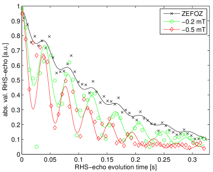
Figure 6: (Color online) Raman-echo decays at ZEFOZ point and with magnetic detunings of -0.2 and -0.5 mT for the z-component.

The decay curves at magnetic fields slightly detuned from the ZEFOZ point show slow modulations with a frequency of $\nu_{M}=24.5\pm 1.7$ Hz. This could be due to a superhyperfine interaction with La nuclei, but a clear explanation is lacking at the present time. This point will be investigated in further experiments. To fit decay times we used the function

$$f(t)=\left(A+M\cos\left(2\pi\nu_{M}t\right)\right)\exp\left({\frac{-t}{T_{2}}}\right)+c,$$

where $A$ is the exponentially decaying part, $\nu_{M}$ is the modulation frequency, $T_{2}$ the decay time and $c$ an offset. As we moved the magnetic field away from the ZEFOZ point $\vec{B}_{opt}$ by $-0.2$ mT in the z-component this resulted in a decrease of the coherence time to $T_{2}(-0.2\mbox{ mT})=133\pm 16$ ms and a shift by $-0.5$ mT resulted in $T_{2}(-0.5\mbox{ mT})=97\pm 19$ ms.

In the following we will use this measured $T_{2}(\vec{B})$ values to estimate the magnetic field fluctuation $\Delta B$ at the Pr³⁺ site. These fluctuations cause frequency shifts and thereby broaden the hyperfine transition. For this purpose, we expand the hyperfine transition frequency $\nu_{i}$ on a deviation $B_{off}$ from a given field $\vec{B}$

$$\nu_{i}\left|{}_{\vec{B}}\right.=\nu_{i}(\vec{B})+s1\,B_{off}+\frac{s2}{2}\,B_{off}^{2}.$$

If the reference field $\vec{B}$ fulfills the ZEFOZ condition, the first derivative vanishes, $s_{1}=0$ and the frequency shift due to the fluctuations is

$$\Delta\nu=\frac{s2}{2}(\Delta B)^{2}.$$ (22)

Since the fluctuations only generate positive frequency shifts (for $s2>0$), they add a line broadening of $\Delta\nu/2$. Using the assumption that the line broadening is entirely due to magnetic field fluctuationsLongdell et al. (2006), we obtain a decay rate

$$T_{2}^{-1}=\frac{s2}{4}(\Delta B)^{2}.$$

With the experimentally obtained value of $T_{2}=158$ ms and $s2\approx 12$ kHz/mT², calculated from the maximum eigenvalue of the derivative matrix Eq. (21), using the parameters from Table 1, we thus estimate the magnetic field fluctuations as $\Delta B\approx 46$ $\mu$T. This value is of the same order of magnitude as that found for the ZEFOZ points in Pr³⁺:Y₂SiO₅, the only ones experimentally investigated up to date, where $s2\approx 3$-$6$ kHz/mT² and $\Delta B=14$ $\mu$T Fraval et al. (2005); Longdell et al. (2006) were found. The zero field relaxation times in Pr³⁺:La₂(WO₄)₃ and Pr³⁺:Y₂SiO₅ are also comparable ($\approx 250$ $\mu$s vs. $\approx 500$ $\mu$s).

We now analyze the dependence of the relaxation times on the magnetic field when the deviation is large compared to the amplitude of the fluctuations, $B_{off}\gg\Delta B$. This changes Eq. (22) to

$$\Delta\nu=\frac{s2}{2}(B_{off}^{2}+2\Delta B\,B_{off}).$$

The first term describes the line shift, the second a line broadening. Using the value $\Delta B\approx 46$ $\mu$T for the magnetic field fluctuations, we expect that the resulting line broadening for a field change of $B_{off}=0.2$ mT is $\approx 9$ ms and for $B_{off}=0.5$ mT $\approx 3.6$ ms. These values are significantly shorter than the experimental values.

The most likely explanation for this discrepancy is that the relaxation at our reference field is not entirely due to magnetic field fluctuations and that the reference field does not exactly fulfill the ZEFOZ condition. Both effects lead to additional contributions to the dephasing rate. We therefore write the total dephasing rate as

$$T_{2}^{-1}=T_{2,0}^{-1}+s1\,\Delta B+s2\,\Delta B\,B_{off}.$$ (23)

Here, $T_{2,0}^{-1}$ describes those contributions that are not due to magnetic field fluctuations, such as phonons, while $s1$ is the first derivative of the transition frequency with respect to the magnetic field change. Both contributions to the dephasing rate are independent of the magnetic field offset $B_{off}$ and therefore not distinguishable in the available experimental data.

Using now $s2\approx 8.2$ kHz/mT², corresponding to the projection of Eq. (21) into the the $z$-direction, we use Eq. (23) to estimate the magnetic field fluctuations. The result of a linear fit of $T_{2}^{-1}$ vs. $B_{off}$ yields $\Delta B\approx 1$ $\mu$T. Applying the same analysis to the Pr³⁺:Y₂SiO₅ data (estimated from Figure 2 in Ref. Fraval et al., 2005) gives $\Delta B\approx 1.3$ $\mu$T. This also reduces the estimate for $\Delta B$ by approximately one order of magnitude compared to the analysis where the minimum dephasing rate is assumed to originate entirely from the quadratic term of the magnetic field fluctuations Longdell et al. (2006).

To get a better estimate for $\Delta B$ further measurements would be required. The phononic contributions to $T_{2}$ could be determined from measurements at different temperatures, as $s1$ and $s2$ are independent of this parameter. Quantitative measurements of $T_{2}$ at several deviations $B_{off}$ in three directions could help to estimate the numerical value of the second term of Eq. (23).

VI Conclusion

We characterized the hyperfine interaction of praseodymium doped into La₂(WO₄)₃ for the electronic ground state and one electronically excited state. We described in detail the experimental and numerical methods to reliably derive the spin Hamiltonian parameters. The relative oscillator strengths between the ³H₄ and ¹D₂ hyperfine levels derived from our data are in good agreement with those measured in earlier experimental work Guillot-Noël et al. (2009). We indicated physical reasons for the experimentally found tensor orientations and their principal axis values by a crystal field analysis discussion. Further the calculated tensor values following from this analysis are in reasonable agreement with the values derived from the experimental data, backing up our results and showing the usefulness of such analysis techniques. The full characterization enabled us to calculate all transition frequencies for arbitrary magnetic fields. Using this, we could predict the magnetic field value at which a ZEFOZ transition occurs. We verified this condition experimentally in a second laboratory. Besides the experimental verification of the hyperfine characterization, we determined the order of magnitude of the magnetic fluctuations at the Pr³⁺-site ($\Delta B\lesssim 10$ $\mu$T) and investigated the coherence properties of the ZEFOZ transition. The latter showed characteristics similar to superhyperfine interaction and a up to 630-fold increase of the coherence lifetime compared to zero field. The demonstrated spin lifetime of 158 $\pm$ 7 ms and the relatively low second order Zeeman coefficient show that even crystal systems with high magnetic moment density can have a high potential for quantum memory and information applications.

Appendix A Euler angles conventions

For the tensor transformations we used the common “zyz”-convention Goldstein et al. (2002) with right-handed coordinate systems. The transformation matrices $R$, e.g. in Eq. 8 and 12, are given by:

$$A=\left(\begin{array}[]{ccc}\cos\alpha&\sin\alpha&0\\ -\sin\alpha&\cos\alpha&0\\ 0&&1\end{array}\right),B=\left(\begin{array}[]{ccc}\cos\beta&0&-\sin\beta\\ 0&1&0\\ \sin\beta&0&\cos\beta\end{array}\right),C=\left(\begin{array}[]{ccc}\cos\gamma&\sin\gamma&0\\ -\sin\gamma&\cos\gamma&0\\ 0&&1\end{array}\right)$$

$$R\left(\alpha,\beta,\gamma\right)=C\cdot B\cdot A=\left(\begin{array}[]{ccc}-\sin\alpha\sin\gamma+\cos\alpha\cos\beta\cos\gamma&\cos\alpha\sin\gamma+\cos\beta\cos\gamma\sin\alpha&-\cos\gamma\sin\beta\\ -\cos\gamma\sin\alpha-\cos\alpha\cos\beta\sin\gamma&\cos\alpha\cos\gamma-\cos\beta\sin\alpha\sin\gamma&\sin\beta\sin\gamma\\ \cos\alpha\sin\beta&\sin\alpha\sin\beta&\cos\beta\end{array}\right),$$ (24)

with $\alpha$, $\gamma$ $\epsilon$ $[-\pi,\pi]$ and $\beta$ $\epsilon$ $[0,\pi]$.

References

- Longdell et al. (2004) J. J. Longdell, M. J. Sellars, and N. B. Manson, Phys. Rev. Lett., 93, 130503 (2004).
- Rippe et al. (2008) L. Rippe, B. Julsgaard, A. Walther, Y. Ying, and S. Kröll, Phys Rev A, 77, 022307 (2008).
- Wesenberg et al. (2007) J. H. Wesenberg, K. Mølmer, L. Rippe, and S. Kröll, Phys Rev A, 75, 012304 (2007).
- Nilsson and Kröll (2005) M. Nilsson and S. Kröll, Optics Communications, 247, 393 (2005).
- Afzelius et al. (2009) M. Afzelius, C. Simon, H. deRiedmatten, and N. Gisin, Phys Rev A, 79, 52329 (2009).
- Hétet et al. (2008) G. Hétet, J. J. Longdell, A. L. Alexander, P. K. Lam, and M. J. Sellars, Phys. Rev. Lett., 100, 023601 (2008).
- Lauro et al. (2009) R. Lauro, T. Chanelière, and J.-L. LeGouët, Phys Rev A, 79, 53801 (2009).
- Hedges et al. (2010) M. P. Hedges, J. J. Longdell, Y. Li, and M. J. Sellars, Nature, 465, 1052 (2010).
- Usmani et al. (2010) I. Usmani, M. Afzelius, H. de Riedmatten, and N. Gisin, Nature Communications, 1, 1 (2010).
- Bonarota et al. (2011) M. Bonarota, J.-L. Le Gouët, and T. Chanelière, New. J. Phys., 13, 013013 (2011).
- Clausen et al. (2011) C. Clausen, I. Usmani, F. Bussieres, N. Sangouard, M. Afzelius, H. de Riedmatten, and N. Gisin, Nature, 469, 508 (2011), ISSN 0028-0836.
- Saglamyurek et al. (2011) E. Saglamyurek, N. Sinclair, J. Jin, J. A. Slater, D. Oblak, F. Bussieres, M. George, R. Ricken, W. Sohler, and W. Tittel, Nature, 469, 512 (2011), ISSN 0028-0836.
- Böttger et al. (2009) T. Böttger, C. W. Thiel, R. L. Cone, and Y. Sun, Phys. Rev. B, 79, 115104 (2009).
- Fraval et al. (2005) E. Fraval, M. J. Sellars, and J. J. Longdell, Phys. Rev. Lett., 95, 030506 (2005).
- Fraval et al. (2004) E. Fraval, M. J. Sellars, and J. J. Longdell, Phys. Rev. Lett., 92, 077601 (2004).
- Longdell et al. (2006) J. J. Longdell, A. L. Alexander, and M. J. Sellars, Phys. Rev. B, 74, 195101 (2006).
- Tittel et al. (2010) W. Tittel, M. Afzelius, T. Chaneliére, R. L. Cone, S. Kröll, S. A. Moiseev, and M. Sellars, Laser & Photon. Rev., 4, 244 (2010).
- Shannon and Prewitt (1969) R. D. Shannon and C. T. Prewitt, Acta Crystallographica Section B: Structural Crystallography and Crystal Chemistry, 25, 925 (1969).
- Guillot-Noël et al. (2009) O. Guillot-Noël, P. Goldner, F. Beaudoux, Y. LeDu, J. Lejay, A. Amari, A. Walther, L. Rippe, and S. Kröll, Phys. Rev. B, 79, 155119 (2009).
- Goldner et al. (2009) P. Goldner, O. Guillot-Noël, F. Beaudoux, Y. LeDu, J. Lejay, T. Chanelière, J. L. LeGouët, L. Rippe, A. Amari, A. Walther, and S. Kröll, Phys Rev A, 79, 33809 (2009).
- Longdell et al. (2002) J. J. Longdell, M. J. Sellars, and N. B. Manson, Phys. Rev. B, 66, 35101 (2002).
- Macfarlane and Shelby (1987) R. M. Macfarlane and R. M. Shelby, in Spectroscopy of Solids Containing Rare Earth Ions, Modern Problems in Condensed Matter Sciences, Vol. 21, edited by A. A. Kaplyanskii and R. M. Macfarlane (North Holland, 1987) pp. 51–184.
- Teplov (1968) M. A. Teplov, Soviet Physics JETP, 26, 872 (1968).
- Baker and Bleaney (1958) J. M. Baker and B. Bleaney, Proceedings of the Royal Society of London. Series A, 245, 156 (1958).
- Guillot-Noël et al. (2007) O. Guillot-Noël, P. Goldner, Y. LeDu, P. Loiseau, B. Julsgaard, L. Rippe, and S. Kröll, Phys. Rev. B, 75, 205110 (2007).
- Mlynek et al. (1983) J. Mlynek, N. C. Wong, R. G. DeVoe, E. S. Kintzer, and R. G. Brewer, Phys. Rev. Lett., 50, 993 (1983).
- Wong et al. (1983) N. C. Wong, E. S. Kintzer, J. Mlynek, R. G. Devoe, and R. G. Brewer, Physical Review B (Condensed Matter), 28, 4993 (1983).
- Mitsunaga et al. (1984) M. Mitsunaga, E. S. Kintzer, and R. G. Brewer, Phys. Rev. Lett., 52, 1484 (1984).
- Mitsunaga et al. (1985) M. Mitsunaga, E. S. Kintzer, and R. G. Brewer, Physical Review B (Condensed Matter), 31, 6947 (1985).
- Kirkpatrick et al. (1983) S. Kirkpatrick, C. D. Gelatt, and M. P. Vecchi, Science, 220, 671 (1983).
- Audet and Dennis (2003) C. Audet and J. E. Dennis, Siam J Optimiz, 13, 889 (2003).
- Note (1) The negative sign of the gyromagnetic ratios preserves the consistence with the crystal field analysis in Sec. V.3. It should be noted that this analysis assumes a higher crystal symmetry than the actual one of Pr3+:La2(WO4)3 and that RHS spectra are not sensitive to the sign of the gyromagnetic ratios, as explained later.
- Goldstein et al. (2002) H. Goldstein, C. P. Poole, and J. L. Safko, Classical mechanics (Addison Wesley, 2002) p. 638.
- Longdell (2003) J. J. Longdell, Quantum information processing in rare earth ion doped insulators, Ph.D. thesis, Australian National University (2003).
- Guillot-Noël et al. (2010) O. Guillot-Noël, Y. LeDu, F. Beaudoux, E. Antic-Fidancev, M. F. Reid, R. Marino, J. Lejay, A. Ferrier, and P. Goldner, Journal of Luminescence, 130, 1557 (2010).
- Abragam (1994) A. Abragam, The Principles of Nuclear Magnetism (Oxford University Press, 1994) p. 599.
- Note (2) These parameters differ from those of Ref. \rev@citealpnumGuillotNoel:2010p1250 which correspond to another assignement of crystal field axes.
- Esterowitz et al. (1979) L. Esterowitz, F. J. Bartoli, R. E. Allen, D. E. Wortman, C. A. Morrison, and R. P. Leavitt, Physical Review B (Condensed Matter), 19, 6442 (1979).
- Nilsson et al. (2004) M. Nilsson, L. Rippe, S. Kröll, R. Klieber, and D. Suter, Phys. Rev. B, 70, 214116 (2004).
- Nilsson et al. (2005) M. Nilsson, L. Rippe, S. Kröll, R. Klieber, and D. Suter, Phys. Rev. B, 71, 149902(E) (2005).