Probing deconfinement in a chiral effective model with Polyakov loop at imaginary chemical potential

Abstract

The phase structure of the two-flavor Polyakov-loop extended Nambu-Jona-Lashinio model is explored at finite temperature and imaginary chemical potential with a particular emphasis on the confinement-deconfinement transition. We point out that the confined phase is characterized by a $\cos 3\mu_{I}/T$ dependence of the chiral condensate on the imaginary chemical potential while in the deconfined phase this dependence is given by $\cos\mu_{I}/T$ and accompanied by a cusp structure induced by the $Z(3)$ transition. We demonstrate that the phase structure of the model strongly depends on the choice of the Polyakov loop potential $\mathcal{U}$. Furthermore, we find that by changing the four fermion coupling constant $G_{s}$, the location of the critical endpoint of the deconfinement transition can be moved into the real chemical potential region. We propose a new parameter characterizing the confinement-deconfinement transition.

I Introduction

The exploration of the phase diagram of strongly interacting matter has received a lot of attention in recent years. First principle calculations of the phase structure from the Lagrangian of Quantum Chromodynamics (QCD) is intrinsically difficult owing to the strongly coupled nature of the theory at large distances. Lattice Gause Theory (LGT) calculations provide a unique and powerful tool for studying QCD in the non-perturbative regime. Increasing computer power has recently made LGT simulations at almost physical quark masses possible Bazavov et al. (2009); Aoki et al. (2009). The results indicate that the transition from the confined, chirally broken phase to the deconfined, chirally restored phase at $T\sim 160$ MeV  and vanishing baryon chemical potential, $\mu_{B}=0$, is of the crossover type fodor .

For non-zero net baryon density, LGT calculations suffer from the so-called “sign problem”. For finite quark chemical potential (and $N_{c}=3$), the statistical weight of the Monte-Carlo simulation becomes non positive definite due to the complex fermion determinant. This issue has impeded the progress in LGT calculations at finite densities.

There have been several attempts to bypass the sign problem Muroya et al. (2003). One interesting approach involves using an imaginary chemical potential, for which the fermion determinant is real and, therefore, systematic LGT simulations are possible Roberge and Weiss (1986). There are two major ways for extracting information on the real phase diagram from calculations at imaginary chemical potential. One is to project the grand partition function $Z_{G}$ computed at imaginary chemical potential onto the canonical partition function

$$Z_{c}(T,V,N_{q})=\intop_{0}^{2\pi}\frac{d(\beta\mu_{I})}{2\pi}e^{-i\beta\mu_{I}N_{q}}Z_{G}(T,V,\mu_{q}=i\mu_{I}).$$ (1)

In spite of the difficulties involved in the evaluation of the oscillatory integral, there are lattice calculations aimed at studying the phase diagram in the temperature-number density plane by means of this approach Ejiri (2008); Li et al. (2010). An alternative way involves an analytic continuation from imaginary to real values of the chemical potential. This method has proven quite powerful for determining the critical line at $\mu_{q}<\pi T/3$ de Forcrand and Philipsen (2002) and this approach has been applied in LGT calculations de Forcrand and Philipsen (2003); D’Elia and Lombardo (2003); Papa ; D’Elia and Lombardo (2004); Chen and Luo (2005); D’Elia et al. (2007); de Forcrand and Philipsen (2007); Wu et al. (2007); de Forcrand and Philipsen (2010); Nagata and Nakamura (2011), in resummed perturbation theory Hart et al. (2001), as well as in quasiparticle models Bluhm and Kämpfer (2008). Of course, the analytic continuation requires knowledge of the analytic structure of the thermodynamic functions. Therefore effective models that share the symmetries of QCD are useful for testing such approaches, because a result obtained by analytic continuation from imaginary chemical potential can be confronted with the known solution at real chemical potential.

A remarkable feature of QCD at imaginary chemical potential is the Roberge-Weiss (RW) transition at $\mu_{q}/T=\pi/3+2\pi k/3$, where $k$ is an integer Roberge and Weiss (1986). The RW transition involves a shift from one $Z(3)$ sector to another in the deconfined phase. This transition is a remnant of the $Z(3)$ symmetry of the pure gauge theory, which is explicitly broken in the presence of fermions of finite mass. Note that in this case the Polyakov loop is not an exact order parameter. Using perturbation theory Roberge and Weiss (1986), Roberge and Weiss showed that this phase transition is first-order. This was confirmed in subsequent lattice simulations de Forcrand and Philipsen (2002). While it was expected that the RW transition is a signature of the deconfined phase Weiss (1987), the transition line, which is parallel to the temperature axis at $\mu_{I}/T=\pi/3$, terminates at a temperature above the deconfinement transition temperature at vanishing chemical potential. Since the characteristics of the endpoint and its implications for the phase diagram at real $\mu$ are still debated de Forcrand and Philipsen (2010); Wu et al. (2007); Kouno et al. (2009); D’Elia and Sanfilippo (2009); Sakai et al. (2010a); Bonati et al. (2011); Aarts , it is interesting to explore the phase structure at imaginary chemical potential in an effective model. The aim of this paper is to characterize the phase structure especially of the confinement-deconfinement transition of QCD at imaginary chemical potential in the framework of an effective model which exhibits the relevant symmetries.

In this work we use the Polyakov-loop-extended Nambu-Jona-Lasinio (PNJL) model Fukushima (2004); Ratti et al. (2006). The NJL model Nambu and Jona-Lasinio (1961a, b) describes many aspects of QCD related to chiral symmetry Hatsuda and Kunihiro (1994). This model, however, lacks confinement. On the other hand, thermal models with internal gauge symmetry have been studied. These models reveal a RW transition Elze et al. (1987); Miller and Redlich (1988) while chiral symmetry is not realized. The PNJL model is an effective model of QCD, which ameliorates some of the shortcomings of the NJL model by introducing a coupling of the quark field to a uniform background gauge field $A_{0}$. It has been demonstrated that the PNJL model reproduces the RW transition Sakai et al. (2008a). The authors of Ref. Sakai et al. (2008a) have studied the phase structure of the PNJL model in detail (see also Sakai et al. (2008b, c); Kouno et al. (2009); Sakai et al. (2009, 2010b, 2010a); Kashiwa et al. (2011)). These studies indicate that various improvements are necessary in order to reproduce the lattice data. In this paper, applying the simplest interaction term in the PNJL model as introduced in Ref. Sakai et al. (2008a), we focus on differences in the behaviour of the order parameters dependently on the parametrizations of the effective Polyakov loop potential. We characterize the phase structure qualitatively through a systematic comparison of the results for different Polyakov loop potentials and give perspectives on the nature of the phase transitions at imaginary chemical potential.

We introduce a new quantity, which characterizes the confinement-deconfinement transition based on the characteristic dependence of the chiral condensate on the imaginary chemical potential. The relation of this parameter to the so called dual order parameter Bilgici et al. (2008) is discussed.

The paper is organized as follows: in the next section we briefly review the basic properties of the QCD partition function which are relevant for this study. The model is introduced in Sec. III and results of the numerical calculation are presented in Sec. IV. In Sec. V, we discuss the parameters characterizing the confinement-deconfinement transition and finally in Section VI we summarize.

II General properties of the QCD partition function at imaginary chemical potential

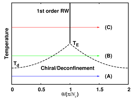
Figure 1: Schematic phase diagram on $T-\theta$ plane. The solid line denotes the first-order Roberge-Weiss transition line which terminates at $T=T_{E}$, while the dashed line shows the transition line of the chiral and confinement-deconfinement transitions. The arrows labeled A–C indicate paths probed in Sec. IV.

The partition function of the $SU(N_{c})$ gauge theory with fermions, is characterized by the number operator $\hat{N}=\int d^{3}x\,q^{\dagger}q$, at imaginary chemical potential $\theta=\mu_{I}/T=\beta\mu_{I}$.

$$Z_{G}(T,V,\theta)=\text{Tr}\left[e^{-\beta H+i\theta\hat{N}}\right].$$ (2)

The partition function can be expressed in terms of the functional integral

$$Z_{G}(T,V.\theta)=\int\mathcal{D}q\mathcal{D}\bar{q}\mathcal{D}A_{\mu}e^{-S_{E}(\beta,\theta)}$$ (3)

where $S_{E}$ is the Euclidean action

$$S_{E}=\int_{0}^{\beta}d\tau\int d^{3}x\,\bar{q}(\gamma\cdot D-m)q-\frac{1}{4}G^{2}-i\frac{\theta}{\beta}q^{\dagger}q.$$ (4)

In (3), the gauge and quark field obey periodic and anti-periodic boundary conditions in the temporal interval $[0,\beta]$, respectively. The particle-antiparticle symmetry implies, that $Z_{G}$ is an even function of $\theta$, $Z_{G}(T,V,-\theta)=Z_{G}(T,V,\theta)$.

By performing the change of variables $q\rightarrow e^{i\theta\tau/\beta}q$, the explicit dependence imaginary chemical potential in the action can be removed and converted into a modified boundary condition Weiss (1987); Roberge and Weiss (1986)

$$q(x,\beta)=-e^{i\theta}q(x,0).$$ (5)

Then $Z(N_{c})$ transformation

$$q\rightarrow Uq,\quad A_{\mu}\rightarrow UA_{\mu}U^{-1}-(i/g)(\partial_{\mu}U)U^{-1}$$ (6)

with $U(x,\beta)=\exp(2\pi ik/N_{c})U(x,0)$ leaves the action and the functional measure invariant, but modifies the boundary condition

$$q(x,\beta)=-e^{i\theta}e^{\frac{2\pi i}{N_{c}}k}q(x,0),$$ (7)

where $k$ is an integer Weiss (1987); Roberge and Weiss (1986). A comparison of Eqs. (7) and (5) reveals that the partition function is periodic with respect to finite shifts of $\theta$

$$Z_{G}(T,V,\theta)=Z_{G}\left(T,V,\theta+\frac{2\pi k}{N_{c}}\right).$$ (8)

This periodicity is a remnant of the $Z(N_{c})$ symmetry, the center symmetry of the $SU(N_{c})$ gauge group. In the presence of fermions the $Z(N_{c})$ symmetry is explicitly broken. In other words, the partition function is invariant under the transformation $\theta\rightarrow\theta+2\pi k/N_{c}$ combined with the $Z(N_{c})$ transformation. This symmetry was dubbed “extended $Z(N_{c})$ symmetry” in Ref. Sakai et al. (2008a). It is easy to see that the thermodynamic potential $\Omega=-T\ln Z_{G}$ and the chiral condensate $\sigma\equiv\langle\bar{q}q\rangle=-\frac{1}{V}\frac{\partial\Omega}{\partial m_{0}}$, with $m_{0}$ being the current quark mass, have the same periodicity.

Roberge and Weiss noted the existence of the first-order transition at $\theta=\pi/N_{c}+2\pi k/N_{c}$ in the deconfined phase  Roberge and Weiss (1986). It was expected that the RW transition takes place at the same temperature as the confinement-deconfinement transition temperature $T_{d}$. Lattice simulations, however, showed that the endpoint of the RW transition is at a temperature $T_{E}$, which is higher than $T_{d}$. A schematic phase diagram for imaginary chemical potantial is shown in Fig. 1. The nature of the chiral and confinement-deconfinement transition at finite $\theta$ is not fully understood yet. First, there is no a priori reason that these two transitions coincide. LGT simulations, however, show that the two transitions take place at approximately the same temperature de Forcrand and Philipsen (2002); D’Elia and Lombardo (2003); Wu et al. (2007). Second, the order of the transition depends on the quark mass and the number of flavors. For $N_{f}=2$ and $N_{c}=3$ (this case will be explored in this paper) Ref. Wu et al. (2007) shows that for $m_{\pi}/m_{\rho}\simeq 0.9$ the chiral and confinement-deconfinement transition at $\theta=0.92(\pi/3)$ is of the crossover type, implying that the transition at the RW endpoint is second order. On the other hand, Refs. D’Elia and Sanfilippo (2009); de Forcrand and Philipsen (2010) have demonstrated that for light and heavy quark masses, the phase transition at $T_{E}$ is first-order. In this case, the first-order RW line continues along the dashed lines and terminates at a critical endpoint which is located at a value of the imaginary chemical potential $0<\theta<\pi/N_{c}$.

In this paper, we do not attempt to obtain a fit of the PNJL model to lattice results at imaginary chemical potential. Rather, we focus on exploring qualitative features of the phase structure of the model and their origin.

III PNJL model

III.1 Formulation

Studies of the phase diagram of strongly at imaginary chemical potential within effective models, requires a model with the same symmetry structure as QCD. The most important symmetries which must be accounted for are the extended $Z(3)$ and the chiral symmetries. In this article we employ the Polyakov loop extended Nambu-Jona-Lasinio (PNJL) model with $N_{f}=2$ and $N_{c}=3$ Fukushima (2004); Ratti et al. (2006), which respects the above mentioned symmetries.

The Lagrangian of the two-flavor PNJL model with a four-quark interaction is given by

$$\mathcal{L}=\bar{q}(i\gamma_{\mu}D^{\mu}-m_{0})q+G_{s}[(\bar{q}q)^{2}+(\bar{q}i\gamma_{5}\vec{\tau}q)^{2}]$$

$$-\mathcal{U}(\Phi[A],\Phi^{*}[A];T).$$ (9)

In the covariant derivative $D^{\mu}=\partial^{\mu}-iA^{\mu}$, only the temporal component $A_{0}$ of the gluon field $A_{\mu}=gA_{\mu}^{a}\lambda^{a}/2$ is included. The gluon field is treated as a classical background field, whose dynamics is encoded in the effective potential $\mathcal{U}$. The gluon field is expressed in terms of the traced Polyakov loop and its conjugate

$$\Phi=\frac{1}{3}\langle\text{Tr}_{c}L\rangle,\quad\Phi^{*}=\frac{1}{3}\langle\text{Tr}_{c}L^{\dagger}\rangle;$$ (10)

where the trace is taken over color space and

$$L(\boldsymbol{x})=\mathcal{P}\exp\left[i\int_{0}^{\beta}d\tau A_{4}(\boldsymbol{x},\tau)\right].$$ (11)

Here $A_{4}=iA_{0}$ and and $\mathcal{P}$ denotes the path ordering in Euclidean time $\tau$. In the Polyakov gauge the matrix $L$ reduces to the diagonal form $L=\text{diag}(e^{i\phi_{1}},e^{i\phi_{2}},e^{-i(\phi_{1}+\phi_{2})})$ Fukushima (2004). Note that in general $\Phi^{*}$ is not the complex conjugate of $\Phi$. At real chemical potential both $\Phi$ and $\Phi^{*}$ are real and at $\mu\neq 0$ their values differ Sasaki et al. (2007). At imaginary chemical potential, $\Phi^{*}$ is the complex conjugate of $\Phi$ and they have non-zero imaginary parts Sakai et al. (2008a). Therefore, in the discussion below, we use the notation

$$\Phi =|\Phi|e^{i\phi},$$ (12)

$$\Phi^{*} =|\Phi|e^{-i\phi}$$ (13)

for imaginary $\mu$. The extended $Z(3)$ symmetry leads to the following properties of the Polyakov loop Sakai et al. (2008a)

$$\left|\Phi\left(\theta+\frac{2\pi k}{3}\right)\right| =|\Phi(\theta)|,$$ (14)

$$|\Phi(-\theta)| =|\Phi(\theta)|,$$ (15)

$$\phi\left(\theta+\frac{2\pi k}{3}\right) =\phi(\theta)-\frac{2\pi k}{3},$$ (16)

$$\phi(-\theta) =-\phi(\theta).$$ (17)

In the mean-field approximation the thermodynamic potential can be written in terms of quark quasiparticles with a dynamical mass $M$, momentum $p=|\boldsymbol{p}|$, and energy $E_{p}=\sqrt{p^{2}+M^{2}}$ Fukushima (2004); Sakai et al. (2008a)

$$\Omega(T,V,\theta) =-4V\int\frac{d^{3}p}{(2\pi)^{3}}\left[3(E_{p}-E_{p}^{0})\right.$$

$$\left.+\frac{1}{\beta}\ln[1+3(\Phi+\Phi^{*}e^{-\beta E^{-}_{p}})e^{-\beta E^{-}_{p}}+e^{-3\beta E^{-}_{p}}]\right.$$

$$\left.+\frac{1}{\beta}\ln[1+3(\Phi^{*}+\Phi e^{-\beta E^{+}_{p}})e^{-\beta E^{+}_{p}}+e^{-3\beta E^{+}_{p}}]\right]$$

$$+(G_{s}\sigma^{2}+\mathcal{U})V.$$ (18)

The term in the first line represents the ultraviolet divergent vacuum fluctuations. As usual, we introduce a three-momentum cutoff $\Lambda$ in the momentum integration to regularize the vacuum contribution. We subtract the vacuum term with the single-quark energy $E_{p}^{0}=\sqrt{p^{2}+m_{0}^{2}}$, so that the vacuum contribution vanishes when the chiral symmetry is restored, as in Ref. Sasaki et al. (2007). We use a short-hand notation, where the imaginary chemical potential is subsumed in $E^{\pm}_{p}=E_{p}\pm i\theta/\beta$. The dynamical mass $M$ is related to the current quark mass and the chiral condensate $\sigma=\langle\bar{q}q\rangle$ by $M=m_{0}-2G_{s}\sigma$. The term $G_{s}\sigma^{2}$ in the last line is due to the meson potential in the Lagrangian (9).

Table 1: Parameters in the polynomial potential (19).

$T_{0}$[MeV]	$a_{0}$	$a_{1}$	$a_{2}$	$a_{3}$	$b_{3}$	$b_{4}$
$270$	$6.75$	$-1.95$	$2.625$	$-7.44$	$0.75$	$7.5$

Table 2: Parameters in the logarithmic potential (21).

$T_{0}$[MeV]	$a_{0}$	$a_{1}$	$a_{2}$	$b_{3}$
270	3.51	$-2.47$	$15.22$	$-1.75$

So far two types of the Polyakov loop effective potential $\mathcal{U}$ have been widely used. The polynomial potental has as a general $Z(3)$ symmetric form Pisarski (2000); Ratti et al. (2006):

$$\frac{\mathcal{U}_{\text{poly}}}{T^{4}}=-\frac{b_{2}(T)}{2}\Phi^{*}\Phi-\frac{b_{3}}{6}\left[\Phi^{3}+(\Phi^{*})^{3}\right]+\frac{b_{4}}{4}(\Phi^{*}\Phi)^{2}$$ (19)

with

$$b_{2}(T)=a_{0}+a_{1}\frac{T_{0}}{T}+a_{2}\left(\frac{T_{0}}{T}\right)^{2}+a_{3}\left(\frac{T_{0}}{T}\right)^{3}.$$ (20)

The coefficients are determined by fitting the equation of state and the expectation value of the Polyakov loop to lattice data of pure gauge theory Boyd et al. (1996); Kaczmarek et al. (2002) in Ref. Ratti et al. (2006). In the other widely used variant, a logarithmic potential motivated by the strong coupling expansion is implemented Fukushima (2004); Roessner et al. (2007)

$$\frac{\mathcal{U}_{\text{log}}}{T^{4}}= -\frac{a(T)}{2}\Phi^{*}\Phi+b(T)$$

$$\times\log\left\{1-6\Phi^{*}\Phi+4\left[\Phi^{3}+(\Phi^{*})^{3}\right]-3(\Phi^{*}\Phi)^{2}\right\}$$ (21)

where

$$a(T)=a_{0}+a_{1}\frac{T_{0}}{T}+a_{2}\left(\frac{T_{0}}{T}\right)^{2},\quad b(T)=b_{3}\left(\frac{T_{0}}{T}\right)^{3}.$$ (22)

The above parameterization for the temperature dependency was introduced in Roessner et al. (2007) and the constants are determined by fitting lattice data of pure SU(3) theory. In Ref. Fukushima (2004), a similar functional form in $\Phi$ but different parameterization of the temperature dependence was introduced. In this potential, however, one of the parameters is fixed to reproduce the simultaneous crossover transition for chiral and deconfinement transition rather than the pure gauge theory except for the transition temperature $T_{0}\simeq 270$ MeV. We refer to Fukushima2008 for discussion. This difference makes it difficult to perform a systematic comparison of effect of quarks near the deconfinement transition. If we re-fit the parameters to reproduce the pure SU(3) lattice data, we expect to have similar results to those from the logarithmic potential (21) since the target space and the transition temperature are the same. In this paper, we focus on the two potentials Eqs. (19) and (21) which equally reproduce the Polyakov loop and thermodynamics as well as the first order confinement-deconfinement phase transition. We use the parameters determined in Refs. Ratti et al. (2006) and Roessner et al. (2007). For convenience, they are summarized in Tables 2 and 2.

The order parameters, chiral condensate $\sigma$ (or dynamical mass $M$), modulus of the Polyakov loop $|\Phi|$, and the phase of the Polyakov loop $\phi$ are determined numerically by solving the coupled equations of motion

$$\frac{\partial\Omega(T,V,\theta;M,|\Phi|,\phi)}{\partial X_{i}}=0,\quad X_{i}=M,|\Phi|,\phi.$$ (23)

The phase diagram in the $T-\theta$ plane of the polynomial potential model (19) has been studied in Refs. Sakai et al. (2008a, b). In this model, the first-order Roberge-Weiss transition at $\theta=\pi/3\pm 2\pi k/3$, the second-order chiral transition in the chiral limit and the crossover one at finite quark mass as well as the crossover confinement-deconfinement transition were found. However, these features, depend on the choice of the Polyakov loop effective potential and further quark interaction terms are required to reproduce lattice results quantitatively Sakai et al. (2010a, 2008b).

In this paper, we restrict ourselves to the simplest quark-quark interaction form, as shown in Eq. (9) and focus on behavior of the order parameters in the $T-\theta$ plane for the polynomial and logarithmic Polyakov loop potentials.

III.2 Some analytic insights

Before proceeding to the full numerical computation, it is useful to explore the general properties of the thermodynamic potential (III.1) analytically in a few limiting cases. The momentum integration in Eq. (III.1) can be carried out analytically if we first expand the logarithmic terms in the integrand in powers of $e^{-\beta E_{p}}\ll 1$. We thus find, keeping terms up to order $(e^{-\beta E_{p}})^{3}$,

$$\Omega\simeq (G_{s}\sigma^{2}+\mathcal{U})V-\Omega_{0}-\frac{2V}{\beta\pi^{2}}$$

$$\times \left[3(\Phi e^{i\theta}+\Phi^{*}e^{-i\theta})\intop_{0}^{\Lambda}dpp^{2}e^{-\beta E_{p}}\right.$$

$$+ \frac{3}{2}\left\{e^{2i\theta}(2\Phi^{*}-3\Phi^{2})+e^{-2i\theta}(2\Phi-3\Phi^{*2})\right\}\intop_{0}^{\Lambda}dpp^{2}e^{-2\beta E_{p}}$$

$$+ \left\{2(1-9\Phi\Phi^{*})\cos 3\theta+9e^{3i\theta}\Phi^{3}+9e^{-3i\theta}\Phi^{*3}\right\}$$

$$\times \left.\intop_{0}^{\Lambda}dpp^{2}e^{-3\beta E_{p}}\right].$$ (24)

Here, $\Omega_{0}$ is the temperature independent vacuum term. While it is necessary to introduce a finite cutoff for this term, due to the non-renormalizability of the PNJL model, taking $\Lambda\rightarrow\infty$ in the thermal part does not affect the qualitative features discussed below. Thus the momentum integration of the thermal part can be carried explcitily resulting in modified Bessel functions $K_{n}$.

We first consider the low temperature limit $\Phi=\Phi^{*}=0$ in order to explore the effect of the Polyakov loop in the confined phase. In this case the Polyakov loop effective potential, $\mathcal{U}$, vanishes. Furthermore, the gap equation for the dynamical mass $M$, obtained from Eq. (24), $\partial\Omega/\partial M=0$, reduces to

$$M\simeq m_{0} +\frac{6G_{s}}{\pi^{2}}[M^{3}f(\Lambda/M)-m_{0}^{3}f(\Lambda/m_{0})]$$

$$-\frac{8G_{s}M^{2}T\cos 3\theta}{\pi^{2}}K_{1}(3M/T),$$ (25)

where

$$f(x)=x\sqrt{x^{2}+1}-\ln(x+\sqrt{x^{2}+1}).$$ (26)

Note that, for $3M/T\gg 1$,

$$K_{1}(3M/T)\sim\sqrt{\frac{\pi T}{6M}}e^{-3M/T}.$$ (27)

The gap equation (25) implies that the $\theta$ dependence of the dynamical mass is completely determined by $\cos 3\theta$ term. Consequently, $M$ is a periodic function of $\theta$ with the period $2\pi/3$, as expected. For small temperatures, quark degrees of freedom are strongly suppressed, $\sim e^{-3M/T}$, since, for a vanishing Polyakov loop, only three-quark clusters survive. The chiral phase transition takes place when the thermal contribution in the gap equation is of the same order as the vacuum term. If the condition $\Phi=\Phi^{*}=0$ is strictly enforced, the chiral transition is shifted to very high temperatures. Because the thermal excitation of quarks in this limit is possible only in three quark clusters, the resulting thermodynamics is qualitatively similar to that of the nucleonic NJL model, which also yields a very high chiral transition temperature Sasaki and Mishustin (2010).

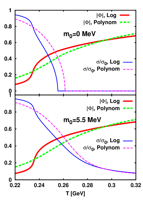
Figure 2: Temperature dependence of the chiral condensate normalized by the value at $T=0$ and the Polyakov loop at vanishing chemical potential. Upper panel shows the result in the chiral limit while the lower stands for the physical quark mass.

In the (naive) high-temperature limit, $\Phi=\Phi^{*}\to 1$, the gap equation reduces to that of the ordinary NJL model,

$$M=m_{0} +\frac{6G_{s}}{\pi^{2}}[M^{3}f(\Lambda/M)-m_{0}^{3}f(\Lambda/m_{0})]$$

$$-\frac{24G_{s}M^{2}T\cos\theta}{\pi^{2}}K_{1}(M/T).$$ (28)

Now, the $\theta$ dependence of the dynamical mass is determined by $\cos\theta$ and the thermal factor is proportional to $K_{1}(M/T)$, appropriate for the thermal excitation of single quarks. In this case, the dynamical mass has lost the original periodicity of the partition function (8), which is respected in the low-temperature limit (25).

At $\theta=\pi/2$ the thermal contribution in (28) vanishes and consequently the dynamical mass equals its vacuum value, irrespective of temperature. Hence, in this approximation the phase boundary is shifted to higher temperatures as the imaginary chemical potential is increased, and eventually approaches $T=\infty$ in the limit $\theta\to\pi/2$. In general, the thermal contribution is of the form $-\sum_{n}L_{n}\cos n\theta K_{1}(nM/T)$ with $L_{n}>0$. Due to the higher order terms, the transition temperature remains finite, but the positive curvature of the phase boundary persists . On the other hand, for real chemical potentials the leading thermal contribution is proportional to $T\cosh\beta\mu$. Since $\cosh x$ is an increasing function of $x$, this implies that the chiral transition temperature decreases as the real chemical potential grows.

In the high-temperature limit, as implemented above, the original periodicity of the partition function is lost because the phase of the Polyakov loop is neglected. In fact, at imaginary chemical potential, the high temperature limit of the PNJL model is in general not the NJL model. The Roberge-Weiss transition, characterized by discontinuous jumps of the phase $\phi$, preserves the periodicity $2\pi/3$ in the deconfinement phase.

IV Behavior of the order parameters at imaginary chemical potential

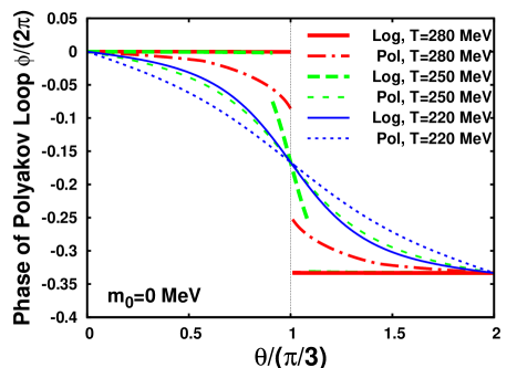
Figure 3: Phase of Polyakov loop as a function of $\theta$ for various temperatures in the chiral limit. As in Fig. 2, each line stands for the results of the logarithmic Polyakov loop potential and the polynomial one at the different temperatures, respectively.

We now discuss the characteristics of the order parameters obtained by solving the full gap equation Eq. (23). Besides the Polyakov loop potentials, given in the previous section, the model has three parameters in the fermion sector. We use

$$G_{s} =5.498\text{GeV}^{-2},$$ (29)

$$\Lambda =0.6315\text{GeV},$$ (30)

which reproduce the vacuum pion mass and pion decay constant at zero temperature and density, when the current quark mass is fixed to the value $m_{0}=5.5$ MeV  Hatsuda and Kunihiro (1994).

In what follows, we compare the results obtained for a finite pion mass with those corresponding to the chiral limit, $m_{0}=0$. In the latter case, the model belongs to the universality class of the three dimensional $O(4)$ spin model and exhibits a second-order phase transition at finite temperature and small values of the real chemical potential.

With the parameter set given above, we find the chiral condensate and the Polyakov loop shown in Fig. 2. The dependence of the order parameters on the temperature shows that in the chiral limit, the chiral transition is indeed second-order, while the confinement-deconfinement transition is of the cross over type. For finite quark mass, $m_{0}=5.5$ MeV, shown in the lower panel, the chiral order parameter and the Polyakov loop both exhibit smooth crossover transitions. Thus, the explicit symmetry breaking induces a qualitative change of the chiral condensate, while for the Polyakov loop this dependence is negligible. Furthermore, a comparison of the two parametrizations of the Polyakov loop effective potential shows that the transition is smoother for the polynomial potential than for the logarithmic one.

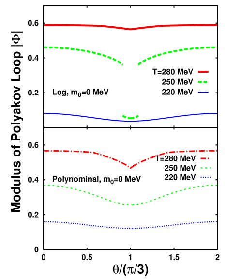
Figure 4: Modulus of Polyakov loop as a function of $\theta$ in the chiral limit. Upper panel: Logarithmic potential, Lower panel: Polynomial potential. The temperatures are the same as in Fig. 3.

IV.1 Behavior across $\theta=\pi/3$

We now consider the order parameter as a function of $\theta$ close to $\theta=\pi/3$. In Figure 3 we show the phase of the Polyakov loop $\phi$ as a function of $\theta$ in the chiral limit. We do not show results for non-zero quark mass, since the results are indistinguishable from those shown in Fig. 3.

At low temperatures (arrow A in Fig. 1), the phase of the Polyakov loop changes smoothly from 0 at $\theta=0$ to $-\pi/3$ at $\theta=\pi/3$. Subsequently, the phase continues to decrease and finally approaches to $-2\pi/3$ at $\theta=2\pi/3$, as required by the symmetry, Eq. (16). This behavior is independent of the choice of $\mathcal{U}$. At temperatures beyond $T_{E}$, the transition is first order (arrow C in Fig. 1). For instance at $T=280$ MeV, the phase jumps from $\phi=0$ to $-2\pi/3$ at $\theta=\pi/3$. This is the Roberge-Weiss transition Roberge and Weiss (1986), where the phase of the Polyakov loop jumps from one $Z(3)$ sector to another. The RW transition is common to both parametrizations of $\mathcal{U}$. This is natural, since the RW transition is a consequence of of the $Z(3)$ symmetry of the pure gauge theory, which is incorporated in both potentials. The detailed behavior around $T_{E}$ is, however, different between the two potentials. Thus, at $T=250$ MeV for the logarithmic potential, which is below the endpoint of the RW transition ($T_{E}\simeq 255$ MeV), the phase is discontinuous at $\theta\neq\pi/3$. This implies that the phase boundary, which is crossed by arrow B in Fig. 1, is first order at this temperature. By contrast, in the polynomial case the phase is a smooth function of $\theta$ at any temperature below the RW endpoint ($T_{E}\simeq 275$ MeV). As we discuss below, this reflects the different order of the RW endpoint for the two potentials.

We note that the logarithmic potential is defined in a limited domain, characterized by positivity of the argument of the logarithm, while for the polynomial potential there is no such restriction. In fact, for high temperatures (e.g. $T=280$ MeV) the Polyakov loop, plotted for the polynomial potential as a function of $\theta$ in the complex $\Phi$ plane, leaves the so called target space, defined by requiring that the logarithmic potential is real Wozar et al. (2006).

In Figure 4 we show the modulus of the Polyakov loop $|\Phi|$ as a function of $\theta$. At high temperatures, the RW transition is manifested by a cusp at $\theta=\pi/3$, while at lower temperatures $|\Phi|$ varies smoothly for both parametrizations of the Polyakov-loop potential. However, at intermediate temperatures, the two potentials yield qualitatively different results, as illustrated by the discontinuities in $|\Phi|$ obtained for the logarithmic potential near $\theta=\pi/3$ at $T=250$ MeV. For the polynomial potential we find a continuous confinement-deconfinement transition at imaginary chemical potential, while for the logarithmic potential the transition is first order at intermediate temperatures. We return to this point in the following subsection. Here we note only that the first order transition is reflected also in a sudden change of the phase at $T=250$ MeV, as shown in Fig. 3.

Within the PNJL model, the transition from one $Z(3)$ sector to another can be understood in the following way. In the high temperature limit, the dominant contribution to the thermodynamic potential is given by the single quark excitation term in Eq. (24) (the first term in the square bracket), which yields a contribution to $\Omega\sim-\cos(\theta+\phi)$. The only additional $\phi$-dependent term in $\Omega$ is the Polyakov loop potential $\mathcal{U}$. At high temperature, $\mathcal{U}$ has the three local minima at $\phi=0$ and $\pm 2\pi/3$. For each value of $\theta$, the physical vacuum is obtained by finding the absolute minimum of the two terms. As illustrated in Fig. 5, the physical vacuum changes from one minimum to the next as $\theta$ crosses $\pi/3+2\pi k/3$. While both potentials have the periodicity $\Delta\theta=2\pi$, when $\phi$ is artificially fixed in one $Z(3)$ sector, the complete thermodynamic potential acquires the periodicity $\Delta\theta=2\pi/3$ owing to the $\phi$ dependence of $\mathcal{U}$.

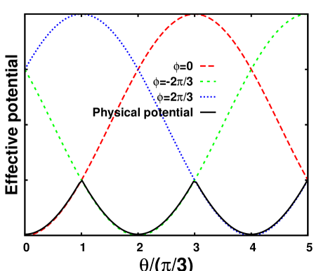
Figure 5: Schematic effective potential for the RW transition.

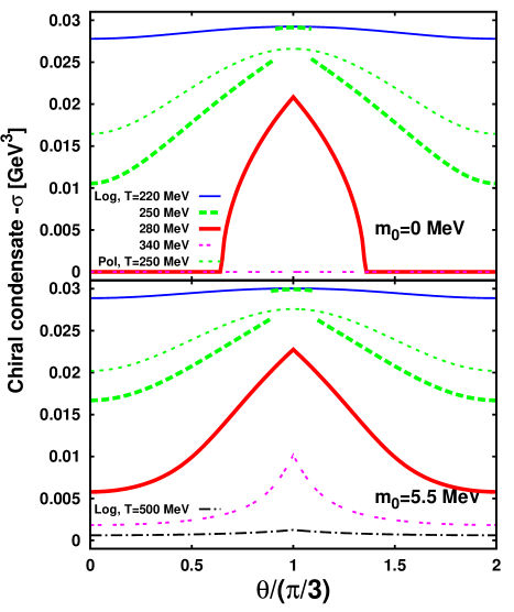
Figure 6: Chiral condensate at various temperatures as a function of $\theta$ in the chiral limit. The temperatures associated with the lines are the same as Fig. 3.

Similarly, the chiral condensate $\sigma$ is also continuous near $\theta=\pi/3$ at temperatures lower than $T_{E}$, irrespective of the quark mass and the potential, as shown in Fig. 6. At temperatures higher than $T_{E}$, it develops a cusp for both parametrizations, a manifestation of the RW transition. Furthermore, at temperatures above $T_{\chi}(\theta=\pi/3)$, $\sigma$ vanishes for any value of $\theta$ in the chiral limit, as shown for $T=340$ MeV. For a finite quark mass, the cusp persists to temperatures much higher than $T_{\chi}$ but finally disappears, as shown in Fig. 6 for $m_{0}=5.5$ MeV and $T=500$ MeV.

In the chiral limit, for temperatures in the interval between $T_{\chi}(\theta=0)$ and $T_{\chi}(\theta=\pi/3)$, there is a second order chiral transition at non-zero $\theta$, as shown in Fig. 6, (see also arrow B in Fig. 1). For finite quark masses, this transition is of the cross-over type, as illustrated in the lower panel of Fig. 6 for $m_{0}=5.5$ MeV. Also the temperature dependence of $\sigma$ is clearly different for the two potentials. In particular, there is a discontinuity in $\sigma$ near $\theta=\pi/3$ at $T=250$ MeV for the logarithmic potential. The values of temperature and imaginary chemical potential corresponding to the discontinuity are identical to the ones obtained for the Polyakov loop.

Figure 7: Behavior of the order parameters around a first order phase transition point in the chiral limit. We depict $T=250$ MeV. From top to bottom, each panel shows the chiral condensate, modulus of the Polyakov loop, and the phase of the Polyakov loop. The vertical line (thin dashed) show the critical $\theta$, determined by a Maxwell construction.

IV.2 First-order phase transition at $T<T_{E}$

In this section we focus on the first order transition found in a limited temperature range below the Roberge-Weiss transition for the logarithmic potential. In Fig. 7 we illustrate this result at $T=250$ MeV. In each panel two lines are shown: one is the solution of the gap equations approaching the transition from small $\theta$, while the other is obtained by approaching from the opposite side.

The existence of two solutions in a certain range of $\theta$ shows that there are two local minima in the thermodynamic potential. The first-order phase transition takes place at the value of $\theta$, where the thermodynamic potential in the two local minima is degenerate. At $T=250$ MeV, this happens at $\theta=0.911(\pi/3)$. The lines terminate where the corresponding minimum disappears. Thus, the system exhibits hysteresis, a characteristic of a first-order phase transition.

Although this transition is related to the confinement-deconfinement transition, the discontinuity is reflected also in the chiral condensate $\sigma$, owing to the coupling between the Polyakov loop and the chiral order parameter.

IV.3 The RW endpoint

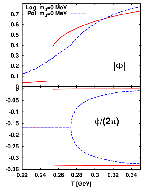
Figure 8: Behavior of $|\Phi|$, and $\phi$ as functions of $T$ at $\theta=\pi/3$.

The existence of the first-order transition, discussed in the previous section, is closely related to the characteristics of the RW endpoint. In Fig. 8 we show the temperature dependence of the Polyakov loop along the line $\theta=\pi/3$ (cf. Fig. 1) for the two potentials in the chiral limit. The nature of the RW endpoint, as characterized e.g. by the phase of the Polyakov loop, differs between the two potentials. While the polynomial potential yields a continuous transition, the logarithmic one exhibits a discontinuity in the phase and magnitude of the Polyakov loop.

Above the RW endpoint ($T=T_{E}$), the phase of the Polyakov loop can take two values on the $\theta=\pi/3$ line, corresponding to different $Z(3)$ sectors (cf. Fig. 5). Thus, in the case of the polynomial potential, the phase bifurcates smoothly at the RW endpoint, while for the logarithmic potential, the phase changes discontinuously at this point. In the former case, the RW endpoint is a second order point, while in the latter it is a triple point. We note, however, that a different parameterization for the logarithmic potential Fukushima (2004) also yields a second order RW endpoint Kouno et al. (2009).

Consequently, the characterization of the RW endpoint depends on the parametrization of the Polyakov loop potential, but, within the framework considered here, it is independent of the value for the quark mass for the logarithmic potential. On the other hand, in LGT calculations it is found that the nature of the RW endpoint depends crucially on the quark mass; for both two and three flavor QCD it is a second order endpoint at intermediate quark masses and a triple point for large and small masses de Forcrand and Philipsen (2010); Bonati et al. (2011). In Ref. Sakai et al. (2010a) it is argued that in order to reproduce the quark mass dependence of the RW transition, a $\Phi$ dependent fermion coupling, motivated by functional renormalization group analyses Kondo (2010); Braun et al. (2011), is required. This indicates that in QCD the interplay between chiral symmetry breaking and confinement is more complicated than in the present model.

Figure 9: Phase diagram for the logarithmic potential (top) and the polynomial potential (bottom).

Finally, in Fig. 9 we summarize the results on the phase diagram in the $T-\theta$ plane for the two Polyakov loop potentials. The (pseudo-)critical temperature for the deconfinement transition corresponds to a maximum of the temperature derivative of the modulus of the Polyakov loop $d|\Phi|/dT$. The critical end point (CEP), obtained for the logarithmic potential at $0<\theta<\pi/3$, is a consequence of the triple point at $T=T_{E}$ and $\theta=\pi/3$.

In comparison of the two potentials, we have seen that the phase transitions at imaginary chemical potential are shifted to higher temperatures compared to those at real chemical potential. This implies that dynamical quark mass becomes heavier at fixed temperature (see Fig. 6) thus the Polyakov loop potential $\mathcal{U}$, which is independent of $\theta$, makes a dominant contribution to the thermodynamic potential. Furthermore, at imaginary chemical potential, the target space of the Polyakov loop is probed through the change of the phase $\phi$. Therefore, a comparison of the resulting phase diagram at the imaginary chemical potential region with that obtained in LGT calculations, yields important constraints on the effective Polyakov loop potential.

IV.4 Critical endpoint of confinement-deconfinement transition

In Ref. Bowman and Kapusta (2009) it was found that as the pion mass in the quark-meson model is reduced from its physical value, an additional critical endpoint appears on the phase boundary at small (real) values of the chemical potential. Since the coupling to the Polyakov loop is not accounted for in Bowman and Kapusta (2009), the additional CEP is associated with the chiral phase transition . In this section we explore the dependence of the confinement-deconfinement CEP, which appears at imaginary $\mu$ for the logarithmic potential, on the model parameters. We find that the location of this CEP depends on the four fermion coupling constant $G_{s}$.

Figure 10: Phase diagrams on $T-\mu^{2}$ plane for various $G_{s}$ in the chiral limit. Solid lines stand for the first order phase transition lines. Dashed lines denote the second or crossover transition. For convenience, $\mu^{2}=0$ and $\mu_{I}/T=\pi/3$ are indicated by the thin and thick dotted lines, respectively. The closed circles show the location of the CEP for the confinement-deconfinement transition.

In Fig. 10 we show the phase diagram of the model in the chiral limit for different values of $G_{s}$. We include both real and imaginary values of $\mu$ by showing the phase boundaries in $T-\mu^{2}$ plane. The upper panels show cases where $G_{s}$ is smaller, while the lower ones show cases where it is larger than the reference value (29). Lines appearing for $\mu^{2}<-(\pi T/3)^{2}$ (the boundary is indicated by the dotted line) are images of those in the region $-(\pi T/3)^{2}\leq\mu^{2}\leq 0$; the mapping is defined by the periodicity of the partition function.

We identify the (pseudo)critical temperature by finding the the maximum of the derivative of the corresponding order parameter with respect to temperature. For real values of the chemical potential, the Polyakov loop and its conjugate are real but take on different values Sasaki et al. (2007). Here we use $d\Phi/dT$ for the definition of the deconfinement transition. A different definition, based e.g. on the Polyakov loop susceptibility Sasaki et al. (2007), would lead to a slightly different value of the pseudocritical temperature of the crossover transition.

For the first order transition at large $\mu^{2}$ one finds double peaks in $d\Phi/dT$ (cf. Fig. 10). Here we identify the position of the transition with the maximum which smoothly extrapolates to the deconfinement transition at vanishing chemical potential and to the chiral transition at $T=0$, where the peak structure is simple. We note that any ambiguity in the location of the phase boundary does not affect the discussion below.

Qualitatively the features of the phase diagram can be classified as follows. The NJL sector has a critical coupling $G_{s}^{\text{cr}}=\pi^{2}/(2N_{c}\Lambda^{2})$ for the gap equation to have a nontrivial solution Hatsuda and Kunihiro (1994). This implies that, with the present three-momentum cutoff, there is no spontaneous breakdown of chiral symmetry for $G_{s}<4.125$ GeV^-2. Therefore, in the upper-left panel ($G_{s}=3.5$ GeV^-2), the system is everywhere in the chirally symmetric phase. In this case the RW endpoint is still a triple point, and the CEP of the deconfinement transition is close by, at $\theta=0.95\pi/3$.

For $G_{s}>G_{s}^{\text{cr}}$, there is a chiral transition at vanishing chemical potential. As seen in the upper-center panel, there is a precursor at imaginary chemical potential for $G_{s}$ slightly smaller than $G_{s}^{\text{cr}}$. The chiral symmetry is spontaneously broken in a small region at intermediate temperatures adjoining the $\mu^{2}=-(\pi T/3)^{2}$ line. This behavior can be understood along the lines presented in Sec. III.2. Although the Boltzmann approximation, Eq. (24), might not be a good approximation since the system is in the chirally symmetric phase even at low temperatures, the Polyakov loop is small so that the thermal contribution is dominated by the $\cos 3\theta$ term as in Eq. (25). Since this term is positive in the $\pi/6<\theta<\pi/2$, it adds to the vacuum term and a non-trivial solution appears at finite temperature where the system enters the broken phase.

As the temperature is increased further, however, the Polyakov loop is non-zero and the one- and two- quark excitations contribute to the gap equation, driving the system back into the symmetric phase. Consequently, near the RW endpoint, the chiral and deconfinement transitions occur simultaneously and the chiral transition is also of first order. Note that the lower endpoint of the chiral transition follows the $\mu^{2}=-(\pi T/3)^{2}$ line and arrives at the origin when $G_{s}=G_{s}^{\text{cr}}$. For $G_{s}$ beyond this value, the chiral transition line enters the $\mu^{2}>0$ half-plane.

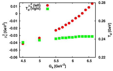
Figure 11: Location of the CEP as a function of $G_{s}$. The left vertical axis shows the chemical potential while the right one denotes the temperature.

As $G_{s}$ is increased beyond $G_{s}=G_{s}^{\text{cr}}$, the location of the deconfinement CEP moves to larger $\mu^{2}$ and finally reaches real values of the chemical potential at $G_{s}\simeq 6.5$ GeV^-2. At the same time, the chiral transition line moves to larger $T$ and $\mu^{2}$. The behavior of the CEP can be directly related to changes of the chiral transition with increasing $G_{s}$. Increasing $G_{s}$ leads to a larger dynamical mass $M=m_{0}-2G_{s}\sigma$ in the chirally broken phase. Moreover, $|\sigma|$ increases with $G_{s}$ since a stronger scalar coupling leads to larger quark condensate. This raises both the dynamical mass and the chiral transition temperature. On the other hand, a modified $G_{s}$ does not alter the Polyakov loop sector of the model. Consequently, near the deconfinement transition, the dynamical mass of the quarks increase with $G_{s}$ and the system approaches a pure gauge theory owing to the thermal suppression of quark degrees of freedom. Thus, as shown in Fig. 11, the first order phase transition of the pure gauge theory is recovered at $G_{s}=6.3$ GeV^-2, only 15% above the reference value (29).

One may wonder why this mechanism is not effective for the polynomial potential, since it also exhibits a first order phase transition in the absence of fermions. In fact, we find that the polynomial potential does show the same behavior, but at much larger values of the scalar coupling. The RW endpoint, which is second order at $G_{s}=5.498$ GeV^-2, is first order transition starting at $G_{s}=12.4$ GeV^-2 and the deconfinement CEP reaches $\mu^{2}=0$ at $G_{s}=25$ GeV^-2, 4.5 times larger than the reference value.

The origin of this quantitative difference between the polynomial and logarithmic potentials is due to the much weaker first order phase transition (smaller discontinuity in $\Phi$) exhibited by the polynomial potential in the heavy quark limit. At $G_{s}=25$ GeV^-2 we find a dynamical quark mass of about 2.5 GeV. Thus, for a quark mass less than 2.5 GeV the first order transition is smoothened to a crossover transition. By contrast, for the logarithmic potential this happens at a much smaller dynamical quark mass of 0.4 GeV, owing to the much stronger underlying first order transition.

We note that a first order confinement-deconfinement transition emerges at real chemical potential also in the large $N_{c}$ limit of the PNJL model McLerran et al. (2009), as explored in the context of the recently proposed quarkyonic phase McLerran and Pisarski (2007). Indeed, the effect of strengthening $G_{s}$ is similar to that of increasing $N_{c}$ since $G_{s}$ and $N_{c}$ appear in the factor $G_{s}N_{c}$ in the gap equation for the dynamical mass (see Eq.(16) in Ref. McLerran et al. (2009)). While we suppress the quark contribution to the thermodynamics by increasing the dynamical mass by means of $G_{s}$, a large value of $N_{c}$ is accompanied by a $1/N_{c}$ suppression of the quark contribution. Both procedures yield a gluon dominated system and thus give a first order confinement-deconfinement transition.

Note, however, that the two procedures differ in detail. Increasing $G_{s}$ at fixed $N_{c}$ preserves the Polyakov loop potential but modifies the quark mass, while in the large $N_{c}$ limit at fixed $G_{s}N_{c}$ the quark mass remains unchanged but the Polyakov loop potential is modified. This means that when we increase $G_{s}$ at fixed $N_{c}$ we change the characteristic scale of the chiral symmetry breaking. Although this does not correspond to the physical situation, since QCD has unique scale, $\Lambda_{\text{QCD}}$, our result could be useful for exploring the interplay between the chiral phase transition and deconfinement.

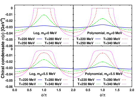
Figure 12: Chiral condensate $\sigma=\langle\bar{q}q\rangle$ as a function of the twisted angle $\varphi$.

V Dual parameter for the confinement-deconfinement transition

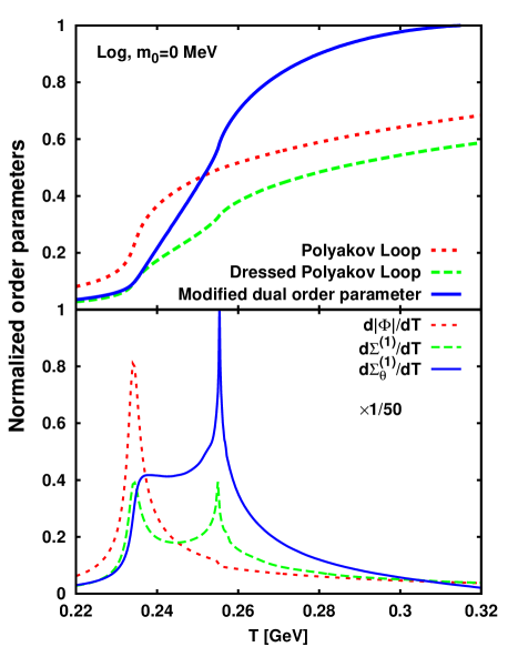
Figure 13: Characteristic parameters (upper) and their derivatives with respect to temperature (lower) for the confinement-deconfinement transition in the chiral limit for the logarithmic potential.

Figure 14: Same as Fig. 13, but for the polynomial potential.

In this section, we consider dual parameters which capture the characteristic feature of the confinement-deconfinement transition discussed above. Recently a dual parameter has been introduced by considering a generalized boundary condition for fermions

$$q(\boldsymbol{x},\beta)=e^{i\varphi}q(\boldsymbol{x},0).$$ (31)

Here $\varphi$ is so-called the twisted angle. The dual quark condensate $\Sigma^{(n)}$ is defined as the $n$-th Fourier coefficient of the chiral condensate as a function of the twisted angle Bilgici et al. (2008)

$$\Sigma^{(n)}(T)=-\int_{0}^{2\pi}\frac{d\varphi}{2\pi}e^{-in\varphi}\sigma(T,\varphi).$$ (32)

The chiral condensate $\sigma(T,\varphi)$ is defined in terms of $\varphi$ by Bilgici et al. (2008)

$$\sigma(\varphi)=-\frac{1}{V}\langle\text{Tr}[(m_{0}+D_{\varphi})^{-1}]\rangle_{G}.$$ (33)

In Ref. Bilgici et al. (2008), this quantity was introduced based on the lattice regularization. The $\varphi$ dependence of $\text{Tr}[(m_{0}+D_{\varphi})^{-1}]$ can be written down explicitly by using the link variable. It reduces to the ordinary chiral order parameter in the limit of $m\rightarrow 0$ and $V\rightarrow\infty$. An implementation in the continuum theory has been done in the framework of Dyson-Schwinger equation Fischer and Mueller (2009). The most interesting quantity is that of $n=1$, which is called dressed Polyakov loop. Because of a relation to the ordinary Polyakov loop, it can be regarded as an order parameter of the confinement-deconfinement transition.

Figure 15: Same as Fig. 13, but for $m_{0}=5.5$ MeV.

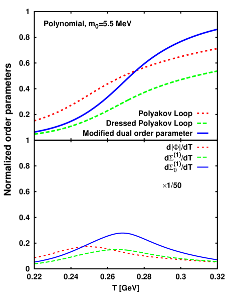
Figure 16: Same as Fig. 14, but for $m_{0}=5.5$ MeV.

From the fermionic boundary conditions (31), one immediately finds that this is equivalent to introducing the imaginary chemical potential [Eq. (5)]. The only difference is that $\varphi=\pm\pi$ corresponds to the usual anti-periodic boundary condition in the twisted angle while $\theta=0$ does so in the imaginary chemical potential. In this case, the relation between $\varphi$ and $\theta$ is given by just a shift of $\pm\pi$,

$$\varphi=\theta\pm\pi\quad(\text{mod}\quad 2\pi/N_{c}).$$ (34)

Furthermore, one notes that the dual condensate (32) is quite similar to the canonical partition function (1).

However, the LGT calculations demonstrate that $\sigma(\varphi)$ exhibits quite different behavior from that for the imaginary chemical potential Bilgici et al. (2010). $\sigma(\varphi)$ shows a periodicity of $2\pi$ in $\varphi$, not $2\pi/3$ which is required by the RW periodicity. The origin of this difference is the expectation value of the operator $\langle\cdots\rangle_{G}$ in Eq. (33). The subscript $G$ denotes the path integral over the gauge field with the fermion determinant which follows the ordinary boundary condition. The change of the boundary condition (31) applies only to the Dirac operator. In the case of the imaginary chemical potential, different $\theta$ gives a different fermion determinant while in the case of the twisted angle the background field does not change with the boundary condition. Therefore $\varphi$ dependence of the chiral condensate differs from $\theta$ dependence. In a PNJL model, the authors of Ref. Kashiwa et al. (2009) use the value of the Polyakov loop calculated at $\theta=0$ to obtain the chiral condensate $\sigma(\varphi)$. This prescription corresponds to varying only the fermionic boundary condition without changing gluonic background. We will follow the same prescription below. Since the periodicity $2\pi/3$ in the imaginary chemical potential is preserved by the RW transition, which is an effect of the Polyakov loop in the context of PNJL model, the relation (34) holds for the normal NJL model calculation which does not couple to $Z(3)$ field. In spite of the absence of confinement in the NJL model, one sees that behavior of the dual chiral condensate is quite similar to one obtained from lattice QCD and PNJL model Mukherjee et al. (2010).

Figure 12 shows the chiral condensate as a function of the twisted angle $\varphi$, obtained by the same method as used in Ref. Kashiwa et al. (2009). The periodicity is no longer $2\pi/3$. One also notes that there is broken phase at region far from $\varphi=\pi$ even at high temperatures. This is in contrast to the case of the imaginary chemical potential shown in Fig. 6 and similar to what was expected from the gap equation of the NJL model, Eq. (28). Indeed, at $\varphi=\pi/2$ and $3\pi/2$, which correspond to $\theta=\mp\pi/2$, the thermal term vanishes in Eq. (28), resulting in the almost temperature indepedent chiral condensate. On the other hand, there are no qualitative difference between the logarithmic potential and the polynomial one. The reason is that the Polyakov loop enters in the gap equation only as a constant determined at $\varphi=\pi$ at each temperatures.

Let us introduce a new dual parameter by using $\theta$ instead of $\varphi$ such that it captures the characteristics in the $\theta$ space. We define

$$\Sigma_{\theta}^{(n)}(T)\equiv\frac{3}{2\pi}\intop_{-\pi/3}^{\pi/3}d\theta e^{-in\theta}\sigma(T,\theta).$$ (35)

The integration region is changed to $[-\pi/3:\pi/3]$ with respect to the periodicity $2\pi/3$. As discussed in Sec. III.2, the physical meaning of the periodicity is different in confinement and deconfinement phase. In the confinement phase, periodicity $2\pi/3$ is coming from $\cos 3\theta$ which characterizes the confinement of the quarks. On the other hand, deconfinement phase is characterized by $\cos\theta$ with discontinuity at $\theta=\pi/3+2\pi k/3$ caused by $Z(3)$ transition which preserves the periodicity $2\pi/3$. Therefore, we expect, that $\Sigma_{\theta}^{(1)}$ and $\Sigma_{\theta}^{(3)}$ demonstrate characteristic behavior of the confinement-deconfinement transition.

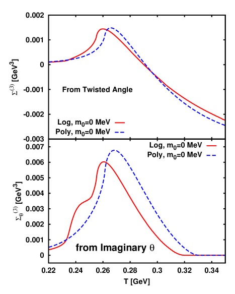
Figure 17: Dual order parameters of $n=3$. Upper panel shows the result from Eq. (32) while lower one displays that from Eq. (35).

In Figs. 13 and 14, we compare the three kinds of the characteristic parameters of the confinement-deconfinement transition and their derivatives with respect to temperature as functions of temperature. We normalized the dressed Polyakov loop and the modified dual parameter (35) so that they tend to 0 at low temperature and to unity at high temperature by $\Sigma_{\text{norm}}(T)\equiv[\Sigma(T)-\Sigma(T_{1})]/[\Sigma(T_{2})-\Sigma(T_{1})]$ where we used $T_{1}=50$ MeV and $T_{2}=1$ GeV. The same normalization constants are applied to the derivatives. Note that $\Sigma_{\theta}^{(n)}$ before normalization vanishes at temperature higher than the chiral transition temperature at $\theta=\pi/3$ in the chiral limit since $\sigma(T,\theta)$ does so, as seen in Fig. 6. After the normalization, it smoothly approaches to unity as one sees in Figs. 13–16.

One observes qualitatively that both dual parameters show similar behavior to the Polyakov loop. The dressed Polyakov loop is almost parallel to the Polyakov loop in the temperature region covered in the figure. On the other hand, the modified dual parameter $\Sigma_{\theta}^{(1)}$ reaches quickly its limiting value. The behavior around the transition temperatures reflect the difference between two potentials. In the case of the logarithmic potential, one sees different structures for each derivative of the order parameters. While the derivative of the Polyakov loop $d|\Phi|/dT$ shows the only peak corresponding to the pseudocritical temperature, the dressed Polyakov loop $d\Sigma^{1}/dT$ exhibits the two peak structure. One agrees with that of the $d\Phi/dT$ and the other corresponds to the chiral transition (see Fig. 2). The derivative of the modified dual parameter $d\Sigma_{\theta}^{(1)}/dT$ also shows a peak for the chiral transition. However, the deconfinement appears only as a shoulder. The polynomial potential shows a broader peak in $d\Phi/dT$ reflecting the weaker nature of transition. However, maxima in dual order parameters associated with the crossover transition do not appear.

Inclusion of small quark mass, $m_{0}=5.5$ MeV slightly modifies the behavior of the characteristic parameters, as expected from the difference in $\sigma$. Figures 15 and 16 show the three parameters and their derivatives for $m_{0}=5.5$ MeV. While at finite quark mass there is little difference in the behavior of the parameters seen in $m_{0}=0$ case, distinct peak structures show up in their derivatives. For the logarithmic potential, the peak associated with the chiral transition seen in the chiral limit does not exist in both dual parameters. The remnant of the chiral transition appears only in the modified dual parameter as a dip. On the other hand, polynomial potential case exhibits much broader peak, which corresponds to deconfinement in $d|\Phi|/dT$ and to chiral transition in dual parameters.

Figure 17 shows the dual parameter (32) and (35) at $n=3$. In all the cases, one sees that they start to increase, exhibit peak structure and then decreasing. This is common for both $\Sigma^{(3)}$ and $\Sigma_{\theta}^{(3)}$. Such behavior of $\Sigma_{\theta}^{(3)}$ can be understood by analysing $\sigma(T,\theta)$ which is shown in Fig. 6. At low $T$, it oscillates according to $\cos 3\theta$ with an amplitude given by the thermal factor. Then $\Sigma_{\theta}^{(3)}$, which is proportional to the amplitude, increases with $T$. At $T>T_{\chi}$, $\sigma(\theta,T)$ vanishes at $\theta=[0:\theta_{c}]$ thus only the region $[\theta_{c}:\pi/3]$ contributes to the integral. Therefore, $\Sigma_{\theta}^{(3)}$ has a peak at $T=T_{\chi}$ and then decreases. This does not relate to the deconfinement phenomenon and is common for $\Sigma^{(3)}$ and $\Sigma_{\theta}^{(3)}$.

If one focuses on the difference between the logarithmic an the polynomial potential, however, one finds a remnant of the deconfinement-confinement transition in the behavior of $\Sigma_{\theta}^{(3)}$. As we have seen in Fig. 7, $\sigma(T,\theta)$ has a discontinuity induced by the first-order confinement-deconfinement transition. It is reflected to the non-monotonic behavior of $\Sigma_{\theta}^{(3)}$ between $T=0.24$ and $T=0.26$ GeV in the case of logarithmic potential. Indeed, the shoulder seen at $T=0.24$ GeV corresponds to the temperature of CEP, at which $\sigma(\theta,T)$ has a discontinuity, and the second inflection point reflects the RW endpoint which is the triple point in this case. This indicates that the newly introduced dual parameter $\Sigma_{\theta}^{(3)}$ has sensitivity to the confinement-deconfinement transition at imaginary chemical potential.

VI Summary

We have studied the confinement-deconfinement transition in the PNJL model at imaginary chemical potential with the simplest interaction. We discussed the origin of the characteristic periodicity $2\pi/3$ of the order parameters. It is characterized by $\cos 3\theta$ in the confined phase while it is due to $\cos\theta$ with the RW transition at $\theta=\pi/3+2\pi k/3$ induced by the change of the phase of the Polyakov loop. We also explored the results from different Polyakov loop potentials. We found that the property of the confinement-deconfinement transition depends on the choice of the potential in spite of the fact that both potentials exhibit the first-order phase transition in the absence of quarks. Remarkable differences are seen in both the RW endpoint and the behavior of the Polyakov loop at finite $\theta$. In the case of the logarithmic potential which has more relevant domain, we find that the confinement-deconfinement transition becomes first order near $\theta=\pi/3$ and there is a critical endpoint of the transition at imaginary chemical potential. We also find that the location of the CEP moves with the four fermion coupling $G_{s}$ and it reaches real chemical potential region by increasing $G_{s}$. This behavior can be understood by the suppression of the quark contribution since increasing $G_{s}$ implies larger $\langle\bar{q}q\rangle$ which quantifies the dynamical quark mass. At large coupling, the existence of the CEP is independent of the choice of the potential. However, the polynomial potential requires larger $G_{s}$ because it exhibits much weaker first order transition. Consequently, it seems that the order of the deconfinement transition is determined by the size of the gap $\Delta\Phi$ in the Polyakov loop potential and the quark condensate $\langle\bar{q}q\rangle$.

The first order phase transition influences the behavior of the chiral condensate as a sudden jump at the critical imaginary chemical potential. We proposed modified dual parameters using the imaginary chemical potential based on the analogy to the twisted angle in the dual order parameters. Comparing the $n=1$ case with the Polyakov loop and the dressed Polyakov loop, we found that each parameters has different sensitivity to the phase transitions. We showed that $n=3$ has a characteristic behavior owing to the first order confinement-deconfinement transition at intermediate $\theta$. We expect relevance of our study in understanding the QCD phase diagram.