EVOLUTION OF NON-GAUSSIANITY IN MULTI-SCALAR FIELD MODELS

Abstract

We study the evolution of non-Gaussianity in multiple-field inflationary models, focusing on three fundamental questions: (a) How is the sign and peak magnitude of the non-linearity parameter $f_{\mathrm{NL}}$ related to generic features in the inflationary potential? (b) How sensitive is $f_{\mathrm{NL}}$ to the process by which an adiabatic limit is reached, where the curvature perturbation becomes conserved? (c) For a given model, what is the appropriate tool – analytic or numerical – to calculate $f_{\mathrm{NL}}$ at the adiabatic limit? We summarise recent results obtained by the authors and further elucidate them by considering an inflection point model.

PACS numbers: 98.80.-k, 98.80.Cq

1 Introduction

An important feature of canonical single field models is that the curvature perturbation produced at horizon crossing is conserved,[2, 1] with statistics indistinguishable from Gaussian.[3] In multiple field models, on the other hand, isocurvature modes may also be produced, and can subsequently source the evolution of the curvature perturbation as the field space path curves.[4, 5] The curvature perturbation and its statistics (such as the power spectrum and non-Gaussianity[6, 7]) can therefore continuously evolve after horizon crossing, leading to far richer behaviour than that allowed in single field models. Here we focus on non-Gaussianity, and in particular the nonlinearity parameter, $f_{\mathrm{NL}}$, though many of our general conclusions extend to other observables as well.

In canonical multi-field models, the non-Gaussianity present at horizon crossing is negligible.[8] In this setting, however, it is possible for $f_{\mathrm{NL}}$ to evolve to large values.[9, 10, 11, 12] To calculate the observationally relevant value of non-Gaussianity, in principle one has to follow the evolution until the time of last scattering, where the Cosmic Microwave Background (CMB) was imprinted. Given our present ignorance about the detailed physics of the early universe, this would not be possible in practice. In many models, however, a regime is reached during the evolution long before this time – the so-called adiabatic limit – where all the isocurvature modes decay, and the curvature perturbation becomes conserved.

There are different ways in which such a limit could be reached, and this has consequences both for the possible values of the observable parameters, such as $f_{\mathrm{NL}}$, and for the techniques which can be reliably employed to calculate observables, i.e. whether analytic methods will suffice, or numerical methods are necessary. A useful classification of models according to when the adiabatic limit is attained is:

• Models in which an adiabatic limit is reached ‘naturally’ by convergence into a ‘focusing region’ of the potential. This can be further sub-divided into cases where the convergence occurs during slow-roll, and cases in which convergence occurs only after the slow-roll approximation fails.

• Models where an adiabatic limit is reached abruptly due to an additional degree of freedom, such as a waterfall field being destabilised.

• Models for which no focusing region in the inflationary potential exists, and an adiabatic limit can be reached only by embedding the inflationary model into a larger scenario, perhaps one which includes perturbative reheating.

Recently an extended study of these possibilities was undertaken by the authors in the context of of multi-field models of inflation, capable of producing large non-Gaussianities.[13] Here we give a summary of those results and further elucidate them by considering an inflection point model, which is of the first type, and which can produce a large positive or negative value of $f_{\mathrm{NL}}$ at the adiabatic limit.

The structure of the paper is as follows. In §2 we give a summary of the background theory which is used to formulate analytic expressions for observables, discussed in §3, together with the conditions needed for the non-Gaussianity to be large at the adiabatic limit when it is reached naturally. In §4 we briefly discuss features in the potential which generate large transitory non-Gaussianities during the super-horizon evolution, which may be relevant for the final observable value at the adiabatic limit if this limit is reached abruptly. Finally, we discuss the usefulness of our results in §5 when applied to specific models, and demonstrate this by considering a new example. We conclude in §6.

2 Background

We consider inflation driven by multiple canonical scalar fields $\phi_{i}$ with $i=1,2,...,\,{\cal M}$, self-interacting through a potential $W(\phi_{1},\phi_{2},...)$. Defining $W_{,i}={\partial W}/{\partial\phi_{i}}$ the scalar equations of motion are

$$\ddot{\phi}_{i}+3H\dot{\phi}_{i}+W_{,i}=0\,,$$ (1)

where $H$ is the Hubble rate, given by the associated Friedmann equation $3M_{\rm pl}^{2}H^{2}=W+\sum_{i}\dot{\phi}_{i}^{2}/2$. We define slow-roll parameters as

$$\epsilon_{i}=\frac{M_{\rm pl}^{2}}{2}\left(\frac{{W_{,i}}}{W}\right)^{2},~{}~{}~{}\epsilon=\sum_{i=1}^{\cal M}\epsilon_{i},~{}~{}~{}\eta_{ij}={M_{\rm pl}^{2}}\left(\frac{W_{,ij}}{W}\right)\,,$$ (2)

such that for inflation we require $\epsilon<1$. The ‘slow-roll limit’ is given by $\epsilon\ll 1$, during which the fields’ kinetic energy may be neglected, the decaying modes discarded, and the field equations well approximated by

$$3H\dot{\phi}_{i}+W_{,i}=0,~{}~{}~{}~{}3M_{\rm pl}^{2}H^{2}=W.$$ (3)

Primordial cosmological perturbations are commonly characterised in terms of the curvature perturbation on uniform density spatial hypersurfaces, denoted by $\zeta$. An important feature of $\zeta$ is that for adiabatic perturbations it is conserved on large scales,[1] at the linear order and even beyond. In multi-field models, on the other hand, $\zeta$ can evolve due to the presence of isocurvature modes, and this may result in the production of large non-Gaussianities. Deviation of the three-point function from zero is commonly measured in terms of the dimensionless parameter $f_{\mathrm{NL}}$

$$f_{\mathrm{NL}}=\frac{5}{6}\frac{k_{1}^{3}k_{2}^{3}k_{3}^{3}}{k_{1}^{3}+k_{2}^{3}+k_{3}^{3}}\frac{{\cal B}_{\zeta}(k_{1},k_{2},k_{3})}{4\pi^{4}{\cal P}_{\zeta}^{2}},$$ (4)

where ${\cal P}_{\zeta}$ is the power spectrum and ${\cal B}_{\zeta}$ the bispectrum, given respectively by

$$\langle\zeta_{\mathbf{k}_{1}}\zeta_{\mathbf{k}_{2}}\rangle \equiv (2\pi)^{3}\delta^{3}({\mathbf{k}_{1}}+{\mathbf{k}_{2}})\frac{2\pi^{2}}{{k_{1}}^{3}}{\cal P}_{\zeta}(k_{1})\,,$$ (5)

$$\langle\zeta_{\mathbf{k}_{1}}\,\zeta_{\mathbf{k}_{2}}\,\zeta_{\mathbf{k}_{3}}\rangle \equiv (2\pi)^{3}\delta^{3}({{\mathbf{k}_{1}}+{\mathbf{k}_{2}}+{\mathbf{k}_{3}}}){\cal B}_{\zeta}(k_{1},k_{2},k_{3})\,.$$ (6)

A common technique for calculating $\zeta$ and its statistics, including $f_{\mathrm{NL}}$, is the $\delta N$ formalism,[14, 15, 17] based on the separate universe approach to perturbation theory.[2, 16] In this approach, spatial gradients are neglected on scales greater than the horizon size, and each spatial point is assumed to evolve as a separate FRW universe. In phase space, this can be represented by a bundle of trajectories, each evolving along an independent path from perturbatively different initial conditions. The variables which parametrise this phase space are the scalar fields $\{\phi_{i},\dot{\phi_{i}}\}$, as well as any radiation or matter species that may be present. The idea of associating inflationary perturbations with trajectories has a long history.[2, 14, 4, 18]

In this picture, choosing a different spatial slicing of the universe corresponds to taking a different cross section of the bundle in phase space.

Choosing a flat initial slicing at $t=t^{*}$, and a later uniform density (constant $H$) slicing at $t=t_{c}$, then $\zeta$ on the final slicing can be equated with the difference in the number of e-folds, as measured along different trajectories in the bundle, $\zeta=\delta N$.

In general, as the bundle evolves in the field space, so will $\delta N$ and its statistics, requiring the dynamics to be followed indefinitely. If, however, the trajectories converge to a line parametrised by a single variable, i.e. the adiabatic limit, $\zeta$ becomes conserved. Moreover, in this limit each value of the Hubble rate corresponds to a single combination of the field or fluid content, implying that derivatives of final quantities on $c$, with respect to changes in the initial conditions, tend to zero as the adiabatic limit is reached. In particular, one finds $\partial\phi_{i}^{c}/\partial\phi_{k}^{*}\to 0$.

Restricting our attention to purely scalar field dynamics, a common example of how an adiabatic limit is reached is for the trajectories to evolve into a focusing region of the potential, such as a potential valley, possibly terminating in a minimum. For convergence into a valley, the mass-squared matrix associated with perturbations orthogonal to the direction to which the trajectories are converging should have large and positive eigenvalues. Taking the smallest eigenvalue to be of magnitude $\sim m_{\perp}$, one typically expects a decay of the field derivatives $\partial\phi_{i}^{c}/\partial\phi_{k}^{*}$ at least as fast as $e^{-(m_{\perp}N)/(3H)}$ (see our recent work[13] for a detailed discussion). As was mentioned in the introduction, however, an adiabatic limit could be reached in other ways. It may turn out that no focusing region in the potential is available, in which case the decay of the fields into radiation may need be considered in order for the model to make unambiguous predictions. Alternatively, an adiabatic limit could occur due to a sudden transition, such as a waterfall field being destabilised.

In any case, before we can consider the fate of observables at the adiabatic limit, it is first necessary to have calculable expressions for these quantities, which could be obtained using the $\delta N$ formalism discussed above. We recall that during slow-roll inflation field velocities are functions of field positions. Taking this to be a good approximation at horizon crossing, the subsequent number of e-folds undergone by any ‘separate universe’ is then a function purely of the initial field values, $N(\phi_{1}^{*},...,\phi_{\cal M}^{*})$, even if the evolution subsequently evolves away from slow roll. Taking $t^{*}$ as a time shortly after observable scales left the horizon, therefore, a Taylor expansion

$$\zeta\equiv\delta N=\sum_{i}N_{,i}\delta\phi_{i}^{*}+\frac{1}{2}\sum_{ij}N_{,ij}\delta\phi_{i}^{*}\delta\phi_{j}^{*}+\dots$$ (7)

can be made, where $N$ is the number of e-folds from $*$ to $c$, a subscript $i$ represents a derivative with respect to $\phi^{*}_{i}$, and $\delta\phi_{k}^{*}$ are the field fluctuations on the flat hyper-surface at horizon crossing. Such a Taylor series allows the properties of a bundle of trajectories to be parametrised by just a few numbers, namely the derivatives of $N$ about some typical member of the bundle. Moreover, Eq. (7) allows various statistics to be estimated. In particular $f_{\mathrm{NL}}$ is given by[17]

$$f_{\mathrm{NL}}=\frac{5}{6}\frac{\sum_{i,j}N_{,i}N_{,j}N_{,ij}}{\left(\sum_{i}N_{,i}^{2}\right)^{2}}.$$ (8)

3 Analytic Schemes and $f_{\mathrm{NL}}$ at a ‘Natural’ Adiabatic Limit

To analytically evaluate the non-linearity parameter $f_{\mathrm{NL}}$ from Eq. (8) we must calculate $N_{,i}$ and $N_{,ij}$ at time $t^{c}$, or when they become constant at the adiabatic limit. Currently, analytic calculation is only possible when the slow-roll equations of motion, Eq. (3), are a good approximation. This means that if $\zeta$ is still evolving at the end of inflation, we cannot analytically follow observable quantities, and numerical simulations will become essential. Moreover, calculations require a special ‘separable’ form for the potential[4]. Vernizzi & Wands[6] and later Battefeld & Easther[19] studied sum-separable models, $W=\sum_{i}V_{i}(\phi_{i})$, deriving expressions for these coefficients and for $f_{\mathrm{NL}}$. Similar techniques were used by Choi et al.[20] for models of product-separable form $W=\Pi_{i}V_{i}(\phi_{i})$, and recently Wang[21] generalised the study of sum-type potentials to those of the form $W=(\sum_{i}V_{i}(\phi_{i}))^{1/A}$, where $A$ is an arbitrary constant A summary of analytic expressions for ${\cal M}$-field models of these forms is given in our paper.[13]

The analytic formulae follow by using Eq. (3) to write $N$ as an integral over one of the fields $\phi_{k}$ as $N=-\int_{\phi^{*}}^{\phi^{c}}\!\!W/(M_{\rm pl}^{2}W_{,\phi_{k}})\,{\rm d}\phi_{k}$. In general, taking the derivative of this expression yields three contributions, namely initial and final boundary terms and a path term. For potentials for which analytic progress is possible, however, the path terms are either absent, or the integrals can be manipulated to make them so. For potentials with product-separable forms one finds

$$N^{(k)}_{,i}=\left.\frac{V_{k}}{M_{\rm pl}^{2}V_{k}^{\prime}}\right|_{*}\delta_{ik}-\left.\frac{V_{k}}{M_{\rm pl}^{2}V_{k}^{\prime}}\right|_{c}\frac{\partial\phi_{k}^{c}}{\partial\phi_{i}^{*}}\,,$$ (9)

where the free index $k$ labels the ${\cal M}$ ways of writing $N_{,i}$, all of which will lead to the same result once the $c$-dependent terms are evaluated. The summation convention is not used anywhere in this paper. For potentials of generalised sum separable form one finds a similar expression

$$N_{,i}=A\left[\left.\frac{V_{i}}{M_{\rm pl}^{2}V_{i}^{\prime}}\right|_{*}-\sum_{k=1}^{\cal M}\left.\frac{V_{k}}{M_{\rm pl}^{2}V_{k}^{\prime}}\right|_{c}\frac{\partial\phi_{k}^{c}}{\partial\phi_{i}^{*}}\right]\,.$$ (10)

In both cases $N_{,ij}$ follows by differentiation.

The difficult step in deriving an analytic expression for $N_{,i}$ is the calculation of the $c$-dependent derivatives in Eqs. (9)–(10). A case where analytic progress is much easier occurs if the adiabatic limit is reached during slow-roll inflation. If this limit is reached by convergence into a valley,[13] we expect the $c$-dependent derivatives to tend to zero at least as fast as the lightest isocurvature mode decays.[13] If sufficient time is available for them to become negligible, this greatly simplifies the expressions for $N_{,i}$. Indeed it is often possible to set the entire $c$-dependent boundary term to zero, and the expressions become dependent only on the values the fields took at horizon crossing. Where this simplification has been used in the literature, it has been referred to as the Horizon Crossing Approximation (HCA).[24, 11] Caution is needed, however, since it is possible that the coefficients $V_{k}/V_{k}^{\prime}$ in front of the derivatives may diverge as the adiabatic limit approaches. This possibility is discussed at length elsewhere,[13] and is only possible if the field, $\phi_{k}$, is completely orthogonal to the final adiabatic direction (the valley bottom), and $V_{k}$ tends to a constant as $V_{k}^{\prime}$ tends to zero. In this case the $c$-dependent term will tend to an unknown constant (unless the full calculation of the derivatives is performed), rather than zero. In the case of sum–separable potentials, however, such a possibility can be avoided since we are free to reparametrise the potential and associate the problematic constant with another field. In the product-separable case we must simply pick the $k$th version of Eq. (9), associated with a field $\phi_{k}$ which is not orthogonal to the final adiabatic direction. Once this procedure is followed, the second derivatives of $N$ follow by differentiation. The technical details are presented in our paper.[13] Here we instead illustrate this point with the help of some examples.

Consider first a sum–separable potential of the form $W=V_{0}(e^{\lambda\phi}+e^{\lambda\chi})$, which has a valley bottom defined by the line $\phi=\chi$. Since neither field is orthogonal to this final direction, both $V_{\phi}^{\prime}$ and $V_{\chi}^{\prime}$ remain non-zero as the adiabatic limit is asymptotically approached, and both fields continue to evolve. As the $c$-dependent derivatives vanish, therefore, so does the entire $c$-dependent boundary term, leading to expressions for $N_{,i}$ which depend only on initial conditions. Alternatively, consider a potential of the form $W=W_{0}+\frac{1}{2}m^{2}_{\phi}\phi^{2}+\frac{1}{2}m^{2}_{\chi}\chi^{2}$ with $m_{\chi}\gg m_{\phi}$. In this case the adiabatic limiting trajectory is the line defined by $\chi=0$. As convergence to this trajectory occurs, $V_{\chi}^{\prime}$ vanishes and, if we define $V_{\chi}=W_{0}+\frac{1}{2}m^{2}_{\chi}\chi^{2}$, we would arrive at an incorrect expression for the $N_{,i}$ by naïvely setting the $c$-dependent terms to zero. We are free, however, to define instead $V_{\chi}=\frac{1}{2}m^{2}_{\chi}\chi^{2}$ and $V_{\phi}=W_{0}+\frac{1}{2}m^{2}_{\phi}\phi^{2}$, and with this definition we can correctly set the $c$-dependent term to zero.

An example of a product-separable potential with an convergent valley region is $W=W_{0}(1+g\phi^{2})\exp(-\lambda\chi^{2})$. In this case an adiabatic limiting trajectory occurs when $\phi=0$, where the velocity of the $\phi$ field tends to zero. Following the discussion above, we select the way of writing $N_{,i}$ associated with the field which is still evolving as the valley bottom is reached, in this case $\chi$, and with this choice setting the $c$-dependent term to zero leads to an accurate asymptotic expression for $N_{,i}$.

In this way any model with a separable potential can be analysed, and one immediate question is of interest: Can $f_{\mathrm{NL}}$ be large after natural focusing? Discarding the $c$-dependent terms one can employ Eq. (10) together with Eq. (8) to obtain for the product-separable potentials the expression

$$\frac{6}{5}f_{\mathrm{NL}}=2\epsilon_{k}^{*}-\eta_{kk}^{*}.$$ (11)

where $\phi_{k}$ is the field still evolving at the adiabatic limit. Thus we find that models with product-separable potentials lead to slow-roll suppressed values of non-Gaussianities if the adiabatic limit is reached during slow-roll inflation.

The situation for sum separable potentials is more complicated, but a relatively simple picture emerges if we assume that $N_{,i}$ is much larger for one field, $\phi$ say (or for just a few fields as detailed by Kim et al.[11]) In this case $V_{\phi}/V_{\phi}^{\prime}$ at horizon crossing is much greater than the analogous terms for the other fields, and one finds

$$f_{\mathrm{NL}}=-\frac{5}{6}M_{\rm pl}^{2}\eta_{\phi\phi}\frac{W}{V_{\phi}}\,.$$ (12)

Thus in single field inflation $f_{\mathrm{NL}}$ would be suppressed by the slow-roll parameter $\eta$. However, in multiple-field models $V_{\phi}^{\prime\prime}/V_{\phi}$ need not be small even when $\eta_{\phi\phi}$ is, if one or more of the other fields contribute significantly to the energy density. The condition for a large non-Gaussianity in this case is therefore that the mass-squared of $\phi$ is much greater than magnitude of its potential at horizon crossing (in addition to the condition on $V_{\phi}/V_{\phi}^{\prime}$). We note that the sign of $f_{\mathrm{NL}}$ is opposite to that of $V_{\phi}^{\prime\prime}$.

4 The Magnitude and Sign of Transient Non-Gaussianities

Our primary interest is in the final constant value of $f_{\mathrm{NL}}$ after an adiabatic limit has been reached. However, ‘transitory’ large values of $f_{\mathrm{NL}}$ may also be relevant, since it is possible for the inflationary dynamics to be interrupted, rapidly establishing an adiabatic limit. Examples may occur in models containing a waterfall field In that case, an evolving but large $f_{\mathrm{NL}}$ value can be preserved at the adiabatic limit. The general conditions for such a large evolving value of $f_{\mathrm{NL}}$ were given by Byrnes et al.,[10] using the full analytic expressions for separable potentials.[6, 20] In our recent work[13] a different point of view was adopted. We studied the corresponding conditions which are required for a large $f_{\mathrm{NL}}$ to be produced by features that commonly occur in multi-field potentials. We developed an approximation, based on intuition from the phase-space picture of inflationary trajectories, which allows simple scalings to be derived for the peak magnitudes of the transitory $f_{\mathrm{NL}}$ as well as their expected signs. Space does not permit us to detail the entire derivation, so here we briefly summarise the conclusions found.

To date models studied in the literature, which are capable of producing large transitory $f_{\mathrm{NL}}$, possess two broad features in their potentials: a ridge or a valley, with a large $f_{\mathrm{NL}}$ produced as the bundle falls from a ridge or begins its turn into the bottom of a valley. A common feature present in both these cases is the rotation of the bundle of trajectories which results in sourcing the evolution of $\zeta$ from isocurvature modes. Moreover, both cases lead to a highly non-linear dependence of $N$ on initial conditions in the early stages of the turn. This is because one side of the bundle of trajectories begins to turn before the other, leading to a temporary asymmetry in the dynamics. In general this non-linear dependence is encoded in the $\delta N$ formalism through large values of the second derivatives $N_{,ij}$.

To demonstrate this behaviour more concretely, we specialised to two–field ($\phi,\chi$) potentials and considered generic ridge and valley potential forms obtained by perturbative expansions about some position along a separatrix or the bottom of a valley, respectively.

For the ridge, the relevent potential takes the form[13] $W=W_{0}+g\phi-\frac{1}{2}m_{\chi}^{2}\chi^{2}$, where $W_{0}$, $g$ and $m_{\chi}$ are constants, and $\chi=0$ defines the ridge. We assumed that the initial field position was sufficiently close to $\chi=0$ so that the evolution was initially almost entirely in the $\phi$ direction. Employing the $\delta N$ formalism we then showed that the evolution leads to a negative peak in $f_{\mathrm{NL}}$ with its maximum value scaling as[13]

$$\left.f_{\mathrm{NL}}\right|_{\rm Max}\sim-0.3\epsilon_{*}^{1/2}\frac{M_{\rm pl}}{\chi_{*}}.$$ (13)

This inverse scaling with $\chi^{*}$ was explicitly verified using a number of potentials containing ridge features.[13] Two important points are worth noting here. Firstly the sign of $f_{\mathrm{NL}}$ resulting from a ridge feature is negative and secondly, a large value of $f_{\mathrm{NL}}$ requires a high degree of fine tuning of the form $\chi^{*}\to 0$.

In general the valley evolution is more complicated. However, a similar picture emerges when a perturbative expansion of the form $W=W_{0}+\frac{1}{2}m_{\phi}^{2}\phi^{2}+\frac{1}{2}m_{\chi}^{2}\chi^{2}$, is considered where $W_{0}$, $m_{\phi}$ and $m_{\chi}$ are constants.[13] In this case we assumed $m_{\phi}\gg m_{\chi}$, so that the initial evolution was in the $\phi$ direction, until the field space path approached the valley bottom at $\phi=0$. In cases were $W_{0}$ is the dominant contribution to the energy density, this evolution was shown to lead to a positive spike in $f_{\mathrm{NL}}$ with its maximum scaling as[13]

$$\left.f_{\mathrm{NL}}\right|_{\rm Max}\sim 0.3\epsilon_{*}^{1/2}\frac{M_{\rm pl}}{\chi_{*}},$$ (14)

which was verified for a concrete model.[13] Again we clearly see the fine tuning needed to generate a large $f_{\mathrm{NL}}$, and that for valleys a positive value of $f_{\mathrm{NL}}$ is expected, a feature expected to apply to generic valleys.

5 Models

The discussions of the preceding sections become invaluable when we are confronted with a concrete model of inflation. By identifying the ridge or the valley regions in the potential we can employ the above results to understand qualitatively how $f_{\mathrm{NL}}$ evolves as these regions are traversed, and whether a ‘natural’ adiabatic limit will arise at the end of the evolution. Moreover, considering the conditions needed for a large non-Gaussianity at the adiabatic limit, and the estimates for a transitory large non-Gaussianity, we can identify initial conditions that give rise to appreciable non-Gaussianities. On the other hand, these analytic arguments can only inform us so far. In the literature there are examples of models for which analytic arguments suggest a large non-Gaussianity once a natural focusing region is reached, but where this only occurs after the slow-roll approximation ceases to accurately describe the dynamics. Moreover, there are examples of models for which no focusing region is available, but for which a large non-Gaussianity is possible as inflation ends. The various possibilities were classified in the introduction. To study these cases fully numerical simulations are essential.

In our recent work[13] we performed simulations of a variety of models, using a numerical implementation of the $\delta N$ formalism, confirming the usefulness of the analytic estimates we have developed, but also highlighting how sensitive $f_{\mathrm{NL}}$ can be to the exact time an adiabatic limit is reached, i.e. before or after slow-roll ends. In models for which no focusing region exists, we also showed a strong sensitivity of $f_{\mathrm{NL}}$ on the time scale of reheating.

Here we introduce an additional model, which highlights the need for numerical simulations, and also provides a new example of a model with a large non-Gaussianity after natural focusing. In this case the model can produce either a positive or negative asymptotic value of $f_{\mathrm{NL}}$ depending on the initial conditions. We take a sum-separable potential of the form

$$W(\phi,\chi)=W_{0}+\frac{1}{2}m_{\phi}^{2}\phi^{2}+g\chi+\frac{1}{3}\lambda\chi^{3}+\frac{1}{4}\mu\chi^{4}$$ (15)

where $W_{0}$, $m_{\phi}$, $g$, $\lambda$ and $\mu$ are all positive constants. There is an inflection point in $V(\chi)$ at $\chi=0$. $W_{0}$ and $\mu$ are fixed by the requirement that there is a minimum with $W=0$, at $\chi_{\rm min}=-r$ where $r$ is taken to be positive. These requirements impose two relations between the model parameters. This model clearly belongs to the class of potentials which contain a focusing region.

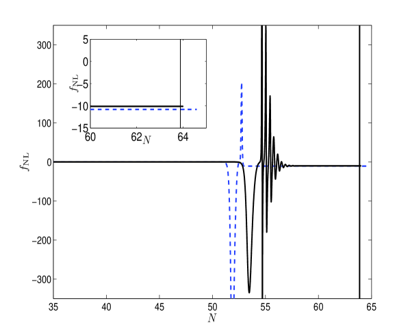
An explicit example is given by $g=(10^{-4}/0.18^{2})m_{\phi}^{2}M_{\rm pl}$, $\lambda=(100/0.18^{2})m_{\phi}^{2}/M_{\rm pl}$ and $r=0.14M_{\rm pl}$, with the value of $m_{\phi}$ implicitly chosen such that the value of $\zeta$ is normalised to be compatible with CMB constraints[22]. Fig. 1 illustrates the evolution of $f_{\mathrm{NL}}$ with the initial condition $\phi^{*}=16M_{\rm pl}$, which supports close to $60$e-folds of inflation, and $\chi^{*}=0.0015M_{\rm pl}$ which represents an initial field position just above the inflection point. The ridge–like shape of the inflection point results in a negative spike in $f_{\mathrm{NL}}$. Subsequently the trajectories converge into a valley, while slow-roll is still maintained, resulting in $f_{\mathrm{NL}}$ temporarily becoming positive before eventually tending to its limiting value. Recalling the discussion of §3, and bearing in mind the initial conditions, we find that $N_{,\chi}=V_{\chi}/V_{\chi}^{\prime}$ is the dominant first derivative of $N$, and moreover $V_{\chi}^{\prime\prime}/V_{\chi}$ is large and positive (since the field is initially above the inflection point). We therefore expect a large negative asymptotic value of $f_{\mathrm{NL}}$, which is borne out by the full numerical evolution. The numerical and HCA limiting values are both shown in Fig. 1, which show excellent agreement, since slow-roll is maintained throughout the evolution. We note that placing the field initially at $\chi^{*}=-0.0015M_{\rm pl}$, where $V_{\chi}^{\prime\prime}$ is negative, leads to nearly identical evolution, except that a positive $f_{\mathrm{NL}}$ is ultimately reached (with the numerically calculated value of $f_{\mathrm{NL}}=9.9$ in good agreement with the analytic HCA value of $f_{\mathrm{NL}}=10.4$). Finally, choosing initial conditions very close to $\chi^{*}=0$, leads to a negligible $f_{\mathrm{NL}}$, which again is expected since $V_{\chi}^{\prime\prime}\sim 0$.

Figure 1: Evolution of $f_{\mathrm{NL}}$ for the potential (15) with parameter values and initial conditions given in the text. The solid line shows the full numerical evolution while the dashed line gives the analytic solution. The thin vertical line at $N\approx 64$ represents the analytically calculated end of inflation when slow roll completely breaks down. The fact that the adiabatic limit value of $f_{\mathrm{NL}}=-10.1$ (seen in the insert) has been reached long before this point explains why the ‘HCA’ analytic value of $f_{\mathrm{NL}}-10.8$ is a good approximation.

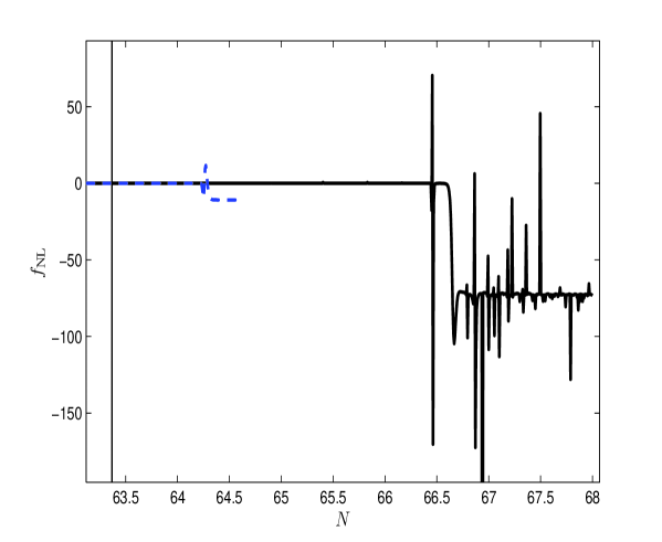
Now let us change the parameters so that instead of reaching the adiabatic limit before inflation ends, it is reached just afterwards. We choose $g=10^{-4}m_{\phi}^{2}M_{\rm pl}$, $\lambda=100m_{\phi}^{2}/M_{\rm pl}$ and $r=0.14M_{\rm pl}$, and the same initial conditions ($\phi^{*}=16M_{\rm pl},\chi^{*}=0.0015M_{\rm pl}$). It is clear that the analytic HCA value for $f_{\mathrm{NL}}$ can no longer be trusted, but one might hope that it gives at least an indication of the true asymptotic value, particularly as the $\chi$ field will source a final fraction of an e-fold of inflation as it rolls. Studying Fig. 2, this is seen not to be the case, with the analytic estimate (unchanged from the above case) being extremely inaccurate.

Figure 2: Evolution of $f_{\mathrm{NL}}$ for the potential (15) with parameters and initial conditions given in the text. As before, the solid line shows the full numerical evolution, the dashed line the slow-roll analytic evolution, and the thin vertical line shows the analytically calculated time when slow-roll breaks down. A discrepancy between the analytic and numerical evolution is not unexpected, though its magnitude is perhaps a surprise.

6 Conclusions

We have studied the evolution of non-Gaussianity in multiple-field inflationary models, using analytical and numerical methods. We have shown that the descent of fields from a ridge or their convergence into a valley can result in significant growth of non-Gaussianity, with the two cases being distinguished by the sign of $f_{\mathrm{NL}}$.

To concretely predict non-Gaussianities one can employ analytical expressions or numerical methods. Currently, however, the former rely on the slow-roll approximation which limits their applicability. In such cases we have demonstrated that numerical methods can be invaluable.

To calculate observationally relevant values of parameters such as $f_{\mathrm{NL}}$, in practice it is necessary that an adiabatic limit is reached where these parameters become constant. In order to determine the possible behaviours of $f_{\mathrm{NL}}$ as it reaches this limit, and the techniques needed to calculate it accurately there, we have found it is useful to classify inflationary models according to whether the adiabatic limit is reached naturally by the convergence of field space trajectories during the slow-roll regime, naturally after slow-roll ends, abruptly, or where no focusing region exists, only after reheating occurs. We have summarised the recent results from our paper[13] concerning these classes of models and given a new illustration here using a new model.

Finally, we note that the new example included in this work indicates that it is easy to construct two-field sum–separable models which exhibit large $f_{\mathrm{NL}}$ of positive or negative sign, even when the adiabatic limit is reached naturally during slow-roll inflation. We note, however, that all such models exhibiting a large non-Gaussianity at the adiabatic limit appear to require a large degree of fine tuning in their initial conditions.

References

- [1] J. M. Bardeen, P. J. Steinhardt, M. S. Turner, Phys. Rev. D 28, 679 (1983); D. H. Lyth, Phys. Rev. D 31, 1792 (1985); D. H. Lyth, K. A. Malik, M. Sasaki, JCAP 0505, 004 (2005); G. I. Rigopoulos, E. P. S. Shellard, Phys. Rev. D 68, 123518 (2003); D. Langlois and F. Vernizzi, Phys. Rev. D 72, 103501 (2005); S. Weinberg, Phys. Rev. D 70, 043541 (2004).
- [2] D. H. Lyth, Phys. Rev. D 31, 1792 (1985).
- [3] J. M. Maldacena, JHEP 0305, 013 (2003).
- [4] J. Garcia-Bellido, D. Wands, Phys. Rev. D 53, 5437 (1996).
- [5] C. Gordon, D. Wands, B. A. Bassett, R. Maartens, Phys. Rev. D 63, 023506 (2001).
- [6] F. Vernizzi and D. Wands, JCAP 0605, 019 (2006).
- [7] G. I. Rigopoulos, E. P. S. Shellard, B. J. W. van Tent, Phys. Rev. D 73, 083521 (2006); G. I. Rigopoulos, E. P. S. Shellard, B. J. W. van Tent, Phys. Rev. D 76, 083512 (2007); S. Yokoyama, T. Suyama and T. Tanaka, JCAP 0707, 013 (2007); S. Yokoyama, T. Suyama and T. Tanaka, Phys. Rev. D 77, 083511 (2008); D. J. Mulryne, D. Seery and D. Wesley, JCAP 1104, 030 (2011); D. J. Mulryne, D. Seery and D. Wesley, JCAP 1001, 024 (2010).
- [8] D. Seery, J. E. Lidsey, JCAP 0509, 011 (2005); D. Seery, J. E. Lidsey and M. S. Sloth, JCAP 0701, 027 (2007); D. Seery, M. S. Sloth and F. Vernizzi, JCAP 0903, 018 (2009).
- [9] L. Alabidi, JCAP 0610, 015 (2006); C. T. Byrnes, K. Y. Choi and L. M. H. Hall, JCAP 0902, 017 (2009).
- [10] C. T. Byrnes, K. Y. Choi and L. M. H. Hall, JCAP 0810, 008 (2008).
- [11] S. A. Kim, A. R. Liddle and D. Seery, Phys. Rev. Lett. 105, 181302 (2010).
- [12] C. M. Peterson and M. Tegmark, ‘Non-Gaussianity in Two-Field Inflation,’ [arXiv:1011.6675 [astro-ph.CO]].
- [13] J. Elliston, D. J. Mulryne, D. Seery and R. Tavakol, ‘Evolution of to the adiabatic limit,’ [arXiv:1106.2153 [astro-ph.CO]].
- [14] A. A. Starobinsky, JETP Lett. 42, 152 (1985).
- [15] M. Sasaki and E. D. Stewart, Prog. Theor. Phys. 95, 71 (1996).
- [16] D. Wands, K. A. Malik, D. H. Lyth and A. R. Liddle, Phys. Rev. D 62, 043527 (2000).
- [17] D. H. Lyth and Y. Rodriguez, Phys. Rev. Lett. 95, 121302 (2005).
- [18] S. W. Hawking, Astrophys. J. 145, 544 (1966); A. A. Starobinsky, Phys. Lett. B 117, 175 (1982); D. S. Salopek, Phys. Rev. D 52, 5563 (1995).
- [19] T. Battefeld and R. Easther, JCAP 0703, 020 (2007).
- [20] K. -Y. Choi, L. M. H. Hall and C. van de Bruck, JCAP 0702, 029 (2007).
- [21] T. Wang, Phys. Rev. D 82, 123515 (2010).
- [22] D. Larson et al., Astrophys. J. Suppl. 192, 16 (2011) [arXiv:1001.4635 [astro-ph.CO]]; E. Komatsu et al. [WMAP Collaboration], Astrophys. J. Suppl. 192, 18 (2011).
- [23] E. Komatsu et al., ‘Non-Gaussianity as a Probe of the Physics of the Primordial Universe and the Astrophysics of the Low Redshift Universe,’ [arXiv:0902.4759 [astro-ph.CO]].
- [24] S. A. Kim, A. R. Liddle, Phys. Rev. D 74, 023513 (2006). S. A. Kim, A. R. Liddle, Phys. Rev. D 74, 063522 (2006).