How genealogies are affected by the speed of evolution

Abstract

In a series of recent works it has been shown that a class of simple models of evolving populations under selection leads to genealogical trees whose statistics are given by the Bolthausen-Sznitman coalescent rather than by the well known Kingman coalescent in the case of neutral evolution. Here we show that when conditioning the genealogies on the speed of evolution, one finds a one parameter family of tree statistics which interpolates between the Bolthausen-Sznitman and Kingman’s coalescents. This interpolation can be calculated explicitly for one specific version of the model, the exponential model. Numerical simulations of another version of the model and a phenomenological theory indicate that this one-parameter family of tree statistics could be universal. We compare this tree structure with those appearing in other contexts, in particular in the mean field theory of spin glasses.

1 Introduction

An important question in the study of evolving populations is to understand the effect of selection on the ancestry and on the genealogies [3, 2, 4, 5, 1]. In absence of selection, for a well mixed population such as in the Wright-Fisher model, the statistical properties of the genealogy of a large population of constant size is described by Kingman’s coalescent [9, 8, 7, 6]. Recent attempts to modify the Wright-Fisher model in order to introduce selection lead to a change of the statistical properties of genealogies: in [10, 11], the study of a whole class of models indicates that the genealogies of populations evolving under selection are given by Bolthausen-Sznitman’s coalescent [12] rather than by Kingman’s (this has been shown analytically only for one specific version of the model, the exponential model (see below), but it has also been checked in numerical simulations and proved for a modified version of the model where the effect of selection is represented by a moving absorbing wall along the fitness axis [13]). In the present paper, we further study these simple models of evolution with selection and we calculate how the statistical properties of the genealogies are correlated to the speed of evolution.

The models of evolution with selection we consider here have been introduced in [10, 11] (see also [15, 14]). They can be defined as follows: at each generation $t$ the population consists of a fixed number $N$ of individuals and each individual $i$ is characterized by a single number $x_{i}(t)$ representing its adaptation in the environment. So $x_{i}(t)$ is the position of individual $i$ on a fitness or adaptation axis (very much like in the Bak-Sneppen model [16]). This individual has several offspring at positions $x_{i}(t)+\epsilon_{i,1}(t)$, $x_{i}(t)+\epsilon_{i,2}(t)$, $x_{i}(t)+\epsilon_{i,3}(t)$, etc., where the $\epsilon_{i,j}(t)$ are random numbers representing the change of adaptation due to mutations between parent $i$ and child $j$. The total number of offspring produced this way by all individuals at a given generation $t$ exceeds $N$; the population at generation $t+1$ is then obtained by keeping the $N$ most adapted children (i.e. the $N$ rightmost points along the axis) among all these offspring, see figure 1. The model is fully specified when the distribution of the number offspring of each individual and the distribution of the random shifts $\epsilon$ are given.

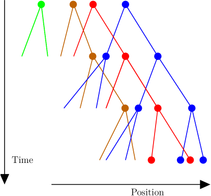
Figure 1: Three time steps for a population of size $N=4$ in a model where each individual has two offspring.

After letting such a model evolve for a large number $t$ of generations, the positions $x_{i}(t)$ of the individuals on the adaptation axis from a cloud of points grouped around a position $X_{t}$ which grows linearly with time with some velocity $v_{N}$. There is some arbitrariness in the way this position $X_{t}$ can be defined (one could choose for example $X_{t}$ to be the position of the rightmost individual, or of the leftmost individual or the center of mass of the population) but, as the positions of all the individuals remain grouped, a change of definition modifies the value of $X_{t}$ by an amount which does not grow with time and therefore does not affect the velocity $v_{N}$. In addition to the velocity, the position $X_{t}$ has fluctuations: in particular it diffuses with a variance which grows linearly in time [17].

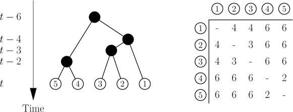
Figure 2: Left: an exemple of the genealogical tree of $N=5$ individuals. Right: the coalescence times $\tau_{i,j}(t)$ corresponding to the tree.

At each generation, one can study the genealogy of the population of this model by considering the matrix $\tau_{i,j}(t)$ of the ages of the most recent common ancestors, or coalescence times, of all pairs of individuals $i$ and $j$ living at generation $t$; see figure 2. As the genealogy is a tree, the whole ancestry of the population can be deduced from the knowledge of this matrix. In particular the age of the most recent common ancestor of any subset of the population can be expressed in terms of this matrix: for example the age $\tau_{i,j,k}(t)$ of the most recent common ancestor of three individuals $i$, $j$ and $k$ at generation $t$ is simply

$$\tau_{i,j,k}(t)=\max\big{(}\tau_{i,j}(t),\tau_{i,k}(t),\tau_{j,k}(t)\big{)}.$$ (1)

One property common to the models of evolution under selection studied here and to the neutral models of evolution described by Kingman’s coalescent is that the heights and the shapes of the genealogical trees fluctuate with $t$ even when the size $N$ of the population becomes large. The statistical properties of these trees and their time scales are however different: for instance, the typical age of the most recent common ancestors of $k$ individuals grows logarithmically with the population size $N$ in presence of selection (as in the models studied here) while it grows linearly with $N$ in the neutral case.

There are several ways of describing the statistical properties of these trees (see section 5). In [10, 11] we chose to characterize them by the average coalescence times $\langle T_{k}\rangle$ of $k$ individuals chosen at random in the population:

$$\langle T_{k}\rangle=\big{\langle}\tau_{i_{1},\ldots,i_{k}}(t)\big{\rangle}.$$ (2)

(here $\langle\cdot\rangle$ denotes an average over the individuals $i_{1},\ldots,i_{k}$ and over the generation $t$). The $N$ dependence of $\langle T_{2}\rangle$ gives the time scale over which coalescence events occur, while the ratios $\langle T_{k}\rangle/\langle T_{2}\rangle$ are a signature of the statistical properties of the shape of the trees. We found in [10, 11] that these ratios in presence of selection converge when $N\to\infty$ to those of a Bolthausen-Snitzmann coalescent:

$$\frac{\langle T_{3}\rangle}{\langle T_{2}\rangle}=\frac{5}{4},\qquad\frac{\langle T_{4}\rangle}{\langle T_{2}\rangle}=\frac{25}{18},$$ (Bolthausen-Snitzmann) (3)

in contrast to the neutral case where they converge to those of Kingman’s coalescent:

$$\frac{\langle T_{3}\rangle}{\langle T_{2}\rangle}=\frac{4}{3},\qquad\frac{\langle T_{4}\rangle}{\langle T_{2}\rangle}=\frac{3}{2}.$$ (Kingman) (4)

Our goal here is to calculate how these ratios are correlated to the speed of evolution, by weighting all the events during a long time interval $\tau$ by a factor $e^{-\beta X_{\tau}}$. ($\beta<0$ favors events with a speed of evolution faster than average, while $\beta>0$ correponds to events with a slower speed of evolution.) Our main result, derived below for the exponential model, is that the above ratios become for large $N$

$$\frac{\langle T_{3}\rangle}{\langle T_{2}\rangle}=\frac{5+4\beta}{4+3\beta},\qquad\frac{\langle T_{4}\rangle}{\langle T_{2}\rangle}=\frac{100+204\beta+133\beta^{2}+27\beta^{3}}{72+142\beta+90\beta^{2}+18\beta^{3}}$$ (5)

It is remarkable that these expressions interpolate between the neutral case (Kingman) for $\beta\to+\infty$ (low speed limit) and the selection case (Bolthausen-Snitzmann) for $\beta=0$. When $\beta\to-1$ (high speed limit), all the ratios become $1$ indicating a “star-shaped” coalescent.

This paper is organized as follows: in section 2, we explain how the weighting by the factor $e^{-\beta X_{\tau}}$ is done. In section 3, we show that in presence of the bias, one version of the model (the exponential model) can be solved exactly by analyzing a coalescent model, the rates of which depend on $\beta$. This leads to (5). In section 4 we argue using the phenomenological theory developed in [11] that (5) should remain valid for other versions of the model up to a change of scale of $\beta$. Lastly in section 5 we compare the $\beta$-random tree structure which leads to (5) to the statistics of the partitions in mean field spin glasses and in the Poisson-Dirichlet distribution.

2 How to condition on the velocity

If one performs a simulation of the model described in the introduction, one can measure at each generation $t$ the position $X_{t}$ of the population (defined in any reasonable way: as explained in the introduction, the precise definition does not matter) and the ages $T_{2}(t),\ldots,T_{k}(t)$ of the most recent common ancestor of $2,\ldots,k$ individuals chosen at random in the population at time $t$ (for more efficiency one can average these times $T_{k}(t)$ over all the choices of the $k$ individuals in the population at time $t$). Then we choose a long time interval $\tau$ and we want to determine

$$\langle T_{k}\rangle_{\beta}=\lim_{\tau\to\infty}\frac{1}{\tau}\sum_{t=1}^{\tau}\frac{\big{\langle}T_{k}(t)e^{-\beta X_{\tau}}\big{\rangle}}{\big{\langle}e^{-\beta X_{\tau}}\big{\rangle}}.$$ (6)

2.1 Theoretical considerations

As the model is a Markov process and correlations decay fast enough in time, we expect that, for large $t$,

$$\left\langle e^{-\beta(X_{t}-X_{0})}\right\rangle\sim e^{tG(\beta)}.$$ (7)

The knowledge of $G(\beta)$ determines all the cumulants of the position $X_{t}$

$$\lim_{t\to\infty}\frac{\langle X_{t}^{n}\rangle_{c}}{t}=(-)^{n}\left.\frac{\text{d}^{n}G(\beta)}{\text{d}\beta^{n}}\right|_{\beta=0}.$$ (8)

It is also related to the large deviation function $F(v)$ of the velocity defined by

$$\text{Proba}(X_{t}=vt)\sim e^{tF(v)}$$ (9)

through a Legendre transform

$$G(\beta)=\max_{v}[-\beta v+F(v)].$$ (10)

For large $t$, the value of $v$ which dominates the weighted averages in (6) and (7) is given by

$$v=-\frac{\text{d}G(\beta)}{\text{d}\beta},$$ (11)

with fluctuations of order $t^{-1/2}$. Therefore the weighted averages (6) become equivalent in the $t\to\infty$ limit to conditioning on the velocity $v$ given by (11). This is, in the present context, the analog of the well known equivalence of ensembles in statistical physics.

2.2 In numerical simulations

Numerically it is difficult to perform averages such as (6) because the events which dominate both the numerator and the denominator of (6) are rare events. In order to overcome this difficulty, we use an importance sampling method. We consider a sample periodic in time of period $\tau$ where $\tau$ is chosen large enough. This means that the random shifts $\epsilon_{i,j}(t)$ are periodic in time ($\epsilon_{i,j}(t+\tau)=\epsilon_{i,j}(t)$ for all $i$, $j$ and $t$). With these periodic $\epsilon_{i,j}(t)$, the evolution of the system becomes also periodic in time: the shift $X_{\tau}$ of the position of the population after one period $\tau$ can therefore be unambigously defined and depends on all the $\epsilon_{i,j}(t)$. Then, we perform a standard Monte-Carlo simulation: at each step we try a new sample by changing some of the $\epsilon_{i,j}(t)$ and we let the system evolve till it becomes periodic (here we change all the $\epsilon_{i,j}(t)$ at a random time $t$ uniformly distributed between $1$ and $\tau$). The outcome of this change is to modify the $X_{\tau}$ to a new value $X_{\tau}^{\text{new}}$. Then, as always with a Metropolis algorithm, we accept the change with a probability $\max\big{[}1,\exp[-\beta(X_{\tau}^{\text{new}}-X_{\tau})]\big{]}$. With this procedure samples are produced with a weight $\exp[{-\beta X_{\tau}}]$, so that by averaging quantities such as the $T_{k}$ over many samples one gets an estimate of (6).

We have simulated the exponential model (see section 3 where we give the precise definition of the exponential model and its analytic solution in the $N\to\infty$ limit) for $N=100$ and a value of $\tau\approx 30\ln N$ which is much larger than $\langle T_{2}\rangle$ [11]. For each value of $\beta$, we measured $\langle T_{2}\rangle$, $\langle T_{3}\rangle$, $\langle T_{4}\rangle$ averaged on $10^{6}$ Monte-Carlo steps. We have also simulated a more generic model where each individual has exactly two offspring with independent random shifts $\epsilon_{i,j}(t)$ uniformly distributed between 0 and 1. This model cannot be solved exactly, but a phenomenological theory (see [11] and section 4) predicts when $N\to\infty$ the same statistics of the genealogical trees (5) as in the exponential model with $\beta$ replaced by $\beta/\gamma$, where $\gamma\simeq 5.262$ is the value which minimizes the function $\ln[2(e^{\gamma}-1)/\gamma]/\gamma$, see section 4. We simulated the sizes $N=30$, $N=100$ and $N=300$ with values of $\tau\approx 8\ln^{3}N$ which is much larger than $\langle T_{2}\rangle$, and again averaged over $10^{6}$ Monte-Carlo steps. We also checked for several values of $\beta$ that our results remain unchanged by choosing a value of the period $\tau$ twice as big (results not shown), indicating that our Monte-Carlo results would be the same for an infinite time-window.

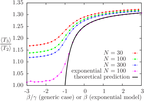
Figure 3: $\langle T_{3}\rangle/\langle T_{2}\rangle$ as a function of $\beta$ for the exponential model and the prediction (5), and as a function of $\beta/\gamma$ for the generic model described in the text.

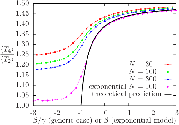
Figure 4: $\langle T_{4}\rangle/\langle T_{2}\rangle$ as a function of $\beta$ for the exponential model and the prediction (5), and as a function of $\beta/\gamma$ for the generic model described in the text.

The results for $\langle T_{3}\rangle/\langle T_{2}\rangle$ and $\langle T_{4}\rangle/\langle T_{2}\rangle$ are presented in figures 3 and 4. As in [11], we observe that for the exponential model, the results are already very close to their asymptotic limits even for $N=100$; only for $\beta\lesssim-1$ there is a discrepancy with the theoretical prediction (5). As in [11], the convergence is however slower in the generic case but the curves seem in both cases to converge to the prediction.

3 Exponential model

In this section we consider a version of the model, the exponential model, which can be solved exactly [11]. In the exponential model, the shifts of the offspring of each individual are generated by a Poisson process of density $\rho(\epsilon)=e^{-\epsilon}$. This means that an individual at position $x_{i}(t)$ has a probability $e^{-\epsilon}\text{d}\epsilon$ of having an offspring in the infinitesimal interval $(x_{i}(t)+\epsilon,x_{i}(t)+\epsilon+\text{d}\epsilon)$. Then the population at the next generation is obtained by selecting the $N$ rightmost points among all the offspring produced by generation $t$. (Note that in the exponential model the number of offspring produced by each generation is infinite but their number at the right of any position $y$ is finite. There is therefore no problem to select the $N$ survivors at generation $t+1$).

In the exponential model, there is a convenient way of defining the position $X_{t}$ of the population

$$X_{t}=\ln\bigg{[}\sum_{i=1}^{N}e^{x_{i}(t)}\bigg{]}.$$ (12)

The simplicity of the exponential model comes from the fact that, with this definition of $X_{t}$, one has

$$\sum_{i}e^{-[x-x_{i}(t)]}=e^{-(x-X_{t})},$$ (13)

which means that one can generate the offspring of the whole population at time $t$ by replacing the $N$ Poisson processes centered at the positions $x_{i}(t)$ by a single Poisson process centered at position $X_{t}$. Therefore, with definition (12) of $X_{t}$, the $N$ points $x_{i}(t+1)$ at generation $t+1$ are the $N$ rightmost points of a Poisson point process with a density $\exp[{-(x-X_{t})}]$.

As explained in [11] a way of drawing these $N$ points is to choose a number $z$ with a density of probability $\text{Proba}(z)=\exp[-(N+1)z-e^{-z}]/N!$ and, independently, $N$ numbers $y_{i}$ with an exponential density $\text{Proba}(y)=e^{-y}\theta(y)$; the points $x_{i}(t+1)$ are then given (in an arbitrary order) by

$$x_{i}(t+1)=X_{t}+z+y_{i},$$ (14)

and one gets from (12)

$$X_{t+1}=X_{t}+z+\ln\bigg{[}\sum_{i=1}^{N}e^{y_{i}}\bigg{]}.$$ (15)

We see that, with the definition (12) of $X_{t}$, the differences $X_{t+1}-X_{t}$ are independent variables. Therefore from (7)

$$e^{tG(\beta)}=\left\langle e^{-\beta(X_{t}-X_{0})}\right\rangle=\left\langle e^{-\beta(X_{t+1}-X_{t})}\right\rangle^{t},$$ (16)

and $G(\beta)$ can be computed by averaging over a single generation

$$e^{G(\beta)} =\langle e^{-\beta z}\rangle\bigg{\langle}\bigg{[}\sum_{i=1}^{N}e^{y_{i}}\bigg{]}^{-\beta}\bigg{\rangle}$$ (17)

$$=\frac{\Gamma(N+1+\beta)}{\Gamma(N+1)}\int_{0}^{\infty}\text{d}y_{1}\cdots\int_{0}^{\infty}\text{d}y_{n}\ e^{-y_{1}-\cdots-y_{N}}\bigg{[}\sum_{i=1}^{N}e^{y_{i}}\bigg{]}^{-\beta}.$$

Using the integral representation (valid for $\beta>0$)

$$A^{-\beta}=\frac{1}{\Gamma(\beta)}\int_{0}^{\infty}\text{d}\lambda\,\lambda^{\beta-1}e^{-\lambda A}\qquad\text{(for $\beta>0$),}$$ (18)

one obtains

$$e^{G(\beta)}=\frac{\Gamma(N+1+\beta)}{\Gamma(N+1)\Gamma(\beta)}\int_{0}^{\infty}\text{d}\lambda\,\lambda^{\beta-1}I_{0}(\lambda)^{N},$$ (19)

where the integral $I_{0}(\lambda)$ and more general integrals $I_{p}(\lambda)$ are defined as

$$I_{p}(\lambda)=\int_{0}^{\infty}\text{d}y\,e^{(p-1)y-\lambda e^{y}}=\lambda^{1-p}\int_{\lambda}^{\infty}\text{d}u\,u^{p-2}e^{-u}.$$ (20)

(These integrals are in fact, up to a simple change of variables, incomplete gamma functions). For large $N$, the expression (19) is dominated by small values of $\lambda$ where the integrals $I_{p}(\lambda)$ for non-negative integers $p$ can be approximated by [11]:

$$\begin{gathered}I_{0}(\lambda)=1+\lambda(\ln\lambda+\gamma_{E}-1)+{\cal O}(\lambda^{2}),\qquad I_{1}(\lambda)=-(\ln\lambda+\gamma_{E})+{\cal O}(\lambda),\\ I_{p\geq 2}(\lambda)={(p-2)!\over\lambda^{p-1}}+{\cal O}(\lambda^{2-p}),\end{gathered}$$ (21)

where $\gamma_{E}=-\Gamma^{\prime}(1)\simeq.577$ is Euler’s constant.

Given the small $\lambda$ expansion of $I_{0}(\lambda)$, the integral in (19) is dominated, for $N$ large and $\beta$ of order 1, by $\lambda$ of order $1/(N\ln N)$. Making the change of variable $\lambda=\mu/(N\ln N)$ one has

$$I_{0}(\lambda)^{N}=e^{-\mu}\left(1+\mu{\ln\mu-\ln\ln N+\gamma_{E}-1\over\ln N}+{\cal O}\Big{(}\frac{\mu\ln\mu}{\ln N}\Big{)}^{2}\right),$$ (22)

We can now evaluate (19) for $N$ large and $\beta$ of order 1; using (22) and $\Gamma(N+1+\beta)/\Gamma(N+1)\simeq N^{\beta}$, one gets [11]

$$e^{G(\beta)}=\frac{1}{\ln^{\beta}N}\left[1+\frac{\beta}{\ln N}\left({\Gamma^{\prime}(\beta+1)\over\Gamma(\beta+1)}-\ln\ln N+\gamma_{E}-1\right)+\cdots\right]$$ (23)

or

$$G(\beta)=-\beta\ln\ln N+\frac{\beta}{\ln N}\left({\Gamma^{\prime}(\beta+1)\over\Gamma(\beta+1)}-\ln\ln N+\gamma_{E}-1\right)+\cdots$$ (24)

We see that, as $v=-G^{\prime}(\beta)$, see (11), varying $\beta$ does not change the leading $N$ dependence $v\simeq\ln\ln N$ of the velocity but only shifts it by a small amount of order $\ln\ln N/\ln N$ which vanishes in the $N\to\infty$ limit. We are now going to show that, on the contrary, $\beta$ does change the statistical properties of the trees even in the $N\to\infty$ limit.

3.1 Trees

We have already seen that all the offspring produced by generation $t$ are distributed according to a Poisson point process of density $\exp[{-(x-X_{t})}]$. On the other hand, the offspring of individual $x_{i}(t)$ are distributed as a Poisson point process of density $\exp\big{[}{-[x-x_{i}(t)]}\big{]}$. This implies that, given that there is an offspring in an interval $\text{d}x$ around $x$, its probability of being an offspring of $x_{i}(t)$ is

$$W_{i}=e^{x_{i}(t)-X_{t}}=\frac{e^{x_{i}(t)}}{\sum_{j=1}^{N}e^{x_{j}(t)}}.$$ (25)

This probability is independent of $x$. Therefore the probability $Q_{p}(t)$ that $p$ individuals at generation $t+1$ have the same ancestor at generation $t$ is

$$Q_{p}(t)=\sum_{i=1}^{N}W_{i}^{p}=\sum_{i=1}^{N}e^{px_{i}(t)-pX_{t}}.$$ (26)

If one weights these coalescence rates with the factor $e^{-\beta X_{t}}$, then using (14) and (15) with $t$ replaced by $t-1$ and using the fact that $X_{t-1}$, $z$ and the $y_{i}$ are independent, one gets

$$\langle Q_{p}\rangle_{\beta}=N\frac{\big{\langle}e^{px_{1}(t)-(\beta+p)X_{t}}\big{\rangle}}{\big{\langle}e^{-\beta X_{t}}\big{\rangle}}=N\frac{\Big{\langle}e^{py_{1}-(\beta+p)\ln\big{[}\sum_{i=1}^{N}e^{y_{i}}\big{]}}\Big{\rangle}}{\Big{\langle}e^{-\beta\ln\big{[}\sum_{i=1}^{N}e^{y_{i}}\big{]}}\Big{\rangle}}$$ (27)

with the $y_{i}$ independent exponential variables. The numerator and the denominator can be computed in the same way as in (19) and one obtains

$$\langle Q_{p}\rangle_{\beta}=N\frac{\Gamma(\beta)}{\Gamma(\beta+p)}\times\frac{\int_{0}^{\infty}\text{d}\lambda\,\lambda^{\beta+p-1}I_{p}(\lambda)I_{0}(\lambda)^{N-1}}{\int_{0}^{\infty}\text{d}\lambda\,\lambda^{\beta-1}I_{0}(\lambda)^{N}}.$$ (28)

We take $p\geq 2$ and $\beta$ of order 1. The integrals are dominated by $\lambda=\mu/(N\ln N)$ and $\mu$ of order 1. To the leading order, $I_{0}(\lambda)^{N}\approx e^{-\mu}$, see (22), and using (21) for $I_{p}(\lambda)$ one easily gets, to leading order

$$\langle Q_{p}\rangle_{\beta}\simeq\frac{1}{\ln N}\,\frac{(p-2)!\,\Gamma(\beta+1)}{\Gamma(\beta+p)}=\frac{1}{\ln N}\,\frac{(p-2)!}{(1+\beta)(2+\beta)\cdots(p-1+\beta)}.$$ (29)

After rescaling time by a factor $\ln N$, one gets a coalescent with transition rates $q_{p}=\langle Q_{p}\rangle_{\beta}\ln N$. One can check that

$$q_{p}=\frac{(p-2)!\,\Gamma(\beta+1)}{\Gamma(\beta+p)}=\int_{0}^{1}x^{p-2}\Lambda(\text{d}x)\qquad\text{with }\Lambda(\text{d}x)=(1-x)^{\beta}\,\text{d}x,$$ (30)

Using the expressions (55) of the appendix, where the ratios ${\langle T_{3}\rangle/\langle T_{2}\rangle}$ and ${\langle T_{4}\rangle/\langle T_{2}\rangle}$ have been obtained for a general coalescent, one finally gets (5).

4 The phenomenological theory

In this section, we show that the phenomenological theory developed in [17, 11] in the context of the noisy Fisher-KPP equation predicts that (5) remains valid for other versions of the model described in the introduction. When the number of offspring of each individual is bounded and when the shifts $\epsilon_{i,j}$ are also bounded, one can describe the evolution of the population by a noisy traveling wave equation of the Fisher-KPP type. In [17, 11], a phenomenological theory was proposed to describe the large $N$ behavior of these noisy equations. In the $N\to\infty$ limit, the effect of noise vanishes and the traveling wave has a finite velocity $v_{\infty}$ (in contrast to the exponential model where the velocity diverges as $N\to\infty$). The first correction when $N$ is large can be understood by considering the cutoff introduced by the discrete number of particles: this leads to $v_{\text{cutoff}}=v_{\infty}-A/\ln^{2}N$. The next order correction leads to a positive term of order $\ln\ln N/\ln^{3}N$ which can be understood, as well as the fluctuations of $X_{t}$, by the following phenomenological theory: the front has, most of the time, the shape and the velocity predicted by the cutoff theory. However, every (typically) $\ln^{3}N$ time steps, a rare event occurs where some particles escape significantly ahead of the front. When this happens, the shape of the front is at first deformed, but it relaxes to its cutoff shape after $\sim\ln^{2}N$ time steps. The end result is a finite increase of the position of the front [11]. It has been shown that this phenomenological theory predicts genealogies described by the Bolthausen-Snitzmann coalescent. We are now going to show that when we condition on the velocity by using the weight $\exp(-\beta X_{t})$, this leads to (5).

We consider a time interval $\Delta t$ which is large compared to $\ln^{2}N$ but small compared to $\ln^{3}N$. During this interval, there is a small probability $p(\delta)\,\text{d}\delta\,\Delta t$ that an event of size $\delta$ occurs. When this happens, the front position increases (after relaxation) by $R(\delta)$. The time interval $\ln^{2}N\ll\Delta t\ll\ln^{3}N$ is such that each event has the time to relax during $\Delta t$ and that the probability that two events occur during the same time interval is negligible.

With these notations, the position $X_{t}$ of the front evolves according to

$$X_{t+\Delta t}-X_{t}=\begin{cases}v_{\text{cutoff}}\Delta t+R(\delta)&\text{proba. }p(\delta)\,\text{d}\delta\,\Delta t,\\ v_{\text{cutoff}}\Delta t+0&\text{proba. }1-\Delta t\int\text{d}\delta\,p(\delta).\end{cases}$$ (31)

We argued in [11] that, for large $\delta$,

$$p(\delta)\approx C_{1}e^{-\gamma\delta},\quad R(\delta)\approx\frac{1}{\gamma}\ln\left(1+C_{2}\frac{\gamma^{3}e^{\gamma\delta}}{\ln^{3}N}\right),\quad C_{1}C_{2}\approx\pi^{2}\gamma v^{\prime\prime}(\gamma).$$ (32)

The number $\gamma$ and the function $v(r)$ depend on the details of the model. (For $N\to\infty$, $v(r)$ gives the velocity of a front starting with the initial condition $e^{-rx}$. For a step initial condition, the system moves at the velocity $v(\gamma)$ where $\gamma$ is the value at which $v(r)$ reaches its minimum.)

Using (31) to compute $G(\beta)$ given by (7), one gets

$$G(\beta)=-\beta v_{\text{cutoff}}+\int\text{d}\delta\,p(\delta)\left[e^{-\beta R(\delta)}-1\right].$$ (33)

Let us now weight all the events by the factor $\exp(-\beta X_{t})$. (31) becomes

$$X_{t+\Delta t}-X_{t}=\begin{cases}v_{\text{cutoff}}\Delta t+R(\delta)&\text{proba. }\frac{1}{Z(\beta)}e^{-\beta[v_{\text{cutoff}}\Delta t+R(\delta)]}p(\delta)\,\text{d}\delta\,\Delta t,\\ v_{\text{cutoff}}\Delta t+0&\text{proba. }\frac{1}{Z(\beta)}e^{-\beta v_{\text{cutoff}}\Delta t}\big{[}1-\Delta t\int\text{d}\delta\,p(\delta)\big{]}.\end{cases}$$ (34)

$Z(\beta)$ is such that the probabilities are normalized; clearly $Z(\beta)=e^{\Delta tG(\beta)}$.

Now, we can try to determine the probability $Q_{p}\,\Delta t$ that the $p$ particles coalesce into one during the time interval $\Delta t$. We argued in [11] that when a rare event of size $\delta$ occurs, a fraction $f=1-e^{-\gamma R(\delta)}$ of the population is replaced by the offspring of the single particle that originated the event ($\gamma$ is the model specific number appearing in (32)). When this happens, there is a probability $f^{p}$ that the $p$ particles coalesce during that interval of time $\Delta t$. This leads to

$$Q_{p}=\int\text{d}\delta\,p(\delta)e^{-\beta R(\delta)}\Big{[}1-e^{-\gamma R(\delta)}\Big{]}^{p}$$ (35)

We can now use (32) in (35). Rewriting the integral in term of the variable $f=1-e^{-\gamma R(\delta)}$ (the fraction of the population replaced by the offspring of an individual), one gets $p(\delta)\,\text{d}\delta=C_{1}C_{2}\gamma^{2}/\ln^{3}N\,\text{d}f/f^{2}$, so that

$$Q_{p}=\frac{C_{1}C_{2}\gamma^{2}}{\ln^{3}N}\int_{0}^{1}f^{p-2}(1-f)^{\beta/\gamma}\,\text{d}f,$$ (36)

which is the same as (30) up to a prefactor (which only changes the time scale) and the fact that $\beta$ is replace by $\beta/\gamma$. Therefore the phenomenological theory leads to the same coalescent as in the exponential model but with a different time scale of order $\ln^{3}N$ instead of $\ln N$.

5 Comparison with mean-field spin glasses and the Poisson-Dirichlet distribution

5.1 Various ways of characterizing random trees

There are several ways of characterizing the statistical properties of the trees generated by some given coalescence rates. (We only consider here the cases where the coalescence rates do not vary in time, where the particles play symmetrical roles and where at most one coalescence event can occur during an interval of time $\text{d}t$.)

• One can specify the coalescence rates $q_{p}$ (which take the values (30) for the models of evolution with selection that we consider in this paper). In terms of these coalescence rates, Kingman’s coalescent corresponds to

  $$q_{2}\neq 0,\qquad q_{p}=0\quad\text{for}\ p\geq 3,$$ (37)

  while the Bolthausen-Sznitman coalescent corresponds to

  $$q_{p}={q_{2}\over p-1}.$$ (38)

  It is easy to see that the rates (30) interpolate between (37) for $\beta=\infty$ and (38) for $\beta=0$.

• One can alternatively specify all the ratios ${\langle T_{p}\rangle/\langle T_{2}\rangle}$ . It is clear (see (52,55) in the appendix) that the knowledge of the $q_{p}$ determines all these time ratios and conversely that the knowledge of the time ratios allows one to calculate all the ratios $q_{p}/q_{2}$.

• One can also characterize the trees by the partition of the population they induce at a given time in the past: the population at a generation $t$ can be decomposed into several $\tau$-families where, by definition of these families, two individuals $i$ and $j$ belong to the same $\tau$-family if the age of their most recent common ancestor is less than $\tau$ (i.e. $\tau_{i,j}(t)<\tau$). One can then associate to this $\tau$-partition of the population at generation $t$ the following numbers

  $$Y_{k}^{(\tau)}(t)=\big{\langle}\theta(\tau-\tau_{i_{1},\ldots,i_{k}})\big{\rangle}_{t}$$ (39)

  where $\langle\cdot\rangle_{t}$ means an average over all the possible choices of the $k$ individuals $i_{1},\ldots,i_{k}$ at generation $t$.

  One can interpret these $Y_{k}^{(\tau)}(t)$ as the probability that $k$ individuals chosen at random in the population at generation $t$ belong to the same $\tau$-family. These $Y_{k}^{(\tau)}(t)$ fluctuate from generation to generation and the expressions $\langle Y_{k}^{(\tau)}\rangle$ of their averages over $t$ can be computed in terms of the coalescence rates $q_{p}$. In the appendix, they are given for $k=2,3,4$ by the quantities $Z_{k\to 1}(\tau)\equiv\langle Y_{k}^{(\tau)}\rangle$.

  Knowing all the $\langle Y_{k}^{(\tau)}\rangle$ (even for a single $\tau$) determines also in principle all the coalescence rates and therefore all the statistical properties of the trees.

5.2 Comparison with mean-field spin glasses

Very much like in the coalescence problems discussed above, where all the individuals at a generation $t$ can be grouped into $\tau$-families, one can group the spin configurations of a spin glass model according to their distances $d$ (or to their overlap$=1-d$) in phase space. One can then define [18], for a given sample, the probability $Y_{k}(d)$ that $k$ configurations, at thermal equilibrium, have all their $k(k-1)/2$ mutual distances in phase space less than $d$.

One of the predictions [18, 20, 19] of the Parisi solution [23, 21, 22] of the Sherrington Kirkpatrick model [25, 24] is that this $Y_{k}(d)$ fluctuates with the spin glass sample even when the system size becomes large. The Parisi theory predicts also all the statistical properties of these $Y_{k}(d)$. For example

$$\langle Y_{k}(d)\rangle=\lim_{n\to 0}y_{k}(n,\mu)={\Gamma(k-\mu)\over\Gamma(k)\ \Gamma(1-\mu)}$$ (40)

where according to the broken replica symmetry

$$y_{k}(n,\mu)={\Gamma(1-n)\ \Gamma(k-\mu)\over\Gamma(k-n)\ \Gamma(1-\mu)}.$$ (41)

In (40) all the dependence on the distance $d$, on the details of the model, and on the parameters such as the temperature or the magnetic field is through the parameter $\mu$. Formula (41) follows from a very simple replica calculation: assume that one has $n$ replicas grouped into ${n/\mu}$ families of $\mu$ replicas, $y_{k}(n,\mu)$ is simply the probability that $k$ replicas chosen at random among the $n$ replicas belong to the same family.

For typical samples one has to take the $n\to 0$ limit as in (40) and the statistics of the $Y_{k}$ coincide with those of the Bolthausen-Sznitman coalescent: one can check that the $Z_{k\to 1}(\tau)\equiv\langle Y_{k}^{(\tau)}\rangle$ obtained in (57) coincides with (40) by choosing $\mu=e^{-q_{2}\tau}$ and the $q_{p}$ given by (38).

In the spin glass case, one can also weight the samples according to their free energy (by weighting them by a factor $Z^{n}$ where $Z$ is the partition function [27, 26]). One then expects from the replica theory [26] that the statistics of the $Y_{k}(d)$ be modified and that

$$\frac{\langle Z^{n}\ Y_{k}(d)\rangle}{\langle Z^{n}\rangle}=y_{k}(n,\mu).$$ (42)

One can check easily from (57) with $q_{p}$ given by (30) that there exists no choice of $n$ and $\mu$ as functions of $\beta$ and $\tau$ such that $y_{k}(n,\mu)=Z_{k\to 1}(\tau)$. Therefore, although the statistical properties of the trees in the model of evolution with selection and in the spin glass problem are the same for typical samples, they become different when one introduces a bias (related to the free energy in the spin glass problem and to the speed of adaptation in the models of evolution with selection).

5.3 The Poisson-Dirichlet distribution

The Poisson-Dirichlet distribution [29, 28] is a probability distribution of the partitions of a unit interval into infinitely many subintervals. It is parametrized by two parameters $\alpha$ and $\theta$. One way of defining the Poisson-Dirichlet distribution is to consider an infinite sequence $z_{1}$, $z_{2}$, …, $z_{n}$, …of independent numbers, each $z_{n}$ being distributed according to a distribution

$$P_{n}(z_{n})=\frac{\Gamma(1+\theta+n\alpha-\alpha)}{\Gamma(1-\alpha)\Gamma(\theta+n\alpha)}z_{n}^{-\alpha}(1-z_{n})^{\theta+n\alpha-1}$$ (43)

(which is a $\beta$ distribution). Then one considers a partition of the unit interval into subintervals of lengths $W_{1}$, $W_{2}$, …$W_{n}$, …with

$$W_{1}+W_{2}+\cdots+W_{n}+\cdots=1,$$ (44)

where the $W_{i}$ are given by

$$W_{1}=z_{1},$$ (45)

$$W_{2}=(1-z_{1})z_{2},$$

$$\ldots$$

$$W_{n}=(1-z_{1})(1-z_{2})\cdots(1-z_{n-1})z_{n},$$

$$\ldots$$

For such a partition one can introduce the quantities

$$Y_{k}=\sum_{i}W_{i}^{k},$$ (46)

which represents the probability that $k$ points chosen at random on the unit interval fall in the same subinterval. It is easy to check that when one averages over the $z_{i}$, one gets

$$\langle Y_{k}\rangle_{\alpha,\theta}=\big{\langle}z_{1}^{k}\big{\rangle}+\big{\langle}(1-z_{1})^{k}\big{\rangle}\langle Y_{k}\rangle_{\alpha,\alpha+\theta},$$ (47)

The solution of this recursion is

$$\langle Y_{k}\rangle_{\alpha,\theta}=\frac{\Gamma(1+\theta)\Gamma(k-\alpha)}{\Gamma(k+\theta)\Gamma(1-\alpha)}.$$ (48)

One can notice [30] that these expressions are identical to the replica expressions (41) of $y_{k}(n,\mu)$ when one chooses $\theta=-n$ and $\alpha=\mu$. Therefore as soon as one introduces the bias $\beta\neq 0$ the statistical properties $\tau$-families of our models of evolution with selection differ from those of the Poisson-Dirichlet distribution.

6 Conclusion

In this paper we have seen that, for a family of simple models of evolution under selection, the statistics of the genalogies are modified when conditioning on the speed of evolution (5). For one particular version of these models, the exponential model, the trees can be generated by a coalescent with modified rates (30). Numerical simulations (figures 3 and 4) and a phenomenological theory (section 4) indicate a similar behavior of more generic versions of the model.

Despite their simplicity, there is not yet a full theoretical understanding of the models of evolution with selection we consider here. The introduction of the bias opens new questions which would be interesting to consider. For exemple, what is the effect of the bias on the steady state density profile of the population along the fitness axis, or on the distances between the rightmost points in the population? Numerically, the Monte-Carlo approach we developed here should give a rather powerful tool to study these questions accurately and to test more precisely the phenomenological theory developped in [17, 11].

It would also be interesting to study the genealogies of other models of evolution with selection[31] to test the genericity of our results.

We are very happy to dedicate this work to David Sherrington, on the occasion of his $70^{\rm th}$ birthday.

Appendix A Coalescence times and sizes of families in the $\Lambda$ coalescent

In this appendix we calculate a few simple properties of a continuous time coalescent defined as follows: one starts with $N$ points and during every infinitesimal time interval $\text{d}t\ll 1$, every subset of $k$ points has a probability $q_{k}\,\text{d}t$ of coalescing into one point. It is assumed that there is at most one coalescence event during a time interval $\text{d}t$.

This model is called the $\Lambda$-coalescent [33, 32, 34, 13, 28]. The coalescence rates can be written [33] in terms of a positive measure $\Lambda$ on the interval $(0,1)$

$$q_{k}=\int_{0}^{1}x^{k-2}\Lambda(\text{d}x),$$ (49)

and, more generally [33], the rate $\lambda_{b,k}$ at which the $k\geq 2$ first points out of $b$ coalesce into one point (while the other $b-k$ points remain single) is given by

$$\lambda_{b,k}=\int_{0}^{1}x^{k-2}(1-x)^{b-k}\,\Lambda(\text{d}x)=\sum_{n=0}^{b-k}\frac{(b-k)!}{n!(b-k-n)!}(-1)^{n}q_{n+k}.$$ (50)

It is more convenient in the following to use of the quantities $r_{b}(b^{\prime})$, defined as the rate at which a set of $b$ points coalesce into a set of $b^{\prime}<b$ points. Clearly

$$r_{b}(b^{\prime})=\frac{b!}{(b^{\prime}-1)!(b-b^{\prime}+1)!}\lambda_{b,b-b^{\prime}+1}$$ (51)

(This simply means that the total number of distinct points jumps from $b$ to $b^{\prime}$ with probability $r_{b}(b^{\prime})\text{d}t$ during an infinitesimal time interval $\text{d}t$. The binomial factor in (51) comes from the number of ways of choosing the $b-b^{\prime}+1$ points which coalesce.)

As already noticed, the rates (30) correspond to $\Lambda(\text{d}x)=(1-x)^{\beta}\text{d}x$.

By analyzing what happens during a time interval $\text{d}t$ one can then see that the age $T_{b}$ of the most recent common ancestor of $b$ individuals chosen at generation $t+\text{d}t$ satisfies

$$T_{b}(t+\text{d}t)=\left\{\begin{array}[]{lll}\text{d}t&{\rm with\ probability}&r_{b}(1)\,\text{d}t,\\ \text{d}t+T_{2}(t)&&r_{b}(2)\,\text{d}t,\\ \ldots&&\\ \text{d}t+T_{b-1}(t)&&r_{b}(b-1)\,\text{d}t,\\ \text{d}t+T_{b}(t)&&1-\sum_{b^{\prime}=1}^{b-1}r_{b}(b^{\prime})\,\text{d}t.\end{array}\right.$$ (52)

Therefore one can determine recursively the average coalescence times by writing that $\langle T_{b}(t+\text{d}t)\rangle=\langle T_{b}(t)\rangle$, which leads to

$$\left[\sum_{b^{\prime}=1}^{b-1}r_{b}(b^{\prime})\right]\langle{T_{b}}\rangle=1+\sum_{b^{\prime}=2}^{b-1}r_{b}(b^{\prime})\langle T_{b^{\prime}}\rangle$$ (53)

As (50, 51) imply that

$$r_{2}(1) =q_{2},$$ (54)

$$r_{3}(1) =q_{3},\quad r_{3}(2) =3(q_{2}-q_{3}),$$

$$r_{4}(1) =q_{4},\quad r_{4}(2) =4(q_{3}-q_{4}),\quad r_{4}(3) =6(q_{2}-2q_{3}+q_{4}),$$

one gets

$$\langle T_{2}\rangle =\frac{1}{q_{2}},\qquad\qquad\frac{\langle T_{3}\rangle}{\langle T_{2}\rangle}=\frac{4q_{2}-3q_{3}}{3q_{2}-2q_{3}},$$ (55)

$$\frac{\langle T_{4}\rangle}{\langle T_{2}\rangle} =\frac{27q_{2}^{2}-56q_{2}q_{3}+28q_{3}^{2}+12q_{2}q_{4}-10q_{3}q_{4}}{(3q_{2}-2q_{3})(6q_{2}-8q_{3}+3q_{4})}.$$

If one defines $Z_{b\to b^{\prime}}(\tau)$ as the probability that $b$ points have coalesced into $b^{\prime}$ points during some time $\tau$, one can easily see that it evolves according to

$$\frac{\text{d}Z_{b\to b^{\prime}}}{\text{d}\tau}=\sum_{b^{\prime\prime}>b^{\prime}}r_{b^{\prime\prime}}(b^{\prime})\ Z_{b\to b^{\prime\prime}}\ -\sum_{b^{\prime\prime}<b^{\prime}}r_{b^{\prime}}(b^{\prime\prime})\ Z_{b\to b^{\prime}},$$ (56)

with the initial condition that $Z_{b\to b^{\prime}}(0)=\delta_{b,b^{\prime}}$. Then, using the expressions (54) one gets

$$Z_{2\to 2}=e^{-q_{2}\tau},$$

$$Z_{2\to 1}=1-e^{-q_{2}\tau},$$

$$Z_{3\to 3}=e^{-(3q_{2}-2q_{3})\tau},$$

$$Z_{3\to 2}={3\over 2}e^{-q_{2}\tau}-{3\over 2}e^{-(3q_{2}-2q_{3})\tau},$$

$$Z_{3\to 1}=1-{3\over 2}e^{-q_{2}\tau}+{1\over 2}e^{-(3q_{2}-2q_{3})\tau},$$ (57)

$$Z_{4\to 4}=e^{-(6q_{2}-8q_{3}+3q_{4})\tau},$$

$$Z_{4\to 3}=2e^{-(3q_{2}-2q_{3})\tau}-2e^{-(6q_{2}-8q_{3}+3q_{4})\tau},$$

$$Z_{4\to 2}={9q_{2}-14q_{3}+5q_{4}\over 5q_{2}-8q_{3}+3q_{4}}e^{-q_{2}\tau}-2e^{-(3q_{2}-2q_{3})\tau}+{6q_{2}-10q_{3}+4q_{4}\over 5q_{2}-8q_{3}+3q_{4}}e^{-(6q_{2}-8q_{3}+3q_{4})\tau},$$

$$Z_{4\to 1}=1-{9q_{2}-14q_{3}+5q_{4}\over 5q_{2}-8q_{3}+3q_{4}}e^{-q_{2}\tau}+e^{-(3q_{2}-2q_{3})\tau}-{q_{2}-2q_{3}+q_{4}\over 5q_{2}-8q_{3}+3q_{4}}e^{-(6q_{2}-8q_{3}+3q_{4})\tau}.$$

References

- [1] J. Degnan and L. Salter, Evolution 59 (2005) p.24–37.
- [2] R.R. Hudson, Oxford Surveys in Evolutionary Biology 7 (1991) p.1–44.
- [3] R.R. Hudson and N.L. Kaplan, Genetics 120 (1988) p.831–840.
- [4] C. Neuhauser and S. Krone, Genetics 145 (1997) p.519–534.
- [5] M. Nordborg, Handbook of Statistical Genetics (2001) p.179–212.
- [6] B. Derrida and L. Peliti, Bull. Math. Biol. 53 (1991) p.355–382.
- [7] P. Donnelly and S. Tavare, Annual Review of Genetics 29 (1995) p.401–421.
- [8] J.F.C. Kingman, Stoch. Proc. Appl. 13 (1982) p.235–248.
- [9] J.F.C. Kingman, J. Appl. Probab. 19 (1982) p.27–43.
- [10] É. Brunet, B. Derrida, A.H. Mueller and S. Munier, Europhys. Lett. 76 (2006) p.1–7.
- [11] É. Brunet, B. Derrida, A.H. Mueller and S. Munier, Phys. Rev. E 76 (2007) p.041104.
- [12] E. Bolthausen and A.S. Sznitman, Comm. Math. Phys. 197 (1998) p.247–276.
- [13] J. Berestycki, N. Berestycki and J. Schweinsberg, arXiv:1001.2337 math.PR (2010).
- [14] R. Durrett and D. Remenik, arXiv:0907.5180 math.PR (2009).
- [15] R.E. Snyder, Ecol. 84 (2003) p.1333–1339.
- [16] P. Bak and K. Sneppen, Phys. Rev. Lett. 71 (1993) p.4083–4086.
- [17] É. Brunet, B. Derrida, A.H. Mueller and S. Munier, Phys. Rev. E 73 (2006) p.056126.
- [18] M. Mézard, G. Parisi, N. Sourlas, G. Toulouse and M.A. Virasoro, Journal de Physique 45 (1984) p.843–854.
- [19] B. Derrida and H. Flyvbjerg, J. Phys. A 20 (1987) p.5273–5288.
- [20] M. Mézard, G. Parisi and M.A. Virasoro Spin glass theory and beyond, Vol. 9, World Scientific Lecture Notes in Physics, 1987.
- [21] G. Parisi, J. Phys. A 13 (1980) p.1101–1112.
- [22] G. Parisi, Phys. Rev. Lett. 50 (1983) p.1946–1948.
- [23] G. Parisi, Phys. Rev. Lett. 43 (1979) p.1754–1756.
- [24] S. Kirkpatrick and D. Sherrington, Phys. Rev. B 17 (1978) p.4384–4403.
- [25] D. Sherrington and S. Kirkpatrick, Phys. Rev. Lett. 35 (1975) p.1792–1796.
- [26] A.C.C. Coolen, R.W. Penney and D. Sherrington, Phys. Rev. B 48 (1993) p.16116–16118.
- [27] I. Kondor, J. Phys. A 16 (1983) p.L127–L131.
- [28] N. Berestycki, Ensaios Matematicos 16 (2009) p.1–193.
- [29] J. Pitman and M. Yor, Ann. Probab. 25 (1997) p.855–900.
- [30] B. Derrida, Physica D 107 (1997) p.186–198.
- [31] D.A. Kessler, H. Levine, D. Ridgway and L. Tsimring, J. Stat. Phys. 87 (1997) p.519–544.
- [32] M. Möhle and S. Sagitov, Ann. Probab. 29 (2001) p.1547–1562.
- [33] J. Pitman, Ann. Probab. 27 (1999) p.1870–1902.
- [34] J. Schweinsberg, Elect. Journ. Prob. 5 (2000) p.1–50.