LHC High $\beta^{*}$ Runs: Transport and Unfolding Methods

Abstract

The paper describes the transport of the elastically and diffractively scattered protons in the proton-proton interactions at the LHC for the high $\beta^{*}$ runs. A parametrisation of the scattered proton transport through the LHC magnetic lattice is presented. The accuracy of the unfolding of the kinematic variables of the scattered protons is discussed.

version of: March 9, 2024

1 Introduction

In high energy proton-proton collisions at the LHC most attention is usually paid to the hard processes. However, soft processes, such as elastic scattering or diffraction, contribute significantly to the total $pp$ cross section. Studies of elastically scattered protons are important as this process can be used to precisely determine luminosity. Measurements of diffracively scattered protons can contribute to a better understanding of the still not well known soft QCD.

Scattering angles of protons originating from elastic and diffractive interactions are very small, of the order of microradians. In order to reach this angular region in a collider environment, dedicated detectors must be installed far away (dozens of metres) from the Interaction Point (IP) and very close to the beam (actually the detectors need to be placed inside the beam pipe). It is important to point out that typically there are several accelerator magnets between the IP and such detectors. Therefore, the proton trajectory depends not only on the scattering angle but also on the proton energy. It will be shown that from the measurement of the position and direction of the proton trajectory one can obtain the information about all components of its momentum after the interaction.

At the LHC there are two sets of detectors that are foreseen to measure elastically and diffractively scattered protons – the TOTEM experiment placed around the CMS Interaction Point and the ALFA detectors of the ATLAS experiment. This analysis focuses on the ALFA case.

The ALFA experiment aims to determine the absolute luminosity of the LHC at the ATLAS from the measured rate of elastic scattering events in the Coulomb-nuclear amplitude interference region [1]. It is worth mentioning that the ALFA detectors offer a possibility to study other processes, eg. single diffraction or even exclusive production [2]. For such measurements a special tune of the LHC machine is required. Such dedicated optics must deliver:

1. a very large value of the betatron function at the IP ($\beta^{*}$),

2. 90^o phase advance of the betatron function between the IP and the detector locations in at least one transverse direction,

3. a small emittance ($\epsilon^{*}$) of the beams.

In fact, such optics provides parallel-to-point focusing in the $(y,z)$ plane. A solution fulfilling the above requirements is called the high $\beta^{*}$ optics.

In the first phase (hereafter called the early high $\beta^{*}$) the LHC is foreseen to run with the beam of 3.5 TeV energy, $\beta^{*}=$ 90 m and $\epsilon^{*}=2.5\ \mu$m$\cdot$rad. In the second phase (the nominal high $\beta^{*}$) the beam energy will be equal to 7 TeV, $\beta^{*}$ to 2625 m and $\epsilon^{*}$ to 1 $\mu$m$\cdot$rad. One should note that the nominal LHC $\beta^{*}$ value for high luminosity runs is 0.55 m. The machine special settings for the high $\beta^{*}$ optics are described in [3, 4].

2 Transport Simulation

To compute the particle trajectory in a magnetic structure of an accelerator one of several dedicated transport programs can be used. In this paper MAD-X [5], a program used to design and simulate particle beam behaviour within an accelerator, was employed. The program allows to perform the calculations using the thick lens approximation of the magnets – the Polymorphic Tracking Code (PTC) module [6]. This module takes into account not only the magnetic structure and the geometry of the beam chamber, but also the fringe fields and edge effects. It is important to point out that, contrary to the studies of the beam, the thin lens approximation is valid for protons of the beam but not for the ones scattered in interactions. This is because the latter are more deflected in the magnetic field, hence their distance from the magnets centres can be large and additional effects can play an important role.

The LHC magnetic lattice in vicinity of the ATLAS IP is presented in Fig. 1. Quadrupole magnets are labelled with letter $Q$ and dipole magnets with letter $D$. In the following, a reference frame with the $x$–axis pointing towards the accelerator centre, the $y$–axis pointing upwards and the $z$–axis along one of the beams is used. All presented calculations were performed for the $beam\ 1$ that performs the clockwise motion. However, the results are qualitatively relevant also for the $beam\ 2$, which does the counter clockwise rotation.

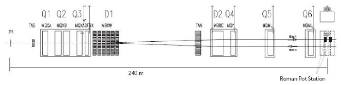
Figure 1: The LHC magnet structure close to the ATLAS Interaction Point.

The ALFA experiment consists of four detector stations placed symmetrically with respect to the ATLAS IP at 237.4 m and 241.5 m. In each station there are two roman pot devices, which allow to insert the position sensitive and triggering detectors vertically into the beam pipe. Two stations are needed at each side to be able to measure not only the scattered proton trajectory position, but also its direction (elevation angles).

An important point is to understand the dependence of the scattered proton trajectory position in the detector on its energy and momentum. It is illustrated in Figs 2a and 2b for early and nominal high $\beta^{*}$ optics, respectively. For both optics settings the impact of the $p_{y}^{\mathrm{IP}}$-momentum component at the IP on the proton position in the detector station is much greater than that due to $p_{x}^{\mathrm{IP}}$. The higher is the proton energy loss, $\Delta E$, the higher is its deflection towards the machine centre. However, due to the differences in the LHC optics for both tunes this deflection is larger in the case of the nominal high $\beta^{*}$.

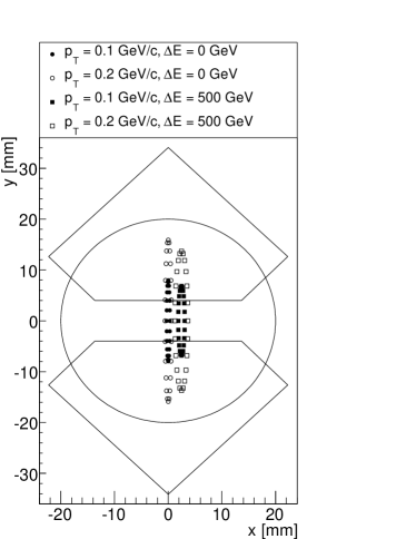
2a early high $\beta^{*}$

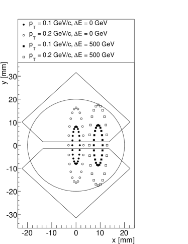
2b nominal high $\beta^{*}$

Figure 2: The positions of protons with different energy loss ($\Delta E$) and transverse momentum ($p_{T}$) at the first ALFA station for the two different LHC optics settings. The solid lines mark the beam pipe aperture and the ALFA detector active area.

Naturally, not all scattered protons can be measured in the ALFA detectors. Such proton can be too close to the beam to be detected or it can hit the LHC elements (a collimator, the beam pipe) in front of the ALFA station. The geometric acceptance, shown in Fig. 3 for both optics settings, is defined as a ratio of the number of protons of a given energy loss ($\Delta E$) and transverse momentum ($p_{T}$) that crossed the active detector area to the total number of the scattered protons having $E$ and $p_{T}$. In the calculations the following factors were taken into account: the beam properties at the IP, the beam chamber and the detector geometries, the distance between the detector edge and the beam centre. This distance was set 4 and 1.5 mm – the values expected for the early and nominal high $\beta^{*}$ runs. Values of other parameters are listed in Table 1.

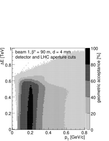
3a early high $\beta^{*}$

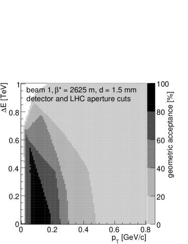
3b nominal high $\beta^{*}$

Figure 3: The geometrical acceptance of the ALFA detector as a function of the proton energy loss ($\Delta E$) and its transverse momentum ($p_{T}$) for two LHC settings. The distance between the beam centre and the detector edge was set to 4 mm for early high $\beta^{*}$ and for 1.5 mm for nominal high $\beta^{*}$.

Table 1: The LHC beam parameters at the ATLAS IP for early and nominal high $\beta^{*}$ runs.

Parameter	Unit	Early High $\beta^{*}$	Nominal High $\beta^{*}$
$\sigma_{x_{\mathrm{IP}}}$, $\sigma_{y_{\mathrm{IP}}}$	mm	0.3	0.612
$\sigma_{x_{\mathrm{IP}}^{\prime}}$, $\sigma_{y_{\mathrm{IP}}^{\prime}}$	$\mu$rad	3.33	0.233
$\sigma_{p_{T}}$	MeV/c	11.7	1.6

As can be observed, the region of acceptance above 80% is limited by $\Delta E<0.6$ TeV and $160$ MeV/c $<p_{T}<$ 200 MeV/c for early high $\beta^{*}$. If the requirement on the acceptance value is lowered to 60% then the range of the accepted transverse momentum values gets slightly larger. In the case of the nominal high $\beta^{*}$ the high acceptance region is a triangle-like and spans a bit larger range of the proton transverse momentum. Moreover, it is worth mentioning that high $\beta^{*}$ runs will have very low both instantaneous and integrated luminosities. This implies that only a few events containing particles particles with high energy loss are expected to be observed. Therefore, the most important factor is the accepted $p_{T}$ range for small $\Delta E$.

The minimum transverse momentum of protons that can be registered depends on the distance between the detector edge and the beam centre. This is demonstrated in Fig. 4 where the scattered proton transverse momentum spectra are shown for different distances and both machine settings. Clearly, the smaller the distance between the beam and the detector, the smaller is the limiting value of the accepted proton’s $p_{T}$. This is particularly important for the elastic scattering measurement where the possibility of reaching as small $p_{T}$ values as possible is crucial.

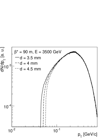
4a early high $\beta^{*}$

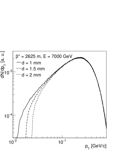
4b nominal high $\beta^{*}$

Figure 4: The influence of the distance between the detector edge and the beam centre on the accepted proton transverse momentum.

3 Transport Parametrisation

Anticipated positions of protons at the detector for a given momentum can be obtained from the transport simulation. One can also prepare a look-up table and interpolate the positions. The disadvantage of the above methods is either a long calculation time as in the first case or very extensive use of the computer storage (as size of the looking table grows with the required precision) in the second. The alternative is to use the transport parameterisation, which is very fast and requires only very little memory space. Moreover, the parameterisation provides an analytical representation of the proton position and momentum. This idea was first proposed in [7].

The LHC magnetic structure in the vicinity of the ATLAS detector is described only by the drift spaces, the dipole and the quadrupole magnets (cf. Fig. 1 or [8]). Therefore, a linear transport approximation can be applied to describe the scattered proton transport.

For a transverse variable ${\zeta}\in\{x,y,x^{\prime},y^{\prime}\}$ the transport can be effectively described by the following equations:

$$\zeta = A_{\zeta}+B_{\zeta}\cdot x_{\mathrm{IP}}+C_{\zeta}\cdot y_{\mathrm{IP}}+D_{\zeta}\cdot z_{\mathrm{IP}}+E_{\zeta}\cdot x_{\mathrm{IP}}^{\prime}$$

$$+F_{\zeta}\cdot y_{\mathrm{IP}}^{\prime}+G_{\zeta}\cdot z_{\mathrm{IP}}\cdot x_{\mathrm{IP}}^{\prime}+H_{\zeta}\cdot z_{\mathrm{IP}}\cdot y_{\mathrm{IP}}^{\prime},$$

where $A_{\zeta},\ldots,H_{\zeta}$ are the polynomials in the reduced energy loss ($\xi=\Delta E/E_{beam}$) of rank $k_{A_{\zeta}},\ \ldots,\ k_{H_{\zeta}}$:

$$A_{\zeta}=\sum_{n=0}^{k_{A_{\zeta}}}a_{{\zeta},n}\cdot\xi^{n},\ \ \ldots,\ \ H_{\zeta}=\sum_{n=0}^{k_{H_{\zeta}}}h_{{\zeta},n}\cdot\xi^{n}.$$

The absence of magnets with multipole field expansion moments higher than the quadrupole one implies that the horizontal trajectory position (direction) does not depend on the vertical momentum component nor the vertical vertex coordinate, and vice versa. The best description of the scattered proton transport for the ALFA detectors is given by:

$$\left.\begin{array}[]{ccl}x&=&\sum\limits_{n=0}^{k_{A_{x}}}a_{x,n}\cdot\xi^{n}+\sum\limits_{n=0}^{k_{B_{x}}}b_{x,n}\cdot\xi^{n}\cdot x_{\mathrm{IP}}+\sum\limits_{n=0}^{k_{E_{x}}}e_{x,n}\cdot\xi^{n}\cdot x_{\mathrm{IP}}^{\prime},\\ y&=&\sum\limits_{n=0}^{k_{C_{y}}}c_{y,n}\cdot\xi^{n}\cdot y_{\mathrm{IP}}+\sum\limits_{n=0}^{k_{F_{y}}}f_{y,n}\cdot\xi^{n}\cdot y_{\mathrm{IP}}^{\prime},\\ x^{\prime}&=&\sum\limits_{n=0}^{k_{A_{x^{\prime}}}}a_{x^{\prime},n}\cdot\xi^{n}+\sum\limits_{n=0}^{k_{B_{x^{\prime}}}}b_{x^{\prime},n}\cdot\xi^{n}\cdot x_{\mathrm{IP}}+\sum\limits_{n=0}^{k_{E_{x^{\prime}}}}e_{x^{\prime},n}\cdot\xi^{n}\cdot x_{\mathrm{IP}}^{\prime},\\ y^{\prime}&=&\sum\limits_{n=0}^{k_{C_{y^{\prime}}}}c_{y^{\prime},n}\cdot\xi^{n}\cdot y_{\mathrm{IP}}+\sum\limits_{n=0}^{k_{F_{y^{\prime}}}}f_{y^{\prime},n}\cdot\xi^{n}\cdot y_{\mathrm{IP}}^{\prime},\end{array}\right\}$$ (2)

The exact values of the coefficients were found by fitting Eq. (3) to the MAD-X PTC results. This parameterisation was validated with an independent single diffractive event sample generated with Pythia 6.4 Monte Carlo [9]. In the simulation the interaction vertex position was smeared appropriately for the discussed LHC tunes (see Tab. 1). The parametrisation uncertainty was evaluated comparing the results obtained with Eq. (2) to those of the MAD-X PTC. Results of this comparison are presented in Table 2. The differences between the MAD-X PTC and the parametrisation results are much smaller than the detector resolution (30 $\mu$m). This confirms that the parametrisation provides a good description of the scattered proton trajectory positions and elevation angles at the detectors positions.

Table 2: The parameterisation method uncertainty measured as the RMS of the difference between values given by MAD-X PTC and parameterisation equations for the early and nominal high $\beta^{*}$.

Variable	Unit	Early High $\beta^{*}$	Nominal High $\beta^{*}$
$\Delta x$	nm	45.1	37.9
$\Delta y$	nm	50.4	22.9
$\Delta x^{\prime}$	nrad	35.7	4.7
$\Delta y^{\prime}$	nrad	9.1	10.3

4 Unfolding Procedure

The procedure of inferring the scattered proton momentum on the basis of the detector measurements is called unfolding. This can be done in various ways, here is is performed by means of the minimisation of the following $\chi^{2}$ function:

$$\chi^{2}(\mathbf{p})=\frac{\left(x_{1}^{D}-x_{1}(\mathbf{p})\right)^{2}}{\sigma^{2}_{x}}+\frac{\left(y_{1}^{D}-y_{1}(\mathbf{p})\right)^{2}}{\sigma^{2}_{y}}+\frac{\left(x_{2}^{D}-x_{2}(\mathbf{p})\right)^{2}}{\sigma^{2}_{x}}+\frac{\left(y_{2}^{D}-y_{2}(\mathbf{p})\right)^{2}}{\sigma^{2}_{y}},$$

where $(x_{1}^{D},y_{1}^{D})$ denote the coordinates of the scattered proton trajectory position measured by the first station and $(x_{1}(\mathbf{p}),y_{1}(\mathbf{p}))$ – the coordinates calculated using the transport parametrisation for a proton with momentum $\mathbf{p}$. The variables $x_{2}^{D}$, $y_{2}^{D}$, $x_{2}(\mathbf{p})$ and $y_{2}(\mathbf{p})$ refer to the positions at the second station. The parametrisation does not describe correctly neither the losses of particles due to the beam pipe nor the collimators apertures, but this drawback is of a minor importance for solving the unfolding problem.

Results of the unfolding procedure are presented in Fig. 5. The correlations between the reconstructed and the generated value of the reduced energy loss and the transverse momentum components of the scattered proton are shown for the early high $\beta^{*}$ runs. For comparison the horizontal transverse momentum unfolding results are added. This figure presents also the influence of such experimental factors as the vertex smearing and the detector spatial resolution ($\sigma_{x}=\sigma_{y}=30\ \mu m$ is assumed). The leftmost plots in Fig. 5 confirm the quality of the parametrisation and the correctness of the unfolding procedure. If particular experimental effects are taken into account the unfolding accuracy worsens. Due to the chosen optics mode, the momentum reconstruction works better for the $y$ coordinate. The results show that in the early high $\beta^{*}$ case the vertex smearing has a major impact on the horizontal momentum reconstruction error whereas in the nominal high $\beta^{*}$ the leading effect is governed by the detector resolution. The difference in the horizontal momentum resolutions are due to the $x$-vertex spread. This is shown in Fig. 6, where a correlation between the $p_{x}$ unfolding error and the horizontal vertex coordinate is plotted. It clearly shows that the $x$-vertex spread has a much greater effect for the nominal high $\beta^{*}$ reconstruction accuracy.

Figure 5: Correlations between the true and unfolded values of reduced energy loss and transverse momentum components. The left column shows the ideal case where the measurement is perfect, whereas the influence of experimental effects, the vertex smearing and the detector resolution, are presented in the middle and right column, respectively.

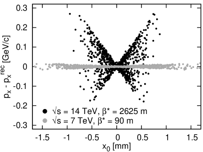
Figure 6: Left: the correlation between the horizontal momentum reconstruction error and the horizontal vertex coordinate. Right: the reduced energy loss reconstruction resolution.

It is interesting to study what precision can be obtained for measurements of the diffractively scattered protons. This would yield information on possible measurements of diffraction that can be performed with the ALFA detectors. The single diffractive dissociation events were generated with Pythia. The final state forward protons were transported to the ALFA stations and the actual positions of the trajectories were smeared according to the detector spatial resolution.

Then, the unfolding procedure was performed and its errors were estimated by fitting the distribution of the difference between the generated value and the one obtained from the unfolding with the Gaussian distribution. These fits were performed for different bins of $\xi$ (Fig. 6 right), $p_{x}$ and $p_{y}$ (Fig. 7). For comparison the momentum resolutions were calculated for the elastically scattered protons. In this case, the unfolding procedure was slightly different, because the $\chi^{2}$ minimisation was performed only in $p_{x}$ and $p_{y}$ variables as the proton energy is fixed for such events.

One immediately notices that the early high $\beta^{*}$ offers better opportunities for obtaining diffractively scattered proton kinematics. In that case the energy loss reconstruction error is about 40 GeV which compares to 160 GeV for the nominal high $\beta^{*}$. One should notice large differences between the resolutions in the horizontal and the vertical directions. This is a direct consequence of the parallel-to-point focusing optics feature dedicated to a precise measurement of small scattering angles in the vertical direction.

In the case of elastic scattering the situation is opposite: the horizontal momentum reconstruction for the nominal high $\beta^{*}$ optics has much better resolution than that for the early high $\beta^{*}$ one. The vertical momentum is reconstructed very accurately and its reconstruction resolution is about 0.3 MeV/c for both cases. This is because the nominal high $\beta^{*}$ optics is specially designed for very precise elastic scattering measurements. However, one has to remember that in the case of all high $\beta^{*}$ runs, the beam angular spread can be a serious limiting factor (cf. Tab. 1). For example, for the early high $\beta^{*}$ tune the beam transverse momentum spread is about 20 times bigger than the $p_{y}$ reconstruction resolution.

Figure 7: The horizontal (left) and vertical (right) momentum resolution for elastically and diffractively scattered protons for early and nominal high $\beta^{*}$ optics.

5 Summary

The transport of the elastically and diffractively scattered protons through the LHC magnetic lattice for the high $\beta^{*}$ optics settings was described. The geometrical acceptance for the two most probable ALFA run settings: the early high $\beta^{*}$ ($E_{\mathrm{beam}}=$ 3.5 TeV, $\beta^{*}=$ 90 m, $\epsilon^{*}=2.5\ \mu$m$\cdot$rad) and the nominal high $\beta^{*}$ ($E_{\mathrm{beam}}=$ 7 TeV, $\beta^{*}=$ 2625 m, $\epsilon^{*}=$ 1 $\mu$m$\cdot$rad) was presented. Studies of the transverse momentum acceptance as a function of the detector edge distance from the beam centre reveals that the discussed $\beta^{*}$ settings are the most desirable for the luminosity determination because the region of much lower $p_{T}$ values can be accessed.

The transport parameterisation was introduced as the fastest simulation method of the particle transport through the LHC magnetic lattice, which delivers an analytical representation of the scattered proton position at the detector stations. The accuracy of this method was shown to be much better than the assumed spatial resolution of the detector.

Finally, the unfolding method was presented as a procedure to extract the scattered proton energy and momentum at the Interaction Point from its trajectory measurement at the forward detectors. The example of the ALFA case shows that the proton energy can be reconstructed with precision of about 40 GeV in the case of early high $\beta^{*}$ and about 160 GeV for the second discussed setting. The scattered proton momentum reconstruction precision is dominated by its horizontal component resolution and is about $0.15$ GeV/c for both optics. In the elastic scattering case the momentum resolution is still dominated by its horizontal component reconstruction resolution, but the nominal high $\beta^{*}$ setting allows for twenty times better precision than the early high $\beta^{*}$ one.

References

- [1] ATLAS Luminosity and Forward Physics Community: ATLAS TDR 018, CERN/LHCC/2008-004.
- [2] R. Staszewski, P. Lebiedowicz, M. Trzebiński, J. Chwastowski, A. Szczurek, Exclusive Production at the LHC with Forward Proton Tagging, accepted by APP B.
- [3] A.Faus-Golfe and A.Verdier, High-beta and very high-beta optics studies for LHC, LHC Project Note 357, 2004.
- [4] H. Burkhardt and S. White, High- Optics for the LHC, CERN-LHC-Project-Note-431, 2010.
-
[5]
H. Grote and F. Schmidt, Mad-X Program,
http://mad.web.cern.ch/mad. - [6] E. Forest, F. Schmidt, E. McIntosh Introduction to the Polymorphic Tracking Code, CERN.SL.2002.044 (AP) KEK-Report 2002-3.
- [7] R. Staszewski and J. Chwastowski Transport Simulation and Diffractive Event Reconstruction at the LHC, Nucl. Instrum. Meth. A609 (2009) 136.
-
[8]
http://proj-lhc-optics-web.web.cern.ch/proj-lhc-optics-web/. - [9] T. Sjöstrand, S. Mrenna and P. Skands PYTHIA 6.4 Physics and Manual., JHEP 05 (2006) 026.