Benchmarking ordering techniques for nonserial dynamic programming

Abstract

Five ordering algorithms for the nonserial dynamic programming algorithm for solving sparse discrete optimization problems are compared in this paper. The benchmarking reveals that the ordering of the variables has a significant impact on the run-time of these algorithms. In addition, it is shown that different orderings are most effective for different classes of problems. Finally, it is shown that, amongst the algorithms considered here, heuristics based on maximum cardinality search and minimum fill-in perform best for solving the discrete optimization problems considered in this paper.

1 Introduction

The use of discrete optimization (DO) models and algorithms makes it possible to solve many real-life problems in scheduling theory, optimization on networks, routing in communication networks, facility location in enterprize resource planing, and logistics. Applications of DO in the artificial intelligence field include theorem proving, SAT in propositional logic, robotics problems, inference calculation in Bayesian networks, scheduling, and others.
Many real-life discrete optimization problems (DOPs) contain a huge number of variables and/or constraints that make the models intractable for currently available DO solvers. Usually, such problems have a special structure, and the matrices of constraints for large-scale problems are sparse. The nonzero elements of the matrices often involve a limited number of blocks. The block form of many DO problems is usually caused by the weak connectedness of subsystems of real-world systems.
One of the promising ways to exploit sparsity for solving sparse DOPs is nonserial dynamic programming (NSDP) BerBri , Soa07 . NSDP eliminates variables of DOP using an elimination order which makes significant impact on running time. As finding an optimal ordering is NP-complete Yanna81 , heuristics are utilized in practice for finding elimination orderings. The literature has reported extensive computational results for the use of different ordering heuristics in the solution of systems of equations Amestoy96 , George73 . However, no such experiments have been reported for NSDP to date.
Given the increased recent interest in DOPs, the subject of experimental research of NSDP algorithms that utilize heuristic variable orderings is timely. In this paper, we present comparative computational results from the benchmarking of five ordering techniques, namely: minimum degree ordering, nested dissection ordering, maximum cardinality search, minimum fill-in, and lexicographic breadth-first search.

2 Nonserial Dynamic Programming Algorithm

Consider a DOP with constraints:

$$F(x_{1},x_{2},\ldots,x_{n})=\sum_{k\in K}f_{k}(Y^{k})\rightarrow\max$$ (1)

subject to the constraints

$$g_{i}(X_{S_{i}})~{}R_{i}~{}0,~{}~{}i\in M=\{1,2,\ldots,m\},$$ (2)

$$x_{j}\in D_{j},~{}~{}j\in N=\{1,\ldots,n\},$$ (3)

where
$X=\left\{x_{1},\dots,x_{n}\right\}$ is a set of discrete variables, $Y^{k}\subseteq\{x_{1},x_{2},\ldots,x_{n}\},k\in K=\left\{1,2,\ldots,t\right\},$ $t$ – number of components of objective function, $S_{i}\subseteq\{1,2,\ldots,n\},~{}R_{i}\in\{\leq,=,\geq\},i\in M$; $D_{j}$ is a finite set of admissible values of variable $x_{j},~{}~{}j\in N$. The functions $f_{k}(X^{k}),~{}~{}k\in K$ are called components of the objective function and can be defined in tabular form. We use here a notation: if $S=\{j_{1},\ldots,j_{q}\}$ then $X_{S}=\{x_{j_{1}},\ldots,x_{j_{q}}\}$.

2.1 The structure of sparse discrete optimization problems

Let us take a detailed look at an NSDP implementation for solving DO problems for the case when the structural graph is an interaction graph of variables.

Definition 1

BerBri . Variables $x\in X$ and $y\in X$ interact in DOP with constraints (we denote $x\sim y$) if they appear both either in the same component of objective function, or in the same constraint (in other words, if variables are both either in a set $X^{k}$, or in a set $X_{S_{i}}$).

Definition 2

BerBri . Interaction graph of the DOP is called an undirected graph $G=(X,E)$, such that

1. Vertices $X$ of $G$ correspond to variables of the DOP;

2. Two vertices of $G$ are adjacent if corresponding variables interact.

Further, we will use the notion of vertices that correspond one-to-one to variables.

Definition 3

Set of variables interacting with a variable $x\in X$, is denoted as $Nb(x)$ and called a neighborhood of the variable $x$. For corresponding vertices of $G$ a neighborhood of a vertex $x$ is a set of vertices of interaction graph that are linked by edges with $x$. Denote the latter neighborhood as $Nb_{G}(x)$.

In hypergraph representation of DO problems structure, the set of vertices $H$ of hypergraph, equals to the set of variables $X$ from the DO problems, and hypergraph’s hyperedges forms subsets of related variables that are included in constraints, which means the hyperedge defines constraint scope.

2.2 NSDP (Variable elimination) algorithms

Consider a sparse discrete optimization problem (1) – (3) whose structure is described by an undirected interaction graph $G=(X,E)$. Solve this problem with a NSDP.
Given ordering of variable indices $\alpha$ the NSDP proceeds in the following way: it subsequently eliminates $x_{\alpha_{1}},\dots,x_{\alpha_{n}}$ in the current graph and computes an associated local information $h_{i}(Nb(x_{\alpha_{i}}))$ about vertices from $Nb(x_{\alpha_{i}})$ ($i=1,\dots,n$). This can be described by the combinatorial elimination process:

$$G^{0}=G,G^{1},\ldots,G^{j-1},G^{j},\ldots,G^{n},$$

where $G^{j}$ is the $x_{\alpha_{j}}$-elimination graph of $G^{j-1}$ and $G^{n}=\emptyset$
The process on interaction graph transformation corresponding to the NSDP scheme is known as elimination game which was first introduced by Parter Part as a graph analogy of Gaussian elimination. The input of the elimination game is a graph $G$ and an ordering $\alpha$ of $G$.
Consider the DOP described above and suppose without loss of generality that variables are eliminated in the order $x_{1},\dots,x_{n}$ . Using the variable elimination scheme eliminate a first variable $x_{1}$. This $x_{1}$ is in a set of constraints with the indices of $U_{1}=\{i~{}|~{}x_{1}\in X_{S_{i}}\}$. Together with $x_{1}$, in constraints $U_{1}$ are variables from $Nb(x_{1})$. To the variable $x_{1}$ corresponds the following subproblem $P_{1}$:

$$h_{1}(Nb(x_{1}))=\max_{x_{1}}\Bigl{\{}\sum_{k\in K_{1}}f_{k}(Y^{k})~{}|~{}g_{i}(X_{S_{i}})~{}R_{i}~{}0,~{}~{}i\in U_{1},~{}x_{j}\in D_{j},~{}x_{j}\in Nb[x_{1}]\Bigr{\}}.$$

Then the initial DOP can be transformed in the following way:

$$\max_{x_{1},\ldots,x_{n}}\Bigl{\{}\sum_{k\in K}f_{k}(Y^{k})~{}|~{}g_{i}(X_{S_{i}})~{}R_{i}~{}0,~{}~{}i\in M,~{}x_{j}\in D_{j},~{}j\in N\Bigr{\}}=$$

$$\max_{x_{2},\ldots,x_{n}}\Bigl{\{}\sum_{k\in K-K_{1}}f_{k}(Y^{k})+h_{1}(Nb(x_{1})~{}|~{}g_{i}(X_{S_{i}})~{}R_{i}~{}0,~{}~{}i\in M-U_{1},~{}x_{j}\in D_{j},~{}j\in N-\{1\}\Bigr{\}}$$

The last problem has $n-1$ variables; from the initial DOP were excluded constraints with the indices from $U_{1}$ and objective function term $\sum_{k\in K_{1}}f_{k}(Y^{k})$; there appeared a new objective function term $h_{1}(Nb(x_{1}))$. Due to this fact the interaction graph associated with the new problem is changed: a vertex $x_{1}$ is eliminated and its neighbors have become connected.
Denote the new interaction graph $G^{1}$ and find all neighborhoods of variables in $G^{1}$. NSDP eliminated the remaining variables one by one in an analogous manner.

3 Elimination Ordering Techniques

An efficiency of the NSDP algorithm crucially depends on the interaction graph structure of a DOP. If the interaction graph is rather sparse or, in other words, has a relatively small induced width, then the complexity of the algorithm is reasonable. At the same time an interaction graph leads us to another critical factor such as an elimination order which should be obtained from the interaction graph.
From the other side the NSDP algorithm heavily depends on the elimination ordering. A good elimination ordering yields small cliques during variable elimination. There are several successful schemes for finding a good ordering which we will used in this paper: minimum degree ordering algorithm (MD), nested dissection ordering algorithm (ND), maximum cardinality search algorithm (MCS), minimum fill-in heuristic (MIN-FILL) and lexicographic breath-first search algorithm (LEX-BFS).

3.1 Minimum degree ordering algorithm

The minimum degree (MD) ordering algorithm Amestoy96 is one of the most widely used in linear algebra heuristic, since it produces factors with relatively low fill-in on a wide range of matrices.
In the minimum degree heuristic, a vertex $v$ of minimum degree is chosen. The graph $G^{\prime}$, obtained by making the neighborhood of $v$ a clique and then removing $v$ and its incident edges, is built. Recursively, a chordal supergraph $H^{\prime}$ of $G^{\prime}$ is made with the heuristic. Then a chordal supergraph $H$ of $G$ is obtained, by adding $v$ and its incident edges from $G$ to $H^{\prime}$. To create an elimination order with help of minimum degree ordering algorithm the $minimum\_degree\_ordering()$ function from BOOST library BOOST has been used.

3.2 Nested dissection algorithm

To create an elimination order, we recursively partition the elimination graph using nested dissection. More specifically, we use $METIS\_EdgeND()$ function from METIS library Karypis to find a nested dissection ordering.

3.3 Maximum cardinality search algorithm

The Maximum Cardinality Search (MCS) algorithm Tarjan84 visits the vertices of a graph in an order such that at any point, a vertex is visited that has the largest number of visited neighbors. An MCS-ordering of a graph is an ordering of the vertices that can be generated by the Maximum Cardinality Search algorithm. The visited degree of a vertex $v$ in an MCS-ordering is the number of neighbors of $v$ that are before $v$ in the ordering.
To create an elimination ordering the $chompack.maxchardsearch()$ function from the Chordal Matrix Package (CHOMPACK) CHOMPACK has been used.

3.4 Minimum Fill-in algorithm

The minimum fill-in heuristic Jegou works similarly with minimum degree heuristic, but now the vertex $v$ is selected such that the number of edges that is added to make a neighborhood of $v$ a clique is as small as possible.

3.5 Lexicographic breadth-first search algorithm

Lexicographic breadth-first search algorithm (LEX-BFS) Rose76 numbers the vertices from $n$ to 1 in the order that they are selected. This numbering fixes the positions of an elimination scheme. For each vertex $v$, the label of $v$ will consist of a set of numbers listed in decreasing order. The vertices can then be lexicographically ordered according to their labels.

4 Benchmarking

4.1 NSDP algorithm implementation

The NSDP algorithm was implemented by the first author in Python. The ND and MD algorithms were implemented in C and C++, respectively. To work with graph objects was taken class networkx.Graph from the networkx library NetworkX .

4.2 Test problems

For benchmarking the DO test problems were generated by using hypergraphs from the CSP hypergraph library Musliu . This collection contains various classes of constraint hypergraphs from industry (DaimlerChrysler, NASA, ISCAS) as well as synthetically generated ones (e.g. Grid or Cliques).
The test problems were generated in the following way. The constraints structure of a linear DO problem with binary variables was described by hypergraph from the library Musliu . To build constraint $i$ the next hyperedge of hypergraph was taken, which includes a set of variables $X_{S_{i}}$ for a new building constraint. In the next step, the coefficients for appropriate variables of $A_{S_{i}}$ were generated using a random number generator. Then the left part of $i$-th constraint had view $A_{S_{i}}X_{S_{i}}$, while the right part was $\sigma\sum A_{S_{i}}$, where $\sigma$ is random number from interval (0, 1). Objective function is linear and includes all variables – vertices of hypergraph, where coefficients $c_{j}$ of objective function $\sum_{j=1}^{n}c_{j}x_{j}\rightarrow\max$ where created with help of random number generator.
After the test problems were generated, the ordering algorithms MD, ND, MCS, MIN-FILL and LEX-BFS were applied for obtaining an elimination ordering. Then the problems were solved with the NSDP algorithm by utilizing to the specified elimination ordering.

4.3 Benchmarking ordering analysis

The following five groups of 33 test problems have been taken: ’dubois’, ’bridge’, ’adder’, ’pret’ and ’NewSystem’. All experimental results were obtained on a machine with Intel Core 2 Duo processor 2.66 GHz, 2 GB main memory and operating system Linux, version 2.6.35-24-generic. The results can be found in table 1, in which $n$ denotes the number of variables, $m$ the number of constraints and the minimal time of problem solving for appropriate heuristics was underlined. We can see that for ND algorithm the minimal run-time of the NSDP algorithm was achieved 0 times (0 %), for MD 2 times (6,0 %), LEX-BFS 3 times (9,1 %), MCS 9 times (27,3 %) and MIN-FILL 19 times (57,6 %).

Table 1: Run-time (in seconds) of solving DO problems with help of NSDP algorithm using different orderings.

Test	$n$	$m$	MD	ND	MCS	MIN-FILL	LEX-BFS
dubois20	60	40	1,31	1,43	1,17	1,19	1,20
dubois21	63	42	1,52	1,67	1,35	1,31	1,35
dubois22	66	44	1,37	1,70	1,51	1,51	1,49
dubois23	69	46	1,90	2,02	1,70	1,68	1,74
dubois24	72	48	2,18	2,17	1,89	1,80	1,95
dubois25	75	50	2,72	2,50	2,11	2,14	2,15
dubois26	78	52	2,62	2,82	2,32	2,43	2,39
dubois27	81	54	2,58	3,09	2,60	2,71	2,66
dubois28	84	56	3,55	3,43	2,90	2,84	2,98
dubois29	87	58	3,91	3,84	3,22	3,21	3,28
dubois30	90	60	4,46	4,14	3,50	3,52	3,48
dubois50	150	100	17,52	16,31	14,34	14,00	14,53
dubois100	300	200	126,32	111,64	106,34	103,23	106,29
adder_15	106	75	6,20	7,04	5,25	5,64	5,38
adder_25	176	125	27,33	32,13	21,47	24,27	23,10
adder_50	351	250	326,54	388,74	268,39	276,47	254,25
adder_75	526	375	4876,74	5180,46	3381,28	3460,32	3435,76
bridge_15	137	135	15,21	15,41	13,90	12,45	12,86
bridge_25	227	225	63,14	74,18	62,30	55,98	58,62
bridge_50	452	450	900,20	983,40	922,68	886,91	1003,89
bridge_75	677	675	4832,55	5049,61	4507,38	3886,34	5040,91
pret60_25	60	53	1,89	1,51	1,68	1,32	1,59
pret60_40	60	53	1,50	1,48	1,69	1,26	1,52
pret60_60	60	53	1,58	1,51	1,83	1,27	1,64
pret60_75	60	53	1,44	1,60	1,79	1,31	1,54
pret150_25	150	133	21,29	33,06	20,51	16,25	23,04
pret150_40	150	133	22,63	32,83	21,47	16,44	24,76
pret150_60	150	133	22,09	31,13	23,72	16,35	23,99
pret150_75	150	133	21,20	33,23	20,19	18,57	23,59
NewSystem1	142	85	19,21	16,24	14,05	17,33	14,08
NewSystem2	345	200	603,83	520,82	376,33	489,80	425,35
NewSystem3	474	284	1294,86	1352,75	1159,75	1247,81	1072,58
NewSystem4	718	422	7769,10	8322,58	6427,85	7095,17	6845,20

Let us take a look at the benchmarking results in more detail. Fig. 1 describes results of the experiment for the groups of test problems ’dubois’, ’bridge’, and ’adder’. These results show to us that MCS, MIN-FILL and LEX-BFS heuristics behave quite similar and give the best result for a given group of problems. At the same time MD and ND show the worst time result. Also for the group ’bridge’ we can see the gradual decreasing of the time result for the LEX-BFS heuristics and the obvious domination of MIN-FILL.

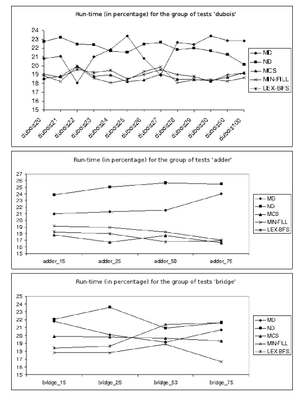
Figure 1: Run-time (in seconds) for groups of tests ’dubois’, ’adder’, ’bridge’.

Fig. 2 describes experimental results for the groups of test problems ’pret’ and ’NewSystem’.

Figure 2: Run-time (in seconds) for groups of tests ’pret’ and ’NewSystem’.

Here we can see the importance of the right choice of heuristics for a certain group of problems. In the case of ’pret’, we see obvious domination of MIN-FILL algorithm, while MCS and LEX-BFS fall behind. However, the group ’NewSystem’ shows completely opposite results, where MIN-FILL runs third while MCS and LEX-BFS take the first two places.
In the case of ’pret’, we see the obvious domination of the MIN-FILL algorithm, while MCS and LEX-BFS go back. But the group ’NewSystem’ shows the completely opposite result, where MIN-FILL goes on the third place while MCS and LEX-BFS take the first places.

5 Conclusion

The goal of this paper to research the role of five variable ordering algorithms and to describe the effect that they play on solving time of sparse DO problems with help of NSDP algorithm. Our computational experiments demonstrate that, for solving DO problems, variable ordering has a significant impact on the run-time for solving the problem. Furthermore, different ordering heuristics were observed to be more effective for different classes of problems. Overall, the MCS and MIN-FILL heuristics have provided the best results for solving DO problems of the problem classes that were considered in this paper. It seems promising to continue this line of research by studying methods of block elimination with suitable partitioning methods.

References

- (1) Amestoy PR, Davis TA, Duff IS, An approximate minimum degree ordering algorithm, SIAM Journal on Matrix Analysis and Applications, V. 17, N 4, 886-905 (1996)
- (2) Bertele U, Brioschi F, Nonserial Dynamic Programming, 235 p. Academic Press, New York (1972)
-
(3)
BOOST, minimum degree ordering algorithm.
http://www.boost.org/doc/libs/1_46_1/libs/graph/doc/minimum_degree_ordering.html. - (4) CHOMPACK, maximum cardinality ordering algorithm. URL: http://abel.ee.ucla.edu/chompack/
- (5) George JA, Nested dissection of a regular finite element mesh, SIAM J Numer Anal, V. 10, 345-367 (1973)
- (6) Jégou P, Ndiaye SN, Terrioux C, Computing and exploiting tree-decompositions for (Max-)CSP, Proceedings of the 11th International Conference on Principles and Practice of Constraint Programming (CP-2005), P. 777-781 (2005)
- (7) Karypis G, Kumar V, MeTiS a software package for partitioning unstructured graphs, partitioning meshes, and computing fill-reducing orderings of sparse matrices. Version 4. University of Minnesota (1998)
- (8) Musliu N, Samer M, Ganzow T, Gottlob G, A csp hypergraph library, Technical Report, DBAI-TR-2005-50, Technische Universität Wien (2005)
- (9) NetworkX is a Python package for the creation, manipulation, and study of the structure, dynamics, and functions of complex networks. http://networkx.lanl.gov/
- (10) Parter S, The use of linear graphs in Gauss elimination, SIAM Review, 3, 119-130 (1961)
- (11) Rose DJ, Tarjan R, Lueker G, Algorithmic aspects of vertex elimination on graphs, SIAM J Comput, V. 5, 266-283 (1976)
- (12) Shcherbina O, Nonserial dynamic programming and tree decomposition in discrete optimization, Proceedings of Int. Conference on Operations Research ”Operations Research 2006” (Karlsruhe, 6-8 September, 2006), Springer Verlag, Berlin (2007), 155-160
- (13) Tarjan RE, Yannakakis M, Simple linear-time algorithms to test chordality of graphs, test acyclity of hypergraphs, and selectively reduce acyclic hypergraphs, SIAM J Comput, V. 13, 566-579 (1984)
- (14) Yannakakis M, Computing the minimum fill-in is NP-complete. SIAM J Alg Disc Meth, V. 2, 77-79 (1981)