Emergence of hierarchical networks and polysynchronous behaviour in simple adaptive systems

Abstract

We describe the dynamics of a simple adaptive network. The network architecture evolves to a number of disconnected components on which the dynamics is characterized by the possibility of differently synchronized nodes within the same network (polysynchronous states). These systems may have implications for the evolutionary emergence of polysynchrony and hierarchical networks in physical or biological systems modeled by adaptive networks.

Graphs or networks are used to describe the evolution and interaction of coupled systems. Each node is assumed to have an underlying dynamics which can be affected by ‘neighbouring’ nodes. This influence is represented by a directed edge, or arrow, indicating input from one node to another in the direction of the arrow. This can be complicated by allowing the neighbours of a node to vary with time as a function of the state of the nodes, giving rise to adaptive networks Gross and Blasius (2008); Gross and Sayama (2009). These models have been applied to a broad range of problems including the connectivity of the internet, the social interactions in a community and motifs in systems biology, see Boccaletti et al. (2006); Milo et al. (2002); Gross and Blasius (2008); Gross and Sayama (2009) for further details and examples.

The dynamics of these systems can be rich, both in terms of the temporal dynamics at the nodes and the emergence of topological structure in the networks. For example, the dynamics can synchronize, so all nodes behave asymptotically in the same way Pikovsky et al. (2003). Polysynchrony describes a more subtle form of synchronization Stewart et al. (2003); Golubitsky et al. (2004); Field (2004); Aguiar et al. (2009); Agarwal and Field (2010) where groups of nodes can be synchronized and, unlike cluster synchronization, synchronized nodes need not be connected to each other.

The aim of this note is to show that complicated polysynchronous dynamics can emerge in adaptive networks using a simple homophilic principle to determine the evolution of the links of the network. This is based on the idea that nodes ‘like’ being connected to similar nodes, a common assumption in many socially motivated networks and a basic principle in neural network dynamics. In other words we consider a collection of identical individuals operating under the same homophilic rules, and show that the system evolves to a finite number of connected components, each of which can display polysynchronous states. All the examples we have looked at have a further interesting property: the final states have graphs which have a hierarchical structure, with a group of strongly connected components at the bottom, and then the remaining nodes being arranged above these (taking information from them, but not giving information) in levels reflecting the number of directed links needed to get to the node from one of the bottom nodes or ‘roots’. (Note that we say a set of nodes is strongly connected if there is a path in the graph following the directed edges or arrows between any two nodes, and connected if there is a path between any two nodes following edges, so the path can use an edge in the opposite direction to the arrow.) This suggests that polysynchrony and hierarchy are natural states that can emerge from simple undifferentiated networks over time. We will discuss further implications of this towards the end of the article.

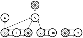
Figure 1: Example of a polysynchrony pattern ($N=10$, $\varepsilon=0.85$). In this case the node dynamics have been attracted to two different fixed points. Nodes filled with the same pattern are synchronized including the isolated pair $\{6,9\}$. Arrows have an associated weight and equation (2) tells us that, for each node, the weights of all incoming arrows sum up to $m=N-1$. Since a node always get its inputs from only one synchrony class, we have avoided labelling the weights for the sake of clarity.

Before describing our model in full detail it is worth looking at a couple of examples to illustrate the results. The first (Fig. 1) shows the final state of our system below with ten nodes. The final graph has broken into two subsystems; one containing two nodes and the other eight nodes. The eight node subsystem has two basic strongly connected sets, $\{1,2,8\}$ and $\{7,10\}$, and these influence but are not influenced by nodes 4 and 5, which in turn influences node 3. There are two polysynchrony classes: the dynamics of nodes $\{2,4,5,9,10\}$ is identical as is that of the remaining nodes. At first sight this appears remarkable as the nodes in the isolated pair $\{6,9\}$ are also part of the same polysynchrony classes. We explain this below. In this case the dynamics is trivial: two fixed points, one for each polysynchrony class, but more complicated behaviour is possible as shown in Fig. 2.

Figure 2: Example of a polysynchrony pattern ($N=10$, $\varepsilon=0.8$). The node dynamics are chaotic in this case. Nodes filled with the same pattern are synchronized.

The final state in Fig. 2 is a chain based on two interacting nodes at the root with polysynchrony classes that oscillate up the chain. The dynamics of each polysynchrony class is chaotic, but each element of the same class is fully synchronized.

To summarize from these two observations: the dynamics breaks up into a small number of disconnected sets, and within each of these sets the dynamics may be either simple (a fixed point in the first example) or more complicated (chaotic in the second example), and in fact we will show that different behaviours across polysynchrony classes in the same connected component are also possible. Contrary to full synchronization or cluster synchronization, the synchronized nodes have no direct links connecting them. Moreover the final graphs have a hierarchical structure, lending themselves to interpretation as motifs as they allow a well-defined sense of input and output nodes.

The model consists of a directed network of $N$ nodes. The dynamics of the $i$th ($i=1,\dots,N$) node are given by

$$x^{i}_{n+1}=f(x^{i}_{n})+\frac{\varepsilon}{m}\sum_{j=1}^{N}A^{ij}_{n}(f(x^{j}_{n})-f(x^{i}_{n}))$$ (1)

where we choose $f$ to be the fully-chaotic logistic map $f(x)=4x(1-x)$ and $A_{n}$ is the adjacency matrix of the network at time step $n$, so $A^{ij}_{n}=k$ if there are $k$ connections (directed edges) from $j$ to $i$, with the direction indicated by the arrow in the accompanying figures. Each node is assigned a fixed number $m$ of incoming links so

$$\sum_{j=1}^{N}A^{ij}_{n}=m,$$ (2)

and we choose $m=N-1$ throughout this paper. These links can be rewired at each iteration following an algorithm that will be described below.

At each iteration the $i$th node is influenced by the dynamics of those nodes to which it is connected by an incoming arrow. We will call these nodes the neighbours of node $i$. Due to the condition imposed by (2), a node can have at most $m$ neighbours.

We describe now the rewiring mechanism. At each iteration $n$ we compute the distance matrix $D^{ij}_{n}$

$$D^{ij}_{n}=\left\{\begin{tabular}[]{ll}$|f(x^{i}_{n})-f(x^{j}_{n})|$,&\ \ $A^{ij}_{n}\neq 0$\\ $0$,&\ \ $A^{ij}_{n}=0$\end{tabular}\right.$$ (3)

and calculate from it the mean distance of a node to all its neighbours

$$\langle D\rangle^{i}_{n}=\frac{1}{a^{i}_{n}}\sum_{j=1}^{N}D^{ij}_{n}$$ (4)

where $a^{i}_{n}$ is the unweighted number of neighbours of node $i$ at time step $n$, i.e. the sum over $j$ of ${\rm sign}(A^{ij}_{n})$.

For the rewiring we apply a homophilic principle: nodes prefer to be connected to nodes being in a similar state. We identify the bad neighbours $j\in\mathcal{B}^{i}_{n}$ of each node $i$ at iteration $n$ with the following criterion

$$j\in\mathcal{B}^{i}_{n}\quad\text{if}\quad D^{ij}_{n}>\langle D\rangle^{i}_{n},$$ (5)

so a neighbour $j$ is considered bad if its distance $D^{ij}_{n}$ to the node is larger than the average distance of the neighbourhood $\langle D\rangle^{i}_{n}$. The good neighbours of node $i$ are then given by

$$\mathcal{G}^{i}_{n}=\{1,\dots,N\}\backslash\left(\mathcal{B}^{i}_{n}\cup\{i\}\right),$$ (6)

so $i\notin\mathcal{G}^{i}_{n}$ which means that a node never becomes linked to itself. Once the good and bad neighbours have been identified node $i$ will break the links coming from $\mathcal{B}^{i}_{n}$ and randomly rewire them to nodes in $\mathcal{G}^{i}_{n}$. Let $b^{i}_{n}$ be the number of bad neighbours

$$b^{i}_{n}=\sum_{j\in\mathcal{B}^{i}_{n}}A^{ij}_{n}.$$ (7)

Now choose $b^{i}_{n}$ elements of $\mathcal{G}^{i}_{n}$ at random and suppose that $r^{ik}_{n}$ is the number of times node $k$ is chosen. The adjacency matrix at the next time step is

$$A^{ik}_{n+1}=\left\{\begin{tabular}[]{ll}$0$,&$k\in\mathcal{B}^{i}_{n}$\\ $A^{ik}_{n}+r^{ik}_{n}$,&$k\in\mathcal{G}^{i}_{n}$\end{tabular}\right..$$ (8)

In all the cases described here the initial connectivity is the symmetric all-to-all connectivity where each node in the network is connected to all the possible $m=N-1$ neighbours and $A_{0}^{ii}=0$.

The first main observation is that, at least for systems of moderate size, the rewiring dynamics always settles down to a frozen state after a finite amount of time. This is possible due to the criterion used to perform the rewiring of the links at each iteration. If at time step $n$, a node $i$ has all its incoming links coming from the same node or from a synchronized set of neighbours, all elements in the distance matrix $D^{ij}_{n}$ will have the same value ($D^{ij}_{n}=\langle D\rangle^{i}_{n}$ for all $j$ such that $A^{ij}_{n}\neq 0$) resulting in an empty set of bad nodes and hence ‘locking’ node $i$ to its neighbourhood for the next time step. However, we should notice the locking process is not purely probabilistic because the interactions between the nodes correlate their dynamics thus affecting the locking probabilities.

The second and most important observation is that, as Fig. 3 shows, the dynamics of the nodes once the network has frozen has a high probability of being polysynchronous for a wide range of coupling strengths, namely $0.75<\varepsilon<1$ and also $0.12\lesssim\varepsilon\lesssim 0.2$. There are other possible dynamics for this adaptive network model depending on the value of the coupling strength including uncorrelated dynamics (no two nodes are synchronized), full synchronization (all the nodes in the network synchronize) and cluster or partial synchronization, but in the regions of parameter space that we have identified, polysynchronous and hierarchical states appear most frequently.

As studied in Stewart et al. (2003) the network needs to satisfy some symmetry requirements in order to achieve robust polysynchrony. The structure of polysynchronous networks requires a balanced equivalence relation to be established on the nodes, so the nodes can be separated into equivalence classes of nodes with equivalent inputs. For example, in Fig. 1 none of the nodes in the same synchrony class have links connecting them to each other, but receive all their $m$ inputs from nodes in the other synchrony class. In principle, a more general input equivalence could be established in which nodes in a certain synchrony class receive inputs from various synchrony classes (including inputs from their own synchrony class) Golubitsky et al. (2005). However, using arguments similar to those for the locking mechanism we can show that this is not possible in our model due to the homophilic rewiring criterion chosen: if a node receives inputs from two different synchrony classes a certain time step $n$ then typically the distance from these sets will be different and all the links from one class will be rewired at the next time step Botella-Soler and Glendinning (2011). We have taken advantage of this property of the model to assess the polysynchronous character of the final network by comparing the final difference ($\delta^{ij}_{n}=|x^{i}_{n}-x^{j}_{n}|$) and adjacency matrices. If all the non-diagonal $0$ elements in the difference matrix (which reflect synchrony between two nodes) correspond to non-connected nodes (reflected by $0$ elements in the adjacency matrix) then our network is polysynchronous.

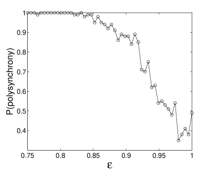
Figure 3: Probability of polysynchrony as a function of the coupling strength $\varepsilon$. $N=10$, 100 initial conditions have been evaluated for each value of $\varepsilon$. Polysynchrony has been identified as explained in the text.

A further characteristic of the networks showing polysynchrony in our model is that their structure is usually strongly hierarchical. If we define the set of nodes in strongly connected components to be the ‘roots’ of the network (for instance, nodes 2 and 8 are the root of the network in Fig. 2) then the ‘level’ of a node is the minimum (directed) path length from the root to the node, and the ‘height’ of a node is the average distance over all possible directed paths from the root to the node. These concepts are inspired by the definitions of ‘trophic level’ and ‘trophic height’ introduced for the study of food webs Quince et al. (2005), and our choice of the root ensures that the level and height are well-defined Botella-Soler and Glendinning (2011). We say that a network is strongly hierarchical if level and height coincide for all the nodes in the network. One can see this definition applies to the networks in Fig. 1 and 2. Another example of strongly hierarchical polysynchronous network is shown in Fig. 4 where the root is composed of two strongly connected pairs. This example has the additional interest that different synchrony classes inside the same cluster show different dynamical behaviour. While the root pairs $\{5,10\}$ and $\{4,6\}$ follow a period-2 cycle, the rest of the nodes in the network show period-4 dynamics. Moreover, it is interesting to note that nodes in classes {4,5} and {1,3,8,9} all receive the same input (from class {6,10}) but show different dynamics. This illustrates that having equivalent inputs is only a necessary but not sufficient condition to be in the same synchrony class Golubitsky et al. (2006).

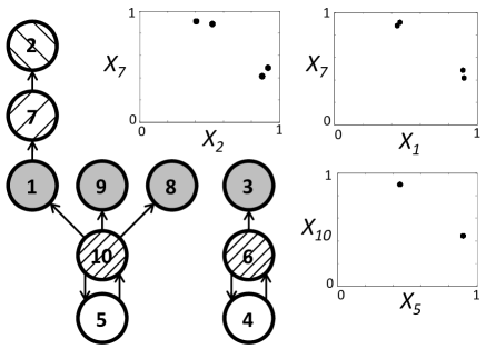
Figure 4: Example of a polysynchronous pattern ($N=10$, $\varepsilon=0.14$). In this case there are 4 different synchrony classes showing 2 different dynamical behaviours: $\{4,5\}$ and $\{6,10\}$ are synchronized in a period-2 cycle while $\{2\}$,$\{7\}$ and $\{1,3,8,9\}$ show period-4 dynamics.

Finally, note that since an element of a given polysynchrony class receives its inputs from a given other synchrony class, the equations determining the dynamics of each polysynchrony node are the same. This implies that the after identifying all nodes in the same polysynchrony class the dynamics is based on a very small number of possibilities: we conjecture that these quotient systems are based on rings (sometimes with additional spokes as in Fig. 4). This explains the synchrony across the unconnected components of Fig. 1 – the quotient dynamical systems are identical – a connected pair – and the dynamics has no phase information as it is just made up of fixed points. If the dynamics is more complicated then phase information can be different in different connected components with the same quotient system, see Botella-Soler and Glendinning (2011) for more details.

The emergence of polysynchrony in networks of undifferentiated nodes operating with a simple homophilic dynamic evolution suggests natural mechanisms for the emergence of polysynchrony in nature. Combining this with an additional slow timescale dynamics to describe the evolution of differentiated polysynchronous states over time would provide a way of locking in the polysynchronous pattern making it more stable to perturbation, or alternatively the evolutionary dynamics could select the appropriate polysynchronous patterns if only some subset of the possible patterns is advantageous to the system. We have reported results with relatively low numbers of nodes. As the number of nodes increases transient times increase significantly, and so evolutionary time scales could become comparable to the time of approach to the frozen state, and this may provide another way whereby evolution and differentiation or speciation can interact, although numerical simulation then becomes harder. The hierarchical nature of the asymptotic networks imply that they could operate as motifs, with a well defined input and output level, so in this case our model may provide a mechanism for functional differentiation. Models similar to the one proposed here are used to describe metapopulations Parthasarathy and Guemez (1998) so there may also be applications in this area.