Cellular buckling from mode interaction in I-beams under uniform bending

Abstract

Beams made from thin-walled elements, whilst very efficient in terms of the structural strength and stiffness to weight ratios, can be susceptible to highly complex instability phenomena. A nonlinear analytical formulation based on variational principles for the ubiquitous I-beam with thin flanges under uniform bending is presented. The resulting system of differential and integral equations are solved using numerical continuation techniques such that the response far into the post-buckling range can be portrayed. The interaction between global lateral-torsional buckling of the beam and local buckling of the flange plate is found to oblige the buckling deformation to localize initially at the beam midspan with subsequent cellular buckling (snaking) being predicted theoretically for the first time. Solutions from the model compare very favourably with a series of classic experiments and some newly conducted tests which also exhibit the predicted sequence of localized followed by cellular buckling.

1 Introduction

Beams are possibly the most common type of structural component, but when made from thin metallic plate elements they are well known to suffer from a variety of elastic instability phenomena. There has been a vast amount of research into the buckling of thin-walled structural components with much insight gained [1, 2, 3]. In the current work, the well-known problem of a beam made from a linear elastic material with an open and doubly-symmetric cross-section – an “I-beam” – under uniform bending about the strong axis is studied in detail. Under this type of loading, long beams are primarily susceptible to a global mode of instability namely lateral-torsional buckling (LTB), where, as the name suggests, the beam deflects sideways and twists once a threshold critical moment is reached [4]. However, when the individual plate elements of the beam cross-section, namely the flanges and the web, are relatively thin or slender, elastic local buckling of these may also occur; if this happens in combination with global instability, then the resulting behaviour is usually far more unstable than when the modes are triggered individually. Other structural components, usually those under axial compression rather than uniform bending, such as I-section struts with thin plate flanges [5], sandwich struts [6], stringer-stiffened and corrugated plates [7, 8] and built-up, compound or reticulated columns [9] are all known to suffer from so-called interactive buckling phenomena where the global and local modes of instability combine nonlinearly.

Experimental evidence suggests that the destabilization from the mode interaction of LTB and flange local buckling is severe [10, 11], the response being highly sensitive to geometric imperfections particularly when the critical loads coincide [12, 13]. Nevertheless, apart from the aforementioned work where some successful numerical modelling (both finite strip and finite element) and qualitative modelling using rigid links and spring elements were presented, the formulation of a mathematical model accounting for the interactive behaviour has not been forthcoming. The current work presents the development of a variational model that accounts for the mode interaction between global LTB and local buckling of a flange such that the perfect elastic post-buckling response of the beam can be evaluated. A system of nonlinear ordinary differential equations subject to integral constraints is derived, which are solved using the numerical continuation package Auto [14]. It is indeed found that the system is highly unstable when interactive buckling is triggered; snap-backs in the response showing sequential destabilization and restabilization and a progressive spreading of the initial localized buckling mode are also revealed. This latter type of response has become known in the literature as cellular buckling [15] or snaking [16] and it is shown to appear naturally in the numerical results of the current model. As far as the authors are aware, this is the first time this phenomenon has been found in beams undergoing LTB and local buckling simultaneously. Similar behaviour has been discovered in various other mechanical systems such as in the post-buckling of cylindrical shells [17, 18] and the sequential folding of geological layers [19, 20].

Experimental results generated for the current study and from the literature are compared with the results from the presented model; highly encouraging quantitative results emerge both in terms of the mechanical destabilization exhibited and the nature of the post-buckling deformation with tangible evidence of cellular buckling being found. This demonstrates that the fundamental physics of this system is captured by the analytical approach. A brief discussion is presented on whether other structural components made from thin-walled elements may also exhibit cellular buckling when local and global modes of instability interact. Conclusions are then drawn.

2 Variational formulation

2.1 Classical critical moment derivation via energy

Consider a uniform simply-supported (pinned) doubly-symmetric I-beam of length $L$ made from an isotropic and homogeneous linear elastic material with Young’s modulus $E$ and Poisson’s ratio $\nu$. The overall beam height and flange widths are $h$ and $b$ respectively with the web and flange thicknesses being $t_{w}$ and $t_{f}$ respectively. The beam is under bending about the strong axis with a uniform moment $M$, as shown in Figure 1(a).

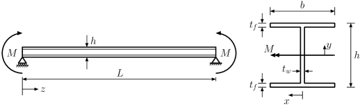
(a) Beam geometry: elevation (left) and cross-section (right)

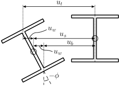
(b) LTB displacements

Figure 1: (a) An I-section beam under uniform strong axis moment $M$. (b) Lateral displacements and torsional rotations due to LTB. A right-hand Cartesian coordinate system is employed.

The second moments of area about the strong and weak axes are defined as $I_{x}$ and $I_{y}$ respectively. When LTB occurs, as noted in the literature [4], the strong axis bending moment and corresponding displacements only couple with the lateral displacements and torsional rotations at higher orders. For this reason and for the sake of simplicity, the displacements arising from strong axis bending are presently neglected, which is a common assumption; in future work, however, these coupling effects may be incorporated. Therefore, only two separate lateral displacements are defined for determining the respective positions of the local centroids of the web and the flanges: $u_{s}$ and $u_{w}$. The lateral displacements of the top ($u_{t}$) and bottom flanges ($u_{b}$) respectively are thus (see Figure 1(b)):

$$u_{t}=u_{s}+u_{w},\quad u_{b}=u_{s}-u_{w}.$$ (1)

Moreover, a torsional angle of magnitude $\phi$ to the vertical is introduced and the applied moment $M$ is transformed thus into components of strong and weak axis moments, $M_{x}$ and $M_{y}$ respectively:

$$M_{x}=M\cos(-\phi)\approx M,\quad M_{y}=M\sin(-\phi)\approx-M\phi,$$ (2)

both expressions being written to the leading order. Figure 2(a)

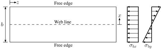
(a) Axial stresses due to bending

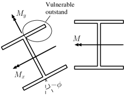
(b) Bending moments under LTB

Figure 2: After LTB: (a) top flange stress components from strong ($\sigma_{bx}$) and weak axis ($\sigma_{by}$) bending moments; (b) induced bending moment components during LTB, $M_{x}$ and $M_{y}$, which force one of the flange outstands to become more heavily compressed and hence vulnerable to local buckling.

shows a plan view of the top flange of the beam and the stress distribution components from the strong axis and the induced weak axis bending moments. Therefore, the maximum strong axis compressive stress occurs when $y=h/2$ and coupling this with the co-existing compressive component of the weak axis stress, the most vulnerable flange outstand is defined, as shown in Figure 2(b). Since the important component of bending under LTB is about the weak axis, the values of the relevant second moment of area for the flange ($I_{f}$) can be approximated to $I_{y}/2$ of the whole section, where $I_{y}=b^{3}t_{f}/6$, by assuming that the overall contribution of the web is very small, which is true for I-beams of practical dimensions. The strain energy stored in the beam due to bending ($U_{b}$) is therefore:

$$U_{b}=\frac{1}{2}EI_{f}\int_{0}^{L}\left(u_{t}^{\prime\prime 2}+u_{b}^{\prime\prime 2}\right)\mbox{$\,\mathrm{d}$}z=\frac{1}{2}EI_{y}\int_{0}^{L}u_{s}^{\prime\prime 2}\mbox{$\,\mathrm{d}$}z+\frac{1}{2}EI_{w}\int_{0}^{L}\phi^{\prime\prime 2}\mbox{$\,\mathrm{d}$}z,$$ (3)

where primes denote differentiation with respect to the axial coordinate $z$, $u_{w}=h\phi/2$ and $I_{w}=I_{y}h^{2}/4$. The strain energy stored from uniform torsion ($U_{T}$) is:

$$U_{T}=\frac{1}{2}\int_{0}^{L}T\mbox{$\,\mathrm{d}$}\phi=\frac{1}{2}GJ\int_{0}^{L}\phi^{\prime 2}\mbox{$\,\mathrm{d}$}z,$$ (4)

where $T$ is the torque, $G$ is the material shear modulus and $J$ is the St Venant torsion constant defined for an I-section as:

$$J=\frac{1}{3}\left[2bt_{f}^{3}+(h-2t_{f})t_{w}^{3}\right].$$ (5)

The work done by the external moment $M\Theta$ is given by the induced weak axis moment $M_{y}$ multiplied by the average end rotation from bending about the weak axis; this is given by the following expression [21]:

$$M\Theta=\int_{0}^{L}M\phi u_{s}^{\prime\prime}\mbox{$\,\mathrm{d}$}z$$ (6)

and so the total potential energy is thus:

$$V=U_{b}+U_{T}-M\Theta=\int_{0}^{L}\left[\frac{1}{2}EI_{y}u_{s}^{\prime\prime 2}+\frac{1}{2}EI_{w}\phi^{\prime\prime 2}+\frac{1}{2}GJ\phi^{\prime 2}-M\phi u_{s}^{\prime\prime}\right]\mbox{$\mathrm{d}$}z.$$ (7)

To find the critical moment $M_{\mathrm{cr}}$, the calculus of variations could be used to derive the governing differential equation. However, since the solution of the buckling mode is known to be sinusoidal [4], the same result can be achieved by using a two degree of freedom Rayleigh–Ritz formulation with the following trial functions:

$$u_{s}=q_{s}L\sin\frac{\pi z}{L},\quad\phi=-q_{\phi}\sin\frac{\pi z}{L},$$ (8)

where $q_{s}$ and $q_{\phi}$ are generalized coordinates defining the amplitudes of $u_{s}$ and $\phi$ respectively. Note that owing to the coordinate system used, the negative sign in front of $q_{\phi}$ is necessary to ensure that $q_{\phi}>0$ when $q_{s}>0$. Substituting the expressions for $u_{s}$ and $\phi$ from Equation (8) gives:

$$V=\int_{0}^{L}\left[\frac{EI_{y}\pi^{4}}{2L^{2}}\sin^{2}\frac{\pi z}{L}\left(q_{s}^{2}+q_{\phi}^{2}\lambda^{2}\right)+\frac{GJ\pi^{2}}{2L^{2}}q_{\phi}^{2}\cos^{2}\frac{\pi z}{L}-\frac{M}{L}q_{s}q_{\phi}\pi^{2}\sin^{2}\frac{\pi z}{L}\right]\mbox{$\mathrm{d}$}z$$ (9)

where $\lambda=h/2L$. The formulation is in small deflections (linear) and so only a critical equilibrium analysis is possible at this stage. The advantage of using the Rayleigh–Ritz method becomes more apparent in the interactive buckling model below. Performing the integration and then assembling the Hessian matrix $\mathbf{V}_{ij}$ at the critical point $\mathrm{C}$, gives the following condition:

$$\mathbf{V}_{ij}^{\mathrm{C}}=\left|\begin{array}[]{cc}V^{\mathrm{C}}_{ss}&V^{\mathrm{C}}_{s\phi}\\ V^{\mathrm{C}}_{\phi s}&V^{\mathrm{C}}_{\phi\phi}\end{array}\right|=\left|\begin{array}[]{cc}EI_{y}(\pi/L)^{4}&-\mbox{$M_{\mathrm{cr}}$}(\pi/L)^{2}\\ -\mbox{$M_{\mathrm{cr}}$}(\pi/L)^{2}&GJ(\pi/L)^{2}+EI_{w}(\pi/L)^{4}\\ \end{array}\right|=0,$$ (10)

where the individual elements of the matrix $\mathbf{V}_{ij}^{\mathrm{C}}$ are thus:

$$V_{ab}^{\mathrm{C}}=\left.\frac{\partial^{2}V}{\partial q_{a}\partial q_{b}}\right|^{\mathrm{C}}.$$ (11)

Solving equation (10) gives the classical expression for the critical moment $M_{\mathrm{cr}}$ that triggers LTB for a beam with a doubly-symmetric cross-section under uniform bending [4]:

$$\mbox{$M_{\mathrm{cr}}$}=\frac{\pi}{L}\sqrt{EI_{y}GJ}\sqrt{1+\frac{\pi^{2}}{L^{2}}\frac{EI_{w}}{GJ}}.$$ (12)

2.2 Interactive buckling model

From the previous section, it has been shown that as the displacements and rotations from LTB grow the applied moment $M$ can be expressed as a component about the strong axis ($M_{x}$) and an induced component about the weak axis ($M_{y}$) at any point along $z$. As a result, the vulnerable outstand of the flange, as identified in Figure 2, may therefore buckle locally as a plate. The critical stress of plate buckling for a uniaxially and uniformly compressed rectangular plate, with one long edge pinned and the other free, is given by the well known formula [4]:

$$\sigma^{\mathrm{C}}_{\mathrm{Local}}=0.43\frac{\pi^{2}D}{b_{f}^{2}t_{f}},$$ (13)

where, in the current case, $b_{f}$ is the width of the vulnerable flange outstand and is given by $(b-t_{w})/2$ and $D$ is the flexural rigidity of the flange plate that is equal to $Et_{f}^{3}/[12(1-\nu^{2})]$. This addresses the case for the flange buckling locally before any LTB occurs.

It was shown in [6] that the intrinsic assumptions in Euler–Bernoulli bending theory were insufficient to model any interaction between global and local buckling modes. The allowance of shear strains to develop within the individual elements, however small, being key to the formulation. Figure 3

(a) Top flange

(b) Bottom flange

Figure 3: Sway (upper row) and tilt (lower row) modes of LTB in both flanges.

shows a useful way that shear can be introduced; the displacement of the top and bottom flanges being decomposed into separate “sway” and “tilt” modes [22] after the global instability (LTB) has been triggered. Each original generalized coordinate $q_{s}$ and $q_{\phi}$ is defined as a “sway” and has a corresponding “tilt” component, with associated generalized coordinates $q_{t}$ and $q_{\tau}$ respectively. This is akin to a Timoshenko beam formulation [23]; when $q_{s}\neq q_{t}$ and $q_{\phi}\neq q_{\tau}$, shear strains are developed and allow the potential for modelling simultaneous LTB and local buckling.

Previous work on this type of interactive buckling has included experimental work combined with effective width theory [10], some phenomenological modelling using rigid links and springs along with experiments [11], some numerical work using a finite strip formulation [12, 13] and a finite element formulation [24]. To model this analytically, however, two displacement functions to account for the extra in-plane displacement $u$ and out-of-plane displacement $w$ (Figure 4)

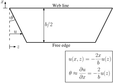
(a) $u(x,z)$

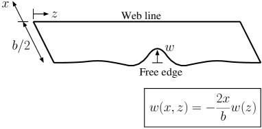
(b) $w(x,z)$

Figure 4: Displacement functions $u$ and $w$ defined for the vulnerable part of the top flange: $x=[-b/2,0]$ and $y=[h/2-t_{f},h/2]$.

need to be defined. Since the strain from the weak axis moment is linear in $x$ and that the boundary condition for the line of the web is pinned out of the plane of the flange, the following linear distribution in $x$ can be assumed for $u$ and $w$:

$$u(x,z)=-\frac{2x}{b}u(z),\quad w(x,z)=-\frac{2x}{b}w(z).$$ (14)

It is worth noting that restricting both interactive buckling displacement functions $u$ and $w$ to the vulnerable part of the compression flange confines the current model to cases where LTB occurs before local buckling. In the cases where local buckling occurs first, the system would be expected to trigger the global mode rapidly afterwards [25] and the current model can be used to indicate the deformation levels where the interaction would occur (as seen later). However, to obtain an accurate linear eigenvalue solution for pure local buckling in the current framework, at least another set of in-plane and out-of-plane displacement functions, replicating the role of $u$ and $w$ respectively, would need to be defined for the non-vulnerable part of the compression flange; this addition is left for future work.

2.2.1 Local bending energy

Experimental evidence, presented in [24], suggests that during interactive buckling the significant local out-of-plane displacements within the flanges are confined to the vulnerable outstand. The component of additional strain energy stored in bending $U_{bl}$ is hence given by:

$$U_{bl}=\frac{D}{2}\int_{0}^{L}\int_{-b/2}^{0}\left\{\left(\frac{\partial^{2}w}{\partial x^{2}}+\frac{\partial^{2}w}{\partial z^{2}}\right)^{2}-2(1-\nu)\left[\frac{\partial^{2}w}{\partial x^{2}}\frac{\partial^{2}w}{\partial z^{2}}-\left(\frac{\partial^{2}w}{\partial x\partial z}\right)^{2}\right]\right\}\,\mathrm{d}x\,\mathrm{d}z.$$ (15)

Substituting $w$ into $U_{bl}$, the following expression is obtained:

$$U_{bl}=\frac{D}{2b}\int_{0}^{L}\left[\frac{b^{2}}{6}w^{\prime\prime 2}+4(1-\nu)w^{\prime 2}\right]\,\mathrm{d}z.$$ (16)

2.2.2 Flange energy from axial and shear strains

Since the flanges are assumed to behave in the manner of Timoshenko beams, the bending of the flanges when LTB occurs introduce both axial and shear strains, $\varepsilon$ and $\gamma$ respectively. The vulnerable part of the top flange, where $x=[-b/2,0]$ and $y=[h/2-t_{f},h/2]$, also has the possibility of local buckling; von Kármán plate theory gives a standard expression for the axial strain $\varepsilon$ in the $z$-direction that accounts for both LTB and local buckling terms, thus:

$$\varepsilon_{t1}=\frac{\partial u_{tt}}{\partial z}+\frac{\partial u}{\partial z}+\frac{1}{2}\left(\frac{\partial w}{\partial z}\right)^{2}=(q_{t}+q_{\tau}\lambda)\frac{\pi^{2}x}{L}\sin\frac{\pi z}{L}-\frac{2x}{b}u^{\prime}+\frac{2x^{2}}{b^{2}}w^{\prime 2}.$$ (17)

For the part of the top flange that is not vulnerable to local buckling, where $x=[0,b/2]$ and $y=[h/2-t_{f},h/2]$, and the bottom flange, where $y=[-h/2,-h/2+t_{f}]$, the following respective axial strain expressions are obtained:

$$\varepsilon_{t2} =\frac{\partial u_{tt}}{\partial z}=(q_{t}+q_{\tau}\lambda)\frac{\pi^{2}x}{L}\sin\frac{\pi z}{L},$$ (18)

$$\varepsilon_{b} =\frac{\partial u_{tb}}{\partial z}=(q_{t}-q_{\tau}\lambda)\frac{\pi^{2}x}{L}\sin\frac{\pi z}{L}.$$ (19)

The standard strain energy expression is then integrated over the volume of the flanges:

$$\begin{split}U_{m}&=\frac{E}{2}\int_{0}^{L}\left[\int_{h/2-t_{f}}^{h/2}\int_{-b/2}^{0}\varepsilon_{t1}^{2}\mbox{$\,\mathrm{d}$}x\mbox{$\,\mathrm{d}$}y+\int_{h/2-t_{f}}^{h/2}\int_{0}^{b/2}\varepsilon_{t2}^{2}\mbox{$\,\mathrm{d}$}x\mbox{$\,\mathrm{d}$}y+\int_{-h/2}^{-h/2+t_{f}}\int_{-b/2}^{b/2}\varepsilon_{b}^{2}\mbox{$\,\mathrm{d}$}x\mbox{$\,\mathrm{d}$}y\right]\mbox{$\mathrm{d}$}z\\ &=\frac{Ebt_{f}}{12}\int_{0}^{L}\biggl{[}u^{\prime 2}+\frac{3}{20}w^{\prime 4}+\frac{3}{4}u^{\prime}w^{\prime 2}-(q_{t}+q_{\tau}\lambda)\pi^{2}\psi\sin\frac{\pi z}{L}\left(u^{\prime}+\frac{3}{8}w^{\prime 2}\right)\\ &\qquad\qquad\qquad+\left(q_{t}^{2}+q_{\tau}^{2}\lambda^{2}\right)\pi^{4}\psi^{2}\sin^{2}\frac{\pi z}{L}\biggr{]}\mbox{$\,\mathrm{d}$}z,\end{split}$$ (20)

where $\psi=b/L$ is a beam aspect ratio parameter. It is worth noting that the transverse displacement and the strain in the $x$-direction are omitted from the current formulation. This is a simplification derived from [7], where these components were found to have a negligible effect on the post-buckling stiffness of a uniaxially compressed long plate with one longitudinal edge being pinned and the other being free.

In terms of the shear strain $\gamma$ in the $xz$ plane within the top flange, where $y=[h/2-t_{f},h/2]$, von Kármán plate theory gives a standard expression, which needs to account for both LTB and local terms for the vulnerable outstand $x=[-b/2,0]$:

$$\begin{split}\gamma_{t1}&=\theta_{st}-\theta_{tt}+\text{local buckling terms}\\ &=\frac{\partial u_{st}}{\partial z}+\frac{\partial u_{tt}}{\partial x}+\frac{\partial u}{\partial x}+\frac{\partial w}{\partial x}\frac{\partial w}{\partial z}=\left[(q_{s}-q_{t})+(q_{\phi}-q_{\tau})\lambda\right]\pi\cos\frac{\pi z}{L}-\frac{2}{b}u+\frac{4x}{b^{2}}ww^{\prime},\end{split}$$ (21)

and purely LTB terms for the non-vulnerable part of the top flange, $x=[0,b/2]$, and the bottom flange, where $y=[-h/2,-h/2+t_{f}]$, respectively:

$$\gamma_{t2} =\theta_{st}-\theta_{tt}=\frac{\partial u_{st}}{\partial z}+\frac{\partial u_{tt}}{\partial x}=\left[(q_{s}-q_{t})+(q_{\phi}-q_{\tau})\lambda\right]\pi\cos\frac{\pi z}{L},$$ (22)

$$\gamma_{b} =\theta_{sb}-\theta_{tb}=\frac{\partial u_{sb}}{\partial z}+\frac{\partial u_{tb}}{\partial x}=\left[(q_{s}-q_{t})-(q_{\phi}-q_{\tau})\lambda\right]\pi\cos\frac{\pi z}{L}.$$ (23)

After obtaining the shear strains, the standard strain energy expression needs to be integrated over the volume of the flanges, thus:

$$\begin{split}U_{s}&=\frac{G}{2}\int_{0}^{L}\left[\int_{h/2-t_{f}}^{h/2}\int_{-b/2}^{0}\gamma_{t1}^{2}\mbox{$\,\mathrm{d}$}x\mbox{$\,\mathrm{d}$}y+\int_{h/2-t_{f}}^{h/2}\int_{0}^{b/2}\gamma_{t2}^{2}\mbox{$\,\mathrm{d}$}x\mbox{$\,\mathrm{d}$}y+\int_{-h/2}^{-h/2+t_{f}}\int_{-b/2}^{b/2}\gamma_{b}^{2}\mbox{$\,\mathrm{d}$}x\mbox{$\,\mathrm{d}$}y\right]\mbox{$\mathrm{d}$}z\\ &=\frac{Gbt_{f}}{2}\int_{0}^{L}\biggl{\{}\frac{2}{b^{2}}\left(u^{2}+\frac{1}{3}w^{2}w^{\prime 2}+uww^{\prime}\right)-\left[(q_{s}-q_{t})+(q_{\phi}-q_{\tau})\lambda\right]\frac{\pi}{b}\cos\frac{\pi z}{L}\left(2u+ww^{\prime}\right)\\ &\qquad\qquad\qquad+\left[(q_{s}-q_{t})^{2}+(q_{\phi}-q_{\tau})^{2}\lambda^{2}\right]2\pi^{2}\cos^{2}\frac{\pi z}{L}\biggr{\}}\mbox{$\,\mathrm{d}$}z.\end{split}$$ (24)

2.2.3 Work done contribution

An additional contribution from the vulnerable flange’s local in-plane displacement function $u$ needs to be included in the work done term. Figure 5

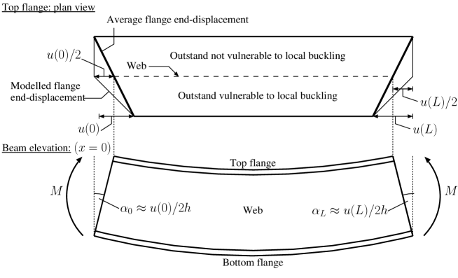
Figure 5: Contribution from local buckling in the work done term, where $h$ is the overall cross-section height.

shows that the compression flange has a distribution of in-plane displacement which is assumed to have an average linear distribution in $x$. Including this as an average end-rotation, angles $\alpha_{0}$ and $\alpha_{L}$ are obtained as shown in the diagram. Since the end rotation angles can be expressed in terms of the local in-plane displacement function $u$, the expression for the local contribution to the work done is:

$$M\Theta_{l}=M_{x}(\alpha_{0}-\alpha_{L})=-\frac{M}{2h}\int_{0}^{L}u^{\prime}\mbox{$\,\mathrm{d}$}z.$$ (25)

2.2.4 Total potential energy

The expression for the total potential energy of the interactive buckling model system can be written as a sum of the individual terms of the strain energies minus the work done terms from §2.1 and §2.2, with $U_{m}$ and $U_{s}$ replacing $U_{b}$ to account for the change in the bending theory assumptions:

$$\begin{split}V=U_{m}+U_{T}+U_{bl}+U_{s}-M(\Theta+\Theta_{l}).\end{split}$$ (26)

This new energy function $V$ replaces equation (7) and is written in terms of non-dimensionalized variables that replace the original ones, thus:

$$\tilde{u}=\frac{2}{L}u,\quad\tilde{w}=\frac{2}{L}w,\quad\tilde{z}=\frac{2}{L}z,$$ (27)

giving the full expression for $V$, where primes henceforth represent derivatives with respect to $\tilde{z}$:

$$\begin{split}V=\frac{L}{2}\int_{0}^{2}&\biggr{\{}\frac{Ebt_{f}}{12}\biggl{[}\mbox{$\tilde{u}$}^{\prime 2}+\frac{3}{20}\mbox{$\tilde{w}$}^{\prime 4}+\frac{3}{4}\mbox{$\tilde{u}$}^{\prime}\mbox{$\tilde{w}$}^{\prime 2}-(q_{t}+q_{\tau}\lambda)\pi^{2}\psi\sin\frac{\pi\mbox{$\tilde{z}$}}{2}\left(\mbox{$\tilde{u}$}^{\prime}+\frac{3}{8}\mbox{$\tilde{w}$}^{\prime 2}\right)\\ &+\left(q_{t}^{2}+q_{\tau}^{2}\lambda^{2}\right)\pi^{4}\psi^{2}\sin^{2}\frac{\pi\mbox{$\tilde{z}$}}{2}\biggr{]}+\frac{GJ\pi^{2}}{2L^{2}}q_{\phi}^{2}\cos^{2}\frac{\pi\mbox{$\tilde{z}$}}{2}+\frac{D}{b}\left[\frac{\psi^{2}}{3}\mbox{$\tilde{w}$}^{\prime\prime 2}+2(1-\nu)\mbox{$\tilde{w}$}^{\prime 2}\right]\\ &+\frac{Gbt_{f}}{2}\biggl{[}\frac{1}{2\psi^{2}}\left(u^{2}+\frac{1}{3}\mbox{$\tilde{w}$}^{2}\mbox{$\tilde{w}$}^{\prime 2}+\mbox{$\tilde{u}$}\mbox{$\tilde{w}$}\mbox{$\tilde{w}$}^{\prime}\right)+\left[(q_{s}-q_{t})^{2}+(q_{\phi}-q_{\tau})^{2}\lambda^{2}\right]2\pi^{2}\cos^{2}\frac{\pi\mbox{$\tilde{z}$}}{2}\\ &-\left[(q_{s}-q_{t})+(q_{\phi}-q_{\tau})\lambda\right]\frac{\pi}{\psi}\cos\frac{\pi\mbox{$\tilde{z}$}}{2}\left(\mbox{$\tilde{u}$}+\frac{1}{2}\mbox{$\tilde{w}$}\mbox{$\tilde{w}$}^{\prime}\right)\biggr{]}-\frac{M}{L}\left(q_{s}q_{\phi}\pi^{2}\sin^{2}\frac{\pi\mbox{$\tilde{z}$}}{2}-\frac{1}{4\lambda}\mbox{$\tilde{u}$}^{\prime}\right)\biggr{\}}\mbox{$\mathrm{d}$}\mbox{$\tilde{z}$}.\end{split}$$ (28)

2.2.5 Linear eigenvalue analysis

With $u$ and $w$ being zero, along with their derivatives, before any local buckling occurs, the Hessian matrix $\mathbf{V}_{ij}$, now including terms associated with the “tilt” generalized coordinates, can still be used to find $M_{\mathrm{cr}}$ the critical moment for LTB. The Hessian matrix is thus:

$$\mathbf{V}_{ij}^{\mathrm{F}}=\left(\begin{array}[]{cccc}V_{ss}&V_{st}&V_{s\phi}&V_{s\tau}\\ V_{ts}&V_{tt}&V_{t\phi}&V_{t\tau}\\ V_{\phi s}&V_{\phi t}&V_{\phi\phi}&V_{\phi\tau}\\ V_{\tau s}&V_{\tau t}&V_{\tau\phi}&V_{\tau\tau}\end{array}\right),$$ (29)

with the individual terms being:

$$\begin{split}V_{ss}&=GLbt_{f}\pi^{2},\quad V_{tt}=\frac{EI_{y}\pi^{4}\psi^{2}}{2L}+GLbt_{f}\pi^{2},\quad V_{\phi\phi}=\frac{GJ\pi^{2}}{2L}+GLbt_{f}\pi^{2},\\ V_{\tau\tau}&=\frac{EI_{w}\pi^{4}}{2L^{3}}+GLbt_{f}\pi^{2}\lambda^{2}=\pi^{2}\lambda^{2}\left(\frac{EI_{y}\pi^{2}}{2L}+GLbt_{f}\right),\quad V_{st}=V_{ts}=-GLbt_{f}\pi^{2},\\ V_{s\phi}&=V_{\phi s}=-\frac{M\pi^{2}}{2},\quad V_{\phi\tau}=V_{\tau\phi}=-GLbt_{f}\pi^{2}\lambda^{2},\quad V_{s\tau}=V_{\tau s}=V_{t\tau}=V_{\tau t}=V_{t\phi}=V_{\phi t}=0,\end{split}$$ (30)

which when substituted into $\mathbf{V}_{ij}$ with the singular condition at the critical point $\mathrm{C}$, where $M=\mbox{$M_{\mathrm{cr}}$}$, gives:

$$\mbox{$M_{\mathrm{cr}}$}=\frac{\pi}{L}\sqrt{\frac{EI_{y}GJ}{1+s}}\sqrt{1+\frac{1}{(1+s)}\frac{\pi^{2}}{L^{2}}\frac{EI_{w}}{GJ}}.$$ (31)

This new expression for $M_{\mathrm{cr}}$ replaces equation (12) and is used subsequently. The term, $s=E\pi^{2}\psi^{2}/12G$, accounts for the non-zero shear distortion of both flanges, which tends to zero if $G$ or $L$ become large; this is an entirely logical result reflecting the difference between Timoshenko and Euler–Bernoulli beam theories [23]. However with $s>0$, the above expression gives values that are marginally below those given by the classical critical moment given in equation (12).

2.2.6 Equilibrium equations

The total potential energy $V$ with the rescaled variables can be written thus:

$$V=\int_{0}^{2}\mathcal{L}(\mbox{$\tilde{w}$}^{\prime\prime},\mbox{$\tilde{w}$}^{\prime},\mbox{$\tilde{w}$},\mbox{$\tilde{u}$}^{\prime},\mbox{$\tilde{u}$};\mbox{$\tilde{z}$})\mbox{$\,\mathrm{d}$}\mbox{$\tilde{z}$}.$$ (32)

Equilibrium equations are found where $V$ is stationary and this is established from setting the first variation of $V$ (or $\delta V$) to zero, where:

$$\begin{split}\delta V&=\int_{0}^{2}\left[\frac{\partial\mathcal{L}}{\partial\mbox{$\tilde{w}$}^{\prime\prime}}\delta\mbox{$\tilde{w}$}^{\prime\prime}+\frac{\partial\mathcal{L}}{\partial\mbox{$\tilde{w}$}^{\prime}}\delta\mbox{$\tilde{w}$}^{\prime}+\frac{\partial\mathcal{L}}{\partial\mbox{$\tilde{w}$}}\delta\mbox{$\tilde{w}$}+\frac{\partial\mathcal{L}}{\partial\mbox{$\tilde{u}$}^{\prime}}\delta\mbox{$\tilde{u}$}^{\prime}+\frac{\partial\mathcal{L}}{\partial\mbox{$\tilde{u}$}}\delta\mbox{$\tilde{u}$}\right]\mbox{$\,\mathrm{d}$}\mbox{$\tilde{z}$}\\ &=\left\{\frac{\partial\mathcal{L}}{\partial\mbox{$\tilde{w}$}^{\prime\prime}}\delta\mbox{$\tilde{w}$}^{\prime}+\left[\frac{\partial\mathcal{L}}{\partial\mbox{$\tilde{w}$}^{\prime}}-\frac{\mbox{$\mathrm{d}$}}{\mbox{$\mathrm{d}$}\mbox{$\tilde{z}$}}\left(\frac{\partial\mathcal{L}}{\partial\mbox{$\tilde{w}$}^{\prime\prime}}\right)\right]\delta\mbox{$\tilde{w}$}+\frac{\partial\mathcal{L}}{\partial\mbox{$\tilde{u}$}^{\prime}}\delta\mbox{$\tilde{u}$}\right\}_{0}^{2}\\ &\qquad+\int_{0}^{2}\left\{\left[\frac{\mbox{$\mathrm{d}$}^{2}}{\mbox{$\mathrm{d}$}\mbox{$\tilde{z}$}^{2}}\left(\frac{\partial\mathcal{L}}{\partial\mbox{$\tilde{w}$}^{\prime\prime}}\right)-\frac{\mbox{$\mathrm{d}$}}{\mbox{$\mathrm{d}$}\mbox{$\tilde{z}$}}\left(\frac{\partial\mathcal{L}}{\partial\mbox{$\tilde{w}$}^{\prime}}\right)+\frac{\partial\mathcal{L}}{\partial\mbox{$\tilde{w}$}}\right]\delta\mbox{$\tilde{w}$}+\left[\frac{\partial\mathcal{L}}{\partial\mbox{$\tilde{u}$}}-\frac{\mbox{$\mathrm{d}$}}{\mbox{$\mathrm{d}$}\mbox{$\tilde{z}$}}\left(\frac{\partial\mathcal{L}}{\partial\mbox{$\tilde{u}$}^{\prime}}\right)\right]\delta\mbox{$\tilde{u}$}\right\}\mbox{$\,\mathrm{d}$}\mbox{$\tilde{z}$}.\end{split}$$ (33)

The term in the integral has to vanish for all $\delta w$ and $\delta u$, which gives two coupled nonlinear ordinary differential equations:

$$\begin{split}&\mbox{$\tilde{w}$}^{\prime\prime\prime\prime}-\frac{6(1-\nu)}{\psi^{2}}\mbox{$\tilde{w}$}^{\prime\prime}-\frac{3GL^{2}t_{f}}{8D\psi^{2}}\mbox{$\tilde{w}$}\left[\mbox{$\tilde{u}$}^{\prime}+\frac{2}{3}(\mbox{$\tilde{w}$}^{\prime 2}+\mbox{$\tilde{w}$}\mbox{$\tilde{w}$}^{\prime\prime})+\left[q_{s}-q_{t}+\lambda(q_{\phi}-q_{\tau})\right]\frac{\pi^{2}\psi}{2}\sin\frac{\pi\mbox{$\tilde{z}$}}{2}\right]\\ &\quad+\frac{3EL^{2}t_{f}}{8D}\biggl{[}(q_{t}+q_{\tau}\lambda)\frac{\pi^{2}\psi}{4}\left(\sin\frac{\pi\mbox{$\tilde{z}$}}{2}\mbox{$\tilde{w}$}^{\prime\prime}+\frac{\pi}{2}\cos\frac{\pi\mbox{$\tilde{z}$}}{2}\mbox{$\tilde{w}$}^{\prime}\right)-\frac{1}{2}(\mbox{$\tilde{u}$}^{\prime\prime}\mbox{$\tilde{w}$}^{\prime}+\mbox{$\tilde{u}$}^{\prime}\mbox{$\tilde{w}$}^{\prime\prime})-\frac{3}{5}\mbox{$\tilde{w}$}^{\prime 2}\mbox{$\tilde{w}$}^{\prime\prime}\biggr{]}=0,\end{split}$$ (34)

$$\mbox{$\tilde{u}$}^{\prime\prime}+\frac{3}{4}\mbox{$\tilde{w}$}^{\prime}\mbox{$\tilde{w}$}^{\prime\prime}+\frac{\pi^{2}}{4s}\left\{\pi\psi\cos\frac{\pi z}{2}\left[\left(q_{s}-q_{t}+\lambda(q_{\phi}-q_{\tau})\right)-s(q_{t}+q_{\tau}\lambda)\right]-\left(\mbox{$\tilde{u}$}+\frac{1}{2}\mbox{$\tilde{w}$}\mbox{$\tilde{w}$}^{\prime}\right)\right\}=0,$$ (35)

subject to the following boundary conditions which arise from minimizing the terms outside the integral in equation (33):

$$\mbox{$\tilde{w}$}(0)=\mbox{$\tilde{w}$}^{\prime\prime}(0)=\mbox{$\tilde{w}$}(2)=\mbox{$\tilde{w}$}^{\prime\prime}(2) =0,$$ (36)

$$\mbox{$\tilde{u}$}^{\prime}(0)+\frac{3}{8}\mbox{$\tilde{w}$}^{\prime 2}(0)+\frac{3M}{Ebht_{f}} =0,$$ (37)

$$\mbox{$\tilde{u}$}(1)=\mbox{$\tilde{w}$}^{\prime}(1)=\mbox{$\tilde{w}$}^{\prime\prime\prime}(1) =0,$$ (38)

where equation (36) refers to pinned boundaries, equation (37) refers to the end strain condition, and equation (38) refers to reflective symmetry of $w$ and antisymmetry of $u$ about the midspan respectively. The symmetry conditions are particularly pertinent when LTB occurs simultaneously with or before local buckling owing to the sinusoidal distribution of $\phi$ forcing the maximum bending stress to be located at midspan.

Other equilibrium equations can be obtained by minimizing the energy with respect to the generalized coordinates $q_{s}$, $q_{\phi}$, $q_{t}$ and $q_{\tau}$:

$$\frac{\partial V}{\partial q_{s}} =\frac{G\pi^{2}Lbt_{f}}{4}\int_{0}^{2}\biggl{\{}\left[4(q_{s}-q_{t})\cos\frac{\pi\mbox{$\tilde{z}$}}{2}-\frac{1}{\pi\psi}\left(\mbox{$\tilde{u}$}+\frac{1}{2}\mbox{$\tilde{w}$}\mbox{$\tilde{w}$}^{\prime}\right)\right]\cos\frac{\pi\mbox{$\tilde{z}$}}{2}-\frac{2M}{GLbt_{f}}q_{\phi}\sin^{2}\frac{\pi\mbox{$\tilde{z}$}}{2}\biggr{\}}\mbox{$\,\mathrm{d}$}\mbox{$\tilde{z}$}=0,$$ (39)

$$\frac{\partial V}{\partial q_{\phi}} =\frac{G\pi^{2}bht_{f}}{2}\int_{0}^{2}\biggl{\{}\left[\left(\lambda(q_{\phi}-q_{\tau})+\frac{J}{Lbht_{f}}q_{\phi}\right)\cos\frac{\pi\mbox{$\tilde{z}$}}{2}-\frac{1}{4\pi\psi}\left(\mbox{$\tilde{u}$}+\frac{1}{2}\mbox{$\tilde{w}$}\mbox{$\tilde{w}$}^{\prime}\right)\right]\cos\frac{\pi\mbox{$\tilde{z}$}}{2}$$ (40)

$$\qquad\qquad\qquad\qquad-\frac{M}{Gbht_{f}}q_{s}\sin^{2}\frac{\pi\mbox{$\tilde{z}$}}{2}\biggr{\}}\mbox{$\,\mathrm{d}$}\mbox{$\tilde{z}$}=0,$$

$$\frac{\partial V}{\partial q_{t}} =\frac{E\pi^{2}Lbt_{f}}{4}\int_{0}^{2}\biggl{\{}\left[2q_{t}\pi^{2}\psi\sin\frac{\pi\mbox{$\tilde{z}$}}{2}-\left(\mbox{$\tilde{u}$}^{\prime}+\frac{3}{8}\mbox{$\tilde{w}$}^{\prime 2}\right)\right]\frac{\psi}{6}\sin\frac{\pi\mbox{$\tilde{z}$}}{2}$$ (41)

$$\qquad\qquad\qquad\qquad+\left[\frac{1}{\pi\psi}\left(\mbox{$\tilde{u}$}+\frac{1}{2}\mbox{$\tilde{w}$}\mbox{$\tilde{w}$}^{\prime}\right)-4(q_{s}-q_{t})\cos\frac{\pi\mbox{$\tilde{z}$}}{2}\right]\frac{G}{E}\cos\frac{\pi\mbox{$\tilde{z}$}}{2}\biggr{\}}\mbox{$\,\mathrm{d}$}\mbox{$\tilde{z}$}=0,$$

$$\frac{\partial V}{\partial q_{\tau}} =\frac{E\pi^{2}bht_{f}}{8}\int_{0}^{2}\biggl{\{}\left[2q_{\tau}\lambda\pi^{2}\psi\sin\frac{\pi\mbox{$\tilde{z}$}}{2}-\left(\mbox{$\tilde{u}$}^{\prime}+\frac{3}{8}\mbox{$\tilde{w}$}^{\prime 2}\right)\right]\frac{\psi}{6}\sin\frac{\pi\mbox{$\tilde{z}$}}{2}$$ (42)

$$\qquad\qquad\qquad\qquad+\left[\frac{1}{\pi\psi}\left(\mbox{$\tilde{u}$}+\frac{1}{2}\mbox{$\tilde{w}$}\mbox{$\tilde{w}$}^{\prime}\right)-4\lambda(q_{\phi}-q_{\tau})\cos\frac{\pi\mbox{$\tilde{z}$}}{2}\right]\frac{G}{E}\cos\frac{\pi\mbox{$\tilde{z}$}}{2}\biggr{\}}\mbox{$\mathrm{d}$}\mbox{$\tilde{z}$}=0.$$

3 Physical experiments

3.1 Specimens and procedure

A series of physical experiments were conducted on I-beams fabricated by spot-welding thin-walled channel sections, made from cold-formed steel, back-to-back. The key material properties were measured to be thus: Young’s modulus $E=205~{}\mathrm{kN/mm^{2}}$, Poisson’s ratio $\nu=0.3$ and the yield stress $\sigma_{\mathrm{y}}=290~{}\mathrm{N/mm^{2}}$. The channel sections were $75\times 43\times 2~{}\mbox{$\mathrm{mm}$}$ in terms of depth, width and thickness respectively – see Figure 6(a).

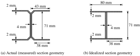
Figure 6: Cross-section of steel beams tested in the experimental programme. (a) Actual section constructed from two channel sections; (b) idealized section geometry derived from experiments.

The actual geometry (including corner radii etc.) was converted into an idealized I-section comprising only flat plate elements based on the mean slope of the linear regions of the measured load versus maximum bending displacement curves from the tests. The dimensions of $h$ and $b$ were hence adjusted slightly such that a meaningful comparison with the theory could be made – see Figure 6(b). Each beam, the idealized properties of which are given in Table 1,

Geometric Property	Value	Cross-Section Property	Value
$b$	$80~{}\mbox{$\mathrm{mm}$}$	$I_{x}$	$4.81\times 10^{5}~{}\mbox{$\mathrm{mm}$}^{4}$
$h$	$71~{}\mbox{$\mathrm{mm}$}$	$I_{y}$	$1.71\times 10^{5}~{}\mbox{$\mathrm{mm}$}^{4}$
$t_{f}$	$2~{}\mbox{$\mathrm{mm}$}$	$I_{w}$	$2.16\times 10^{8}~{}\mbox{$\mathrm{mm}$}^{6}$
$t_{w}$	$4~{}\mbox{$\mathrm{mm}$}$	$J$	$1.86\times 10^{3}~{}\mbox{$\mathrm{mm}$}^{4}$

Table 1: Idealized section properties of the experimental samples.

had an overall length of 4 metres, was tested under four-point bending with a specified buckling length $L_{e}$ given in Table 2

Test	Effective length $L_{e}~{}(\mbox{$\mathrm{mm}$})$	$\sigma^{\mathrm{C}}_{\mathrm{Local}}/\sigma^{\mathrm{C}}_{\mathrm{LTB}}$	$\sigma^{\mathrm{C}}~{}(\mathrm{N/mm^{2}})$	Critical mode
$1$	$3200$	1.19	186	LTB
$2$	$3200$	1.19	186	LTB
$3$	$3000$	1.10	202	LTB
$4$	$2750$	0.98	221	Local (marginally)
$5$	$2500$	0.87	221	Local
$6$	$2250$	0.75	221	Local

Table 2: Buckling lengths for each beam test which reflect the symmetric position of the lateral restraints; these lengths were chosen such that $\sigma^{\mathrm{C}}_{\mathrm{Local}}/\sigma^{\mathrm{C}}_{\mathrm{LTB}}=[0.75,1.20]$ with one beam (Test 4) triggering both modes approximately simultaneously.

that was controlled by an adjustable pair of lateral restraints (see Figure 7 in §3.2). The critical mode was determined by comparing the strong axis bending stress when $M=\mbox{$M_{\mathrm{cr}}$}$, thus:

$$\sigma^{\mathrm{C}}_{\mathrm{LTB}}=\frac{\mbox{$M_{\mathrm{cr}}$}y_{\mathrm{max}}}{I_{x}}=\frac{\mbox{$M_{\mathrm{cr}}$}h}{2I_{x}},$$ (43)

with the critical stress of plate buckling being given by equation (13).

3.2 Testing rig

A schematic of the experimental setup along with an idealized representation is shown in Figure 7.

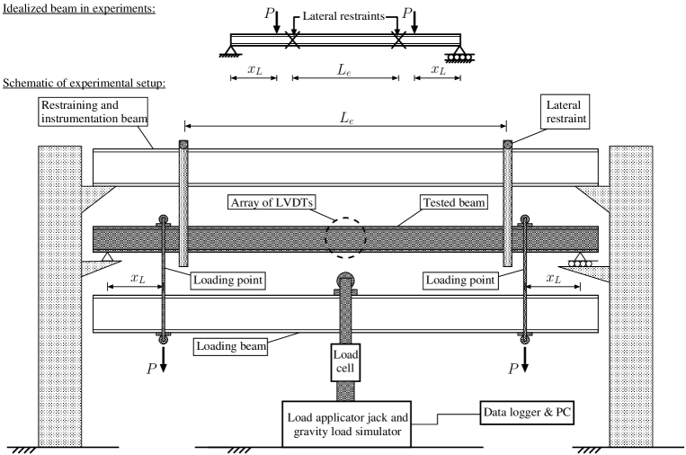
Figure 7: Experimental rig designed to test fabricated I-beams under four-point bending. Although each beam was $4~{}\mbox{$\mathrm{m}$}$ in length, the distance between the pinned supports was in fact $3.8~{}\mbox{$\mathrm{m}$}$. In each test, the lateral restraints were adjusted symmetrically to obtain the desired buckling length $L_{e}$.

The total applied load $2P$ was split into two point loads each of $P$ applied at a distance $x_{L}$ from the end supports. Hence, from simple statics, the uniform moment $M$ between the two loading points was $Px_{L}$. The loading was displacement controlled; it was applied with a hand-operated hydraulic jack in conjunction with a gravity load simulator, a mechanism that adjusted the position of the load application relative to the deflecting beam such that the applied load remained vertical. Since the jack was hand operated, the displacement was applied in short controlled increments but it did mean that dynamic loads were inevitable to a small extent. At midspan, the vertical displacement of the beam and lateral displacements of the flanges were measured using linear variable differential transformers (LVDTs); the locations of which are presented in Figure 8.

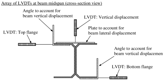
Figure 8: Cross-section of the tested beam showing the relative positions of the LVDTs. Angles and plates were clamped as shown to both flanges such that the overall beam displacement still allowed the relative flange and vertical displacements to be evaluated.

The large displacements and dynamic behaviour of unstable post-buckling, even with displacement control, meant that sometimes the LVDTs measuring the displacement of the greater displacing top flange – see Figure 1(b) – went out of range very quickly after the secondary instability was triggered. However, there were no such problems associated with the bottom flange measurements and so these were the primary values used for comparison purposes, since the theoretical model gives both $u_{s}$ and $\phi$ directly.

4 Numerical results and validation

4.1 Cellular buckling

The system of nonlinear ordinary differential equations (34)–(35), subject to boundary conditions from equations (36)–(38) and integral equations from (39)–(42) are solved using the well-known and tested numerical continuation package Auto [14]. For illustrative purposes, Figures 9–11

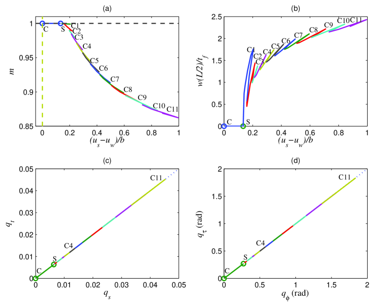
Figure 9: Numerical equilibrium paths for test specimen 1. Graphs of (a) normalized moment ratio $m$ and (b) local buckling displacement amplitude $w_{\mathrm{max}}/t_{f}$ versus lateral displacement of the bottom flange are shown. Points $\mathrm{C}$ and $\mathrm{S}$ show the critical and secondary bifurcation points respectively. Note that the sequence of paths, separated by snap-backs that mark the appearance of a new local buckling “cell”, are denoted as “$\mathrm{Cn}$” where $\mathrm{n}$ is the cell number. The graphs in (c) and (d) show the relationships between the generalized coordinates defining LTB during interactive buckling; note that the dotted lines represent the relationship between the respective quantities assuming Euler–Bernoulli bending, which show that the developed shear strains are small.

present results from the variational model for test specimen 1. Figure 9 shows a plot of the (a) normalized moment ratio $m$, which is defined as the ratio $M/\mbox{$M_{\mathrm{cr}}$}$, and (b) the normalized local buckling displacement amplitude ($w(L/2)/t_{f}$) of the vulnerable part of the compression flange versus the normalized lateral displacement of the bottom flange, $(u_{s}-u_{w})/b$. The graphs in (c) and (d) show the relationships between the “sway” and “tilt” components of the weak axis centroidal displacement ($q_{s}$ and $q_{t}$) and the torsional angle ($q_{\phi}$ and $q_{\tau}$). A dotted line is superimposed on these graphs to show the Euler–Bernoulli assumption, where the sway and tilt amplitudes would be equal; this shows that the shear strains developed are small but not zero. Moreover, Figures 9(a) and (b) show a series of paths separated by a sequence of snap-backs with Figure 10

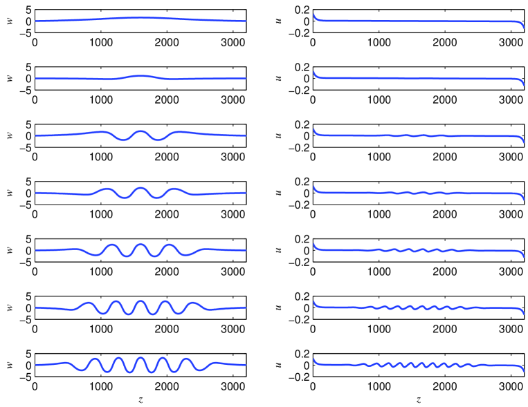
Figure 10: Numerical solutions of the displacements of local buckling for the tip ($x=-b/2$) of the vulnerable flange of test specimen 1: out-of plane displacement $w$ (left) and in-plane displacement $u$ (right). Individual solutions on equilibrium paths C1 to C7 (defined in Figure 9) are shown in sequence from top to bottom respectively. All dimensions are in millimetres.

presenting detailed graphs showing the corresponding numerical solutions beyond individual snap-backs for the local buckling functions. A distinctive pattern is clearly seen to emerge where the response passes from one path to the next, i.e. from C1 to C2 to C3 and so on, in which each new path reveals a new local buckling displacement peak or trough. A selection of 3-dimensional representations of the beams using the solutions for the paths C1, C3, C5 and C7 are presented in Figure 11,

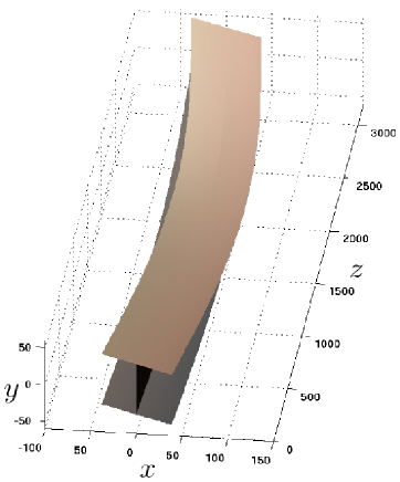
(a) C1: $m=0.9998$

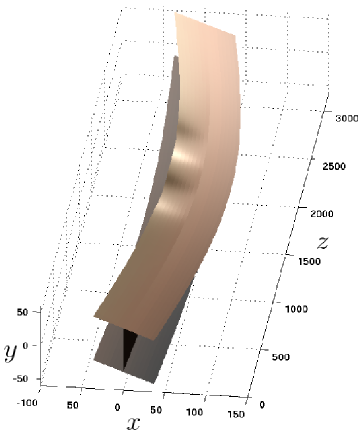
(b) C3: $m=0.9900$

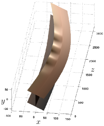
(c) C5: $m=0.9718$

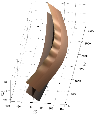
(d) C7: $m=0.9414$

Figure 11: Numerical solutions of the system of equilibrium equations visualized on a representation of the actual beam used in test 1. All deformation components: $w$, $u$, $u_{s}$, $\phi$, $u_{tb}$ and $u_{tt}$ are included with all dimensions in millimetres. The results are shown for individual points on paths C1, C3, C5 and C7 (Figure 9) with the specific moment ratio $m$ given. Note how the local buckling mode develops and how the “wavelength” of the local buckling profile within the central portion of the flange in more compression changes as more cells develop.

which include all components of LTB ($u_{s}$, $\phi$, $u_{tb}$ and $u_{tt}$) and local buckling ($w$ and $u$).

As the response advances to path C11, which has torsional rotations that are well beyond the scope of the model in terms of geometric considerations, the local buckle pattern is all but periodic and further loading would restabilize the system globally, assuming no permanent deformation has taken place. This global restabilization would occur as a result of the boundaries confining the spread of the buckling profile any further. Of course, if plasticity were present in the flange then any restabilization would be less significant and displacements would lock into plastic hinges.

The phenomenon demonstrated currently and described above, where a sequence of snap-backs causes a progressive change from an initially localized post-buckling mode to periodic, has been termed in the literature as cellular buckling [15] or snaking [16]. It has been found to be prevalent in systems where there is progressive destabilization and subsequent restabilization [26, 27], such as in cylindrical shell buckling [17, 18] and kink banding in confined layers [19, 20]. In the fundamental studies concerning the model strut on a nonlinear foundation, the load oscillates about the Maxwell load, where the buckling modes progressively transform from localized (homoclinic) profiles to a periodic mode in a heteroclinic connection [28, 29]. The oscillation in the strut model is attributed to the combination of nonlinearities in the foundation that have softening and hardening properties. In the present context, as in the case for sandwich struts [15], the destabilization is derived from the interaction of instability modes with the restabilization arising from the inherent stretching that occurs during plate buckling due to large deflections, which accounts for its significant post-buckling stiffness [7]. Moreover, since the moment ratio $m$ has a decreasing trend rather than oscillating about a fixed value, it is suggested that the destabilization is inherently more severe than the restabilization for the present case.

4.2 Comparison with existing experiments

Work conducted by Cherry [10], which focused on the overall buckling strength of beams under bending that had locally buckled flanges, presented a series of test results and proposed a theoretical estimate of the post-buckling strength. The theoretical approach was based on the effective width of the locally buckled flange which originated in [30]. However, the model presented in [10] was limited because of the assumption that both outstands of the compression flange behaved symmetrically. Nevertheless, the tests that were presented therein provide valuable data for the wavelengths of the local buckling mode in the compression flanges that were measured for four separate doubly-symmetric I-beams, with properties as presented in Table 3; the data are used for comparison purposes in the current study.

Beam	$h~{}(\mbox{$\mathrm{mm}$})$	$b~{}(\mbox{$\mathrm{mm}$})$	$t_{w}~{}(\mbox{$\mathrm{mm}$})$	$t_{f}~{}(\mbox{$\mathrm{mm}$})$	$E~{}(\mathrm{kN/mm^{2}})$
A	72.3	76.6	3.68	1.60	66.47
B	74.0	76.6	3.78	2.11	64.53
C	72.2	76.3	5.13	1.89	64.43
D	71.5	75.9	4.65	1.90	66.19

Table 3: Cross-section properties of beams tested and results presented in [10]. Three different lengths of beams were tested under bending for each cross-section (A–D) ranging from $1~{}\mbox{$\mathrm{m}$}$ to $2~{}\mbox{$\mathrm{m}$}$.

Since the buckling mode predicted by the current analytical model is not necessarily periodic, but tends to approach this quality in the far post-buckling range, comparisons between the tests in [10] and the current model can be made when the profile for $w$ exhibits periodicity throughout the beam length. Figure 12

Figure 12: Definition of local buckling wavelength $\Lambda$ from results for $w$ from the variational model.

shows how the wavelength is defined from the post-buckling mode that has a central portion which is close to periodic. Table 4

Beam	Test wavelength [10]	Model wavelength $\Lambda$ ($\mathrm{mm}$)		Error range
	$(\mbox{$\mathrm{mm}$})$	Minimum	Maximum	(%)
A	126.2	127.0	133.4	$+0.6\rightarrow+5.7$
B	124.0	153.0	156.7	$+23.4\rightarrow+26.4$
C	108.5	103.1	132.6	$-4.9\rightarrow+22.3$
D	109.7	102.1	141.2	$-7.0\rightarrow+28.7$

Table 4: Comparisons of buckling wavelengths between the tests in [10] and the current model.

shows the range of wavelengths obtained from the numerical solution of the system of equilibrium equations presented in §2.2.6. The current model was run for a range of lengths between $1$–$2~{}\mbox{$\mathrm{m}$}$ since this was the range for which the vast majority of tests presented in [10] were conducted. Apart from the beams with cross-section B, the comparisons are very encouraging; the discrepancies between the model and the tests are attributed to boundary effects affecting the results of the analytical model. It has been seen in the cellular buckling results earlier in this section (Figures 9–11) that, as each buckling cell develops, the buckling “wavelength” $\Lambda$, see Figure 12, drops until the buckling profile eventually tends to true periodicity and the moment $M$ tends to a constant. For the numerical results from the current model that overestimated the wavelength, lack of convergence became an issue and the local buckling profile $w$ was still showing remnants of the decaying tails near the boundaries, which are the signatures of homoclinic behaviour. Hence, those particular comparisons are perhaps not entirely representative of the actual response predicted by the model.

4.3 Results from current experiments

For each of the physical experiments performed in the present study, see §3, testing proceeded to failure and all of the beams exhibited an unstable response once interactive buckling was triggered. A selection of photographs is presented in Figure 13

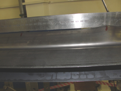
(a) Test 1: Close up of local buckling waves

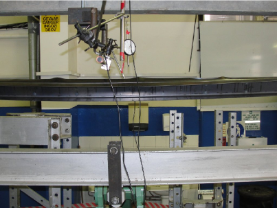
(b) Test 3

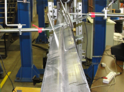
(c) Test 6

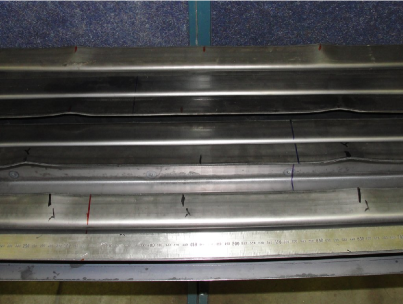
(d) Post-testing beams: Tests 1, 3, 4 and 5

Figure 13: Selection of photographs from the experimental programme: (a)–(c) all showing interactive buckling and (d) shows four of the beams and their locally buckled flanges that show plastic deformation.

which show the beams from a variety of directions while they were undergoing interactive buckling. In tests 2 and 6, there was visual experimental evidence of cellular buckling; Figure 14

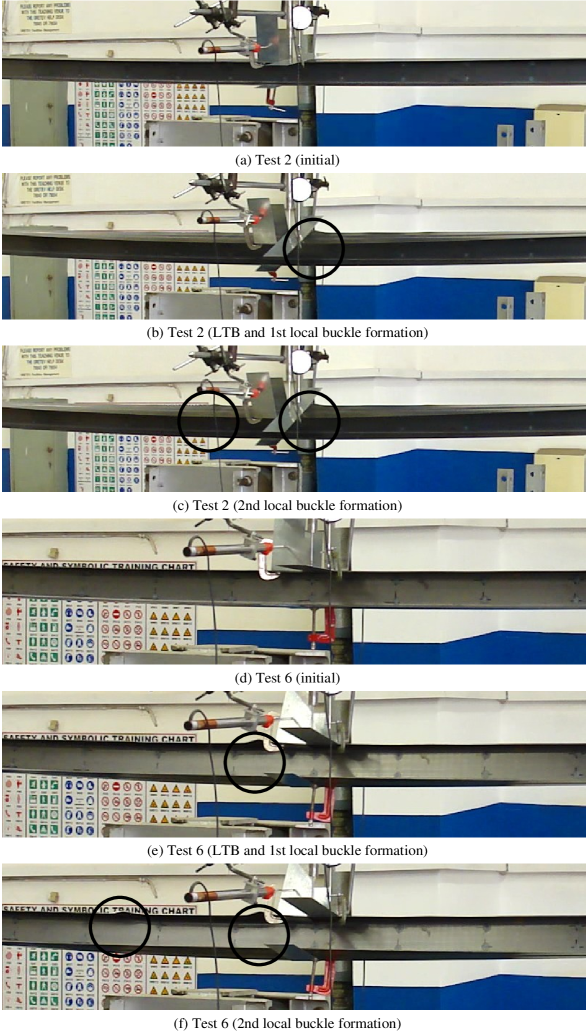
Figure 14: Evidence of cellular buckling. Two sequences of three photographs are shown of tests 2 (a)–(c) and 6 (d)–(f) respectively. Photographs (a) and (d) respectively show the pre-buckling state; (b) and (e) respectively show the initial post-buckling with one significant peak at midspan; (d) and (f) respectively show a newly developed local buckling peak in the top flange.

shows a sequence of photographs before and after the principal instability showing a new local buckling peak appearing soon after the initial one. Table 5

		Initial post-buckling	Local buckling mode observations
Test	$M_{\mathrm{max}}/M^{\mathrm{C}}$	drop in moment (%)	No. of visible	Extent
			buckling peaks	(% of $L_{e}$)
$1$	1.03	15	5	25.4
$2$	0.90	7	7	36.5
$3$	0.93	12	7	40.6
$4$	1.07	24	8	52.4
$5$	1.00	14	9	65.8
$6$	1.05	15	9	69.2

Table 5: Results from the experimental programme in terms of the maximum moment and the local buckling profile. The final column is a measure of localized nature of the flange buckle – the smaller the number, the more it was localized.

presents the results and their comparison with the individual buckling modes. The maximum applied moment in the experiments $M_{\mathrm{max}}$ is presented as a ratio of the theoretical critical moment $M^{\mathrm{C}}$ calculated from the appropriate critical mode given in Table 2, whether LTB or local buckling. The local buckling profile was determined by marking (as seen in Figure 13(d)) and measuring between adjacent peaks of the local buckling displacement over the length of the vulnerable part of the compression flange while the beam was still loaded but well after the peak moment had been applied. The interactive mode was clearly modulated in each case, with the peak amplitudes from local buckling decaying towards the lateral restraints; this was particularly notable in the cases where LTB was critical since the number of peaks was visibly fewer. In each test, two or three peaks of the local buckling mode exhibited significant plastic deformation almost immediately after the interactive mode was triggered; it was adjacent to these peaks where the buckling wavelength was, in general, measured to be the smallest values.

Another notable feature shown in Table 5 is the immediate proportional drop in the moment once the interactive mode had been triggered. As would be expected from the literature [31], the largest drop occurred in test 4 where the critical modes had been practically simultaneous. It is also noteworthy that the tests with identical buckling lengths (tests 1 and 2) showed very different peak moments and moment drops. A rational hypothesis can be devised for this by postulating that the beam in test 2 contained more geometric imperfections than the beam in test 1. This would not only account for the smaller maximum moment measured in test 2, but also for its smaller relative moment drop and its lower residual moment in the post-buckling range [9].

4.3.1 Comparisons with variational model and discussion

Figure 15

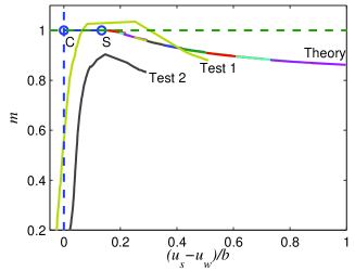
(a) Tests 1 and 2: $L_{e}=3200~{}\mbox{$\mathrm{mm}$}$

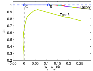
(b) Test 3: $L_{e}=3000~{}\mbox{$\mathrm{mm}$}$

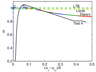
(c) Test 4: $L_{e}=2750~{}\mbox{$\mathrm{mm}$}$

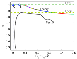
(d) Test 5: $L_{e}=2500~{}\mbox{$\mathrm{mm}$}$

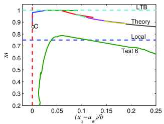
(e) Test 6: $L_{e}=2250~{}\mbox{$\mathrm{mm}$}$

Figure 15: Moment ratio $m$ versus bottom flange lateral displacement $(u_{s}-u_{w})/b$ for all the experiments with the variational model predictions superimposed, denoted as “Theory” and evaluated by Auto. Points $\mathrm{C}$ and $\mathrm{S}$ refer to the critical and secondary instability points obtained from the model. Note that local buckling was the theoretical critical instability mode for Tests 4–6.

presents normalized plots of the applied moment $m$ versus the measured and normalized lateral displacement of the bottom flange, $(u_{s}-u_{w})/b$. Test 4 gives clearly the best comparison in terms of the correlation between the post-buckling response of the actual beam and the model prediction. Tests 1 and 2 also show good basic agreement with the theory; test 1 showing that the post-buckling unloading resembles the theory quite well, while test 2 shows that the instability is triggered at a similar value of the lateral displacement predicted by the theory (see Table 6).

Test	$(u_{s}-u_{w})/b$		Local buckling wavelengths $\Lambda$ ($\mathrm{mm}$)
	Expt	Theory	Expt range	Expt average	Theory (minimum)
$1$	0.169	0.134	185 $\rightarrow$ 221	203	200
$2$	0.146	0.134	171 $\rightarrow$ 250	195	200
$3$	0.061	0.110	161 $\rightarrow$ 242	203	150
$4$	0.068	0.083	161 $\rightarrow$ 249	206	153
$5$	0.066	0.052	167 $\rightarrow$ 247	206	163
$6$	0.061	0.058	158 $\rightarrow$ 225	195	240

Table 6: Comparisons of the experimental results with the variational model in terms of the values of the bottom flange displacement at the peak moment point and the local buckling wavelengths.

Tests 5 and 6 clearly peak at or marginally above the local buckling critical moment, as predicted from linear analysis. However, in a similar way to test 2, the instability is triggered at a lateral displacement that correlates well with the prediction from the variational model. For test 6, the variational model yields a lower critical moment than the $M_{\mathrm{cr}}$ value for LTB, which triggers a quasi-local buckling mode. However, as stated earlier, a distinct and accurate local buckling mode can only be modelled with additional displacement functions in the current framework so this particular result needs to be interpreted with some caution. Test 3 could be considered to be an outlier, but the measured response would imply, in a similar way that was discussed above regarding test 2, that the level of geometric imperfections in this beam was higher than the other tested beams (1, 4, 5, 6). Hence, the measured instability moment is less, the unloading proportion is less and the response is practically parallel to the model curve, which in fact is encouraging.

In terms of the local buckling wavelengths, these are compared to the wavelength of the buckling profile obtained from the variational model as described in §4.2. Even though the theoretical results seemed to be influenced by effects close to the boundary (particularly in test 6), hence the variability in the predictions, the general correlation between the experiments and theory is good. The apparent confirmation that the post-buckling behaviour of an I-beam under pure bending is cellular when global and local instability modes interact nonlinearly poses the following question: is this phenomenon prevalent in other thin-walled structural components that are known to suffer from overall and local mode interaction? Compressed stringer-stiffened plates [7] and I-section struts [5] are prime examples of other components where local and global mode interactions are known to occur. Further research is obviously required to determine the answer.

5 Concluding remarks

The current work identifies an interactive form of buckling for an I-beam under uniform bending which couples a global instability with local buckling in one-half of the compression flange. In contrast to earlier, more numerical, work [13, 24], cellular buckling, the transformation from a localized to an effectively periodic mode, is predicted theoretically for the purely elastic case and evidenced in physical tests. The model compares well both qualitatively and quantitatively with the observed collapse of a beam that undergoes the interaction under discussion that involves global, local, localized and cellular buckling. The localized buckle pattern first appears at a secondary bifurcation point which immediately destabilizes a portion of the compression flange; as the deformation grows, the buckle tends to spread in cells until eventually it restabilizes when the localized buckling pattern has become periodic after a sequence of snap-backs.

Experimentally, the process is unstable and so this sequence occurs rapidly even under rigid loading with the local buckling cells being triggered dynamically. This highlights the practical dangers of the modelled and observed phenomenon; the interaction reduces the load carrying capacity, it therefore introduces an imperfection sensitivity that would need to be quantified such that robust design rules can be developed to mitigate against such hazardous structural behaviour.

Acknowledgements

The majority of this work was conducted while MAW was on sabbatical from April–October 2010 at the School of Civil and Environmental Engineering, University of the Witwatersrand, Johannesburg, South Africa. The authors are extremely grateful to the Head of School, Professor Mitchell Gohnert, the Senior Laboratory Technician, Kenneth Harman, and Spencer Erling from the South African Institute of Steel Construction for facilitating the experimental programme.

References

- [1] Hancock, G. J. Local, distortional and lateral buckling of I-beams. ASCE J. Struct. Div., 104(11):1787–1798, 1978.
- [2] Schafer, B. W. Local, distortional, and Euler buckling of thin-walled columns. ASCE J. Struct. Eng., 128(3):289–299, 2002.
- [3] Rasmussen, K. J. R. and Wilkinson, T., editors. Coupled instabilities in metal structures CIMS2008, volume 2: Gregory J. Hancock Symposium, Sydney, 2008. University Publishing Services, University of Sydney.
- [4] Timoshenko, S. P. and Gere, J. M. Theory of elastic stability. McGraw-Hill, New York, USA, 1961.
- [5] Becque, J. and Rasmussen, K. J. R. Experimental investigation of the interaction of local and overall buckling of stainless steel I-columns. J. Struct. Eng. – ASCE, 135(11):1340–1348, 2009.
- [6] Hunt, G. W. and Wadee, M. A. Localization and mode interaction in sandwich structures. Proc. R. Soc. A, 454(1972):1197–1216, 1998.
- [7] Koiter, W. T. and Pignataro, M. A general theory for the interaction between local and overall buckling of stiffened panels. Technical Report WTHD 83, Delft University of Technology, Delft, The Netherlands, 1976.
- [8] Pignataro, M., Pasca, M., and Franchin, P. Post-buckling analysis of corrugated panels in the presence of multiple interacting modes. Thin-Walled Struct., 36(1):47–66, 2000.
- [9] Thompson, J. M. T. and Hunt, G. W. A general theory of elastic stability. Wiley, London, 1973.
- [10] Cherry, S. The stability of beams with buckled compression flanges. The Structural Engineer, 38(9):277–285, Sept 1960.
- [11] Menken, C. M., Groot, W. J., and Stallenberg, G. A. J. Interactive buckling of beams in bending. Thin-Walled Struct., 12(5):415–434, 1991.
- [12] Goltermann, P. and Møllmann, H. Interactive buckling in thin walled beams—II. applications. Int. J. Solids Struct., 25(7):729–749, 1989.
- [13] Møllmann, H. and Goltermann, P. Interactive buckling in thin walled beams—I. theory. Int. J. Solids Struct., 25(7):715–728, 1989.
- [14] Doedel, E. J. and Oldeman, B. E. Auto-07p: Continuation and bifurcation software for ordinary differential equations. Technical report, Department of Computer Science, Concordia University, Montreal, Canada, 2009. Available from http://indy.cs.concordia.ca/auto/.
- [15] Hunt, G. W., Peletier, M. A., Champneys, A. R., Woods, P. D., Wadee, M. A., Budd, C. J., and Lord, G. J. Cellular buckling in long structures. Nonlinear Dyn., 21(1):3–29, 2000.
- [16] Burke, J. and Knobloch, E. Homoclinic snaking: Structure and stability. Chaos, 17(3):037102, 2007.
- [17] Hunt, G. W., Lord, G. J., and Champneys, A. R. Homoclinic and heteroclinic orbits underlying the post-buckling of axially-compressed cylindrical shells. Comput. Meth. Appl. Mech. Eng., 170:239–251, 1999.
- [18] Hunt, G. W., Lord, G. J., and Peletier, M. A. Cylindrical shell buckling: A characterization of localization and periodicity. Discrete Contin. Dyn. Syst.–Ser. B, 3(4):505–518, 2003.
- [19] Hunt, G. W., Peletier, M. A., and Wadee, M. A. The Maxwell stability criterion in pseudo-energy models of kink banding. J. Struct. Geol., 22(5):669–681, 2000.
- [20] Wadee, M. A. and Edmunds, R. Kink band propagation in layered structures. J. Mech. Phys. Solids, 53(9):2017–2035, 2005.
- [21] Pi, Y. L., Trahair, N. S., and Rajasekaran, S. Energy equation for beam lateral buckling. J. Struct. Eng. – ASCE, 118(6):1462–1479, 1992.
- [22] Hunt, G. W., Da Silva, L. S., and Manzocchi, G. M. E. Interactive buckling in sandwich structures. Proc. R. Soc. A, 417(1852):155–177, 1988.
- [23] Wang, C. M., Reddy, J. N., and Lee, K. H. Shear deformable beams and plates: Relationships with classical solutions. Elsevier, Amsterdam, 2000.
- [24] Menken, C. M., Schreppers, G. M. A., Groot, W. J., and Petterson, R. Analyzing buckling mode interactions in elastic structures using an asymptotic approach; theory and experiments. Comput. Struct., 64(1–4):473–480, 1997.
- [25] Wadee, M. A. Effects of periodic and localized imperfections on struts on nonlinear foundations and compression sandwich panels. Int. J. Solids Struct., 37(8):1191–1209, 2000.
- [26] Wadee, M. K. and Bassom, A. P. Characterization of limiting homoclinic behaviour in a one-dimensional elastic buckling model. J. Mech. Phys. Solids, 48(11):2297–2313, 2000.
- [27] Peletier, M. A. Sequential buckling: A variational analysis. SIAM J. Appl. Math., 32(5):1142–1168, 2001.
- [28] Budd, C. J., Hunt, G. W., and Kuske, R. Asymptotics of cellular buckling close to the Maxwell load. Proc. R. Soc. A, 457(2016):2935–2964, 2001.
- [29] Wadee, M. K., Coman, C. D., and Bassom, A. P. Solitary wave interaction phenomena in a strut buckling model incorporating restabilisation. Physica D, 163:26–48, 2002.
- [30] von Kármán, T., Sechler, E. E., and Donnell, L. H. The strength of thin plates in compression. Trans. ASME, 54(APM):54–55, 1932.
- [31] Budiansky, B., editor. Buckling of structures. IUTAM Symposium, Cambridge, USA, 1974. Springer, Berlin, 1976.