Large Scales – Long Times: Adding High Energy Resolution to SANS

Abstract

The Neutron Spin Echo (NSE) variant MIEZE (Modulation of IntEnsity by Zero Effort), where all beam manipulations are performed before the sample position, offers the possibility to perform low background SANS measurements in strong magnetic fields and depolarising samples. However, MIEZE is sensitive to differences $\Delta L$ in the length of neutron flight paths through the instrument and the sample. In this article, we discuss the major influence of $\Delta L$ on contrast reduction of MIEZE measurements and its minimisation. Finally we present a design case for enhancing a small-angle neutron scattering (SANS) instrument at the planned European Spallation Source (ESS) in Lund, Sweden, using a combination of MIEZE and other TOF options, such as TISANE offering time windows from ns to minutes. The proposed instrument would allow obtaining an excellent energy- and $Q$-resolution straightforward to µs for 0.01 Å^-1, even in magnetic fields, depolarising samples as they occur in soft matter and magnetism while keeping the instrumental effort and costs low.

1 Introduction

The Neutron Spin Echo technique (NSE) [1] in its different variants is a unique method for measuring dynamic processes in soft matter [2] and spin excitations in magnetic systems [3]. As it allows for the decoupling of the incoming wavelength distribution and the energy resolution, typically values in the neV to µeV regime can be reached. Contrary to backscattering NSE provides an excellent $Q$-resolution. There exist different methods for neutron spin echo measurements, namely classical neutron spin echo (NSE) [1] and neutron resonance spin echo (NRSE) [4]. The application of NSE and NRSE is currently limited to measurements with dedicated instruments, where neither the samples nor the sample environment may depolarise the beam.

A method similar to NRSE is the MIEZE (Modulation of IntEnsity by Zero Effort) [5] technique. As in MIEZE all spin manipulations are performed before the sample position it avoids the complications operating with polarised neutrons in strong magnetic fields or in a depolarising environment, like hydrogen containing samples, which introduce spin-flips. It can easily operate in any neutron scattering experiment with enough space before the sample and a detector with nanosecond time resolution. This method invented by Gähler and Golub [5] has also been demonstrated experimentally in the nineties for soft matter samples [6, 7, 8, 9]. Recently we published MIEZE measurements on the itinerant magnet MnSi in a magnetic field [10] demonstrating the power of the method for magnetic applications.

MIEZE is easily implemented as an option at many instruments, provided a fast detector exists. It can add energy resolution down to the sub-µeV region, mainly in the small angle regime. This paper aims to develop the tools necessary for designing a MIEZE option for a SANS instrument adding high energy resolution to it.

2 Modulation of IntEnsity by Zero Effort (MIEZE)

MIEZE uses the first arm of an NRSE instrument, followed by a polarisation analyser in front of the sample and a fast neutron detector with ns time-resolution (see figure 1b). In the following we use the wave packet description of the coarse monochromatised neutron beam. For a detailed quantum mechanical description see [11]. While in NRSE, all coils are operated at the same frequency [12] , in MIEZE, the two coils are driven at different frequencies, $\nu_{1}=\omega_{1}/2\pi$ and $\nu_{2}=\omega_{2}/2\pi$, with $\nu_{2}>\nu_{1}$. This leads to an overcompensation of the energy splitting of the spin up $\left|\uparrow\right\rangle$ and spin down $\left|\downarrow\right\rangle$ wave packets in the second coil as shown in figure 1c. As $\left|\uparrow\right\rangle$ and $\left|\downarrow\right\rangle$ are now propagating with different velocities, they are interfering only at the specific distance

$$L_{2}=\frac{L_{1}}{\omega_{2}/\omega_{1}-1}$$ (1)

after the last coil. At this position, one obtains a time beating signal depending on the difference of the two coil frequencies (see figure 1a) of the form

$$I(t)={\textstyle\frac{1}{2}}I_{0}(1+C\cdot\cos{\omega_{M}t}),$$ (2)

where $\omega_{M}=2\cdot(\omega_{2}-\omega_{1})$ is the frequency difference of the two NRSE coils. $C=\frac{I_{+}-I_{-}}{I_{+}+I_{-}}$ is the contrast, which is given by the ratio of the measured amplitude $A$ and the average intensity $B$ (figure 1a).

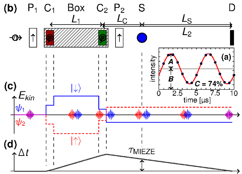
Figure 1: (a)  A typical MIEZE signal at the detector position (see text for details). (b) Schematic of a complete MIEZE setup, showing the polariser (P₁), the zero field of the MIEZE box (hatched) with two $\pi$-flipper coils (C₁, C₂), the analyser (P₂), the sample (S) and the detector (D). (c) Kinetic energy splitting for the spin-down ($\psi_{1}$) and spin-up ($\psi_{2}$) states of the neutrons along the flight path due to the $\pi$-flipper coils. (d) Temporal delay $\Delta t$ of the spin states along the flight path. The splitting reaches its maximum after the second flipper coil and vanishes at the detector position (after [10]).
Reprinted with permission from APS. ©2011, American Institute of Physics.

The MIEZE time, which is equivalent to the spin echo time [12] is given by

$$\tau_{M}=\frac{\hbar}{mv^{3}}\omega_{M}L_{S},$$ (3)

where $L_{S}$ is the distance between sample and detector. Similar to time-of-flight methods, the time resolution obtained depends on $L_{S}$ as seen in figure 1d.

The role of the polarisation in NSE and NRSE is now taken by the contrast $C$ of the time beating signal, which can be expressed as

$$C=\int\!\text{d}\omega\,S(\omega)\cos(\omega\tau_{M}).$$ (4)

In analogy to NSE, a signal measured at a specific spin-echo time $\tau_{M}$ is directly proportional to the intermediate scattering function $S(Q,\tau_{M})$. Thus a typical MIEZE experiment results in the determination of $S(Q,\tau_{M})/S_{el}(Q,\tau_{M})$ over $\tau_{M}$, where $S_{el}(Q,\tau_{M})$ is the signal of an elastic reference sample, usually graphite or the sample in a frozen state (like very low T in the case of magnetic systems). For quasi-elastic experiments with an assumed Lorentzian line shape of half-width $\Gamma$, the normalised intermediate scattering function is given by [12]

$$\frac{S(Q,\tau_{M})}{S_{el}(Q,\tau_{M})}=\exp\left(-\Gamma(Q)\tau_{M}\right).$$ (5)

3 Path lengths in MIEZE

The MIEZE method is closely related to TOF methods and therefore sensitive to path length differences $\Delta L$. $\Delta L$ increases for larger $Q$. Therefore, the two different spin states interfere less with each other leading to a reduction in the contrast $C$. The path length differences originate from different parts of the MIEZE setup and can be expressed by

$$C=R_{\text{Coils}}\cdot R_{\text{Sample}}(\text{geometry},\Theta,\Lambda)\cdot R_{\text{Detector}}(\Lambda)\cdot C_{0},$$ (6)

where $\Theta$ is the scattering angle, $\Lambda=2\pi v/\omega_{M}$ the ratio of neutron velocity and angular frequency of the time-beating signal, i.e. the path length of one oscillation, and “geometry” denotes the sample geometry. $R_{\text{Coils}}$ contains the contrast reduction in the coil systems in front of the beam. $R_{\text{Coils}}$ is mainly determined by the performance of the flipper coils and the perfection of the zero field shielding around the system. $R_{\text{Detector}}$ treats the loss of contrast due to the thickness of the detector. Depending on the interaction depth of the neutrons in the detector, the flight paths of the neutrons are different, thus reducing the contrast of the intensity modulation. As an example, the instrument MIRA [13] at the FRM II will use a CASCADE detector [14, 15] with 2 µm thick neutron detection planes. Therefore, $R_{\text{Detector}}$ is approximately 1.

The reduction factors $R_{\text{Coils}}$ and $R_{\text{Detector}}$ depend only on instrument specific parameters, therefore they can be determined by experiment or theoretical calculations independently of a specific sample.

In contrast, $R_{\text{Sample}}$ depends both on the geometry of the experiment and the sample and needs to be treated separately for each experiment. While Hayashida et al. [16] determined this reduction factor through Monte-Carlo simulations, we present here analytical formulae, which can be calculated faster and provide more insight into the influence of different sample geometries on $C$. For simplicity we neglect here the influence of the divergence in the beam, as it anyhow is for SANS quite small.

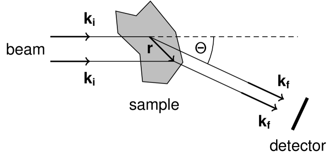
Figure 2: The scattering geometry: A parallel beam of neutrons is scattered by the whole sample volume under the angle $\Theta$.

Figure 3: Definition of the dimensions of different sample shapes.

The path length difference $\Delta L$ caused by scattering of a parallel incoming beam in a sample at two different positions of interaction separated by $\mathbf{r}$ (see figure 2) is given in first order by [17]

$$\Delta L(\mathbf{r})=\left(\frac{\mathbf{k_{i}}}{|\mathbf{k_{i}}|}-\frac{\mathbf{k_{f}}}{|\mathbf{k_{f}}|}\right)\cdot\mathbf{r}.$$ (7)

This corresponds to a phase shift of $\Delta\phi(\mathbf{r})=\omega_{M}\Delta L(\mathbf{r})/v=2\pi\Delta L(\mathbf{r})/\Lambda$, where $\Lambda$, as defined above, is the path length for a single oscillation. Integrating over the total sample volume $V$ yields

$$C = \int\text{d}\omega\,S(\omega)\frac{1}{V}\int_{\text{Sample}}\kern-19.91692pt\text{d}^{3}r\,\cos(\omega\tau_{M}+\Delta\phi(\mathbf{r}))$$ (8)

$$= \int\text{d}\omega\,S(\omega)\frac{1}{V}\int_{\text{Sample}}\kern-19.91692pt\text{d}^{3}r\,\big{(}\cos(\omega\tau_{M})\cos\Delta\phi(\mathbf{r})-$$

$$\qquad\qquad\qquad\qquad\sin(\omega\tau_{M})\sin\Delta\phi(\mathbf{r})\big{)}\,.$$

For the Lorentzian $S(\omega)$ assumed earlier, the sin-term vanishes when integrating over $\omega$ and the integration separates into

$$C=\underbrace{\frac{1}{V}\int_{\text{Sample}}\kern-19.91692pt\text{d}^{3}r\,\cos\Delta\phi(\mathbf{r})}_{R_{\text{Sample}}}\underbrace{\int_{\vphantom{\text{Sample}}}\text{d}\omega\,S(\omega)\cos(\omega\tau_{M})}_{C_{0}}.$$ (9)

From this equation and the geometry given in figure 2 we can derive the correction factor for different sample shapes, with the dimensions given in figure 3:

1. Sphere with radius $r$:

   $$R(r,\Theta,\Lambda)=\frac{3\Lambda^{3}}{64\pi^{3}r^{3}}\frac{\sin\left(\frac{4\pi r}{\Lambda}\sin\frac{\Theta}{2}\right)}{\sin^{3}\frac{\Theta}{2}}-\frac{3\Lambda^{2}\cos\left(\frac{4\pi r}{\Lambda}\sin\frac{\Theta}{2}\right)}{16\pi^{2}r^{2}}.$$

2. Cylinder with radius $r$:

   $$R(r,\Theta,\Lambda)=\frac{\Lambda}{2\pi r}\frac{J_{1}\left(\frac{4\pi r}{\Lambda}\sin\frac{\Theta}{2}\right)}{\sin\frac{\Theta}{2}},$$

   where $J_{1}$ is the Bessel function of the first kind. The height $h$ of the cylinder – as it is oriented perpendicular to the scattering plane – does not affect the reduction factor $R$ for a parallel incoming beam.

3. Cuboid with thickness $d$ and width $a$:

   $$R(d,a,\Theta,\Lambda)=\frac{\Lambda^{2}}{4\pi^{2}da}\frac{\sin\left(\frac{2\pi a}{\Lambda}\cos\frac{\Theta}{2}\sin\frac{\Theta}{2}\right)\sin\left(\frac{2\pi d}{\Lambda}\sin^{2}\frac{\Theta}{2}\right)}{\sin^{3}\frac{\Theta}{2}\cos\frac{\Theta}{2}}.$$

   As for the cylinder the reduction factor R does not depend on $h$.

4. Disk with thickness $d$ and radius $r$:

   $$R(d,r,\Theta,\Lambda) = \frac{\Lambda^{2}}{4\pi^{3}dr^{2}}\frac{\sin\left(\frac{2\pi d}{\Lambda}\sin^{2}\frac{\Theta}{2}\right)}{\sin^{3}\frac{\Theta}{2}\cos\frac{\Theta}{2}}\cdot$$

   $$\int_{-r}^{r}\!\!\text{d}z\,\sin\left(\frac{2\pi\sqrt{r^{2}-z^{2}}}{\Lambda}\sin\Theta\right).$$

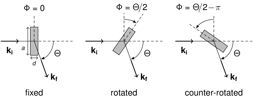
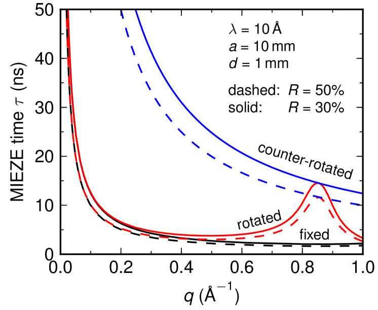
Figure 4: The $Q$, $\tau_{M}$ parameter space for a MIEZE instrument with $\lambda=10$Å, and a cuboid sample with $a=10$ mm and $d=1$ mm. The lines indicate where the contrast for different sample configurations is reduced to 50% and 30%. The sample is either not rotated at all, or rotated by half the scattering angle with respect to two different positions at $\Theta=0$.

By rotation of any plate-like sample (cuboid or disk) by $\Phi=\Theta/2-\pi$ (called “counter-rotation”, see figure 4), one obtains:

$$R(d,\Theta,\Lambda) = \frac{\Lambda}{2\pi d}\frac{\sin\left(\frac{2\pi d}{\Lambda}\sin\frac{\Theta}{2}\right)}{\sin\frac{\Theta}{2}}.$$

This results in a much slower decrease of $R$ with increasing $\Theta$ as $R$ depends only on $d$, the thickness of the sample, which can be made small.

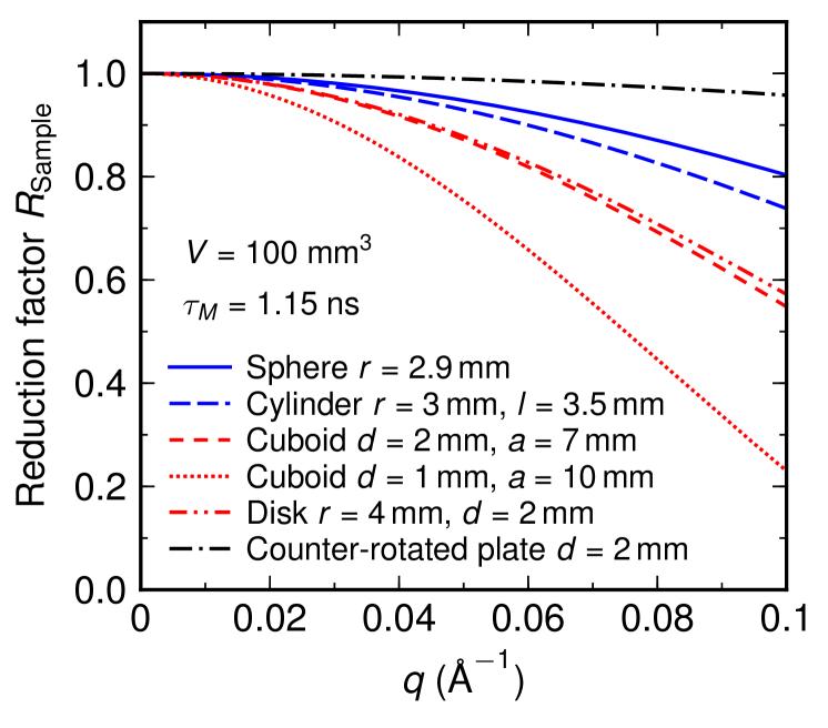
Figure 5: The reduction factor $R_{\text{Sample}}$ for different geometries with the same sample volume of $100\,\text{mm}^{3}$. It is calculated for the instrument parameters of MIRA with a wavelength $\lambda$ of 10.4 Å. $L_{1}$ is 1 m, and $L_{S}$ is 0.8 m. $\omega_{M}$ is $2\pi\cdot 200$ kHz, corresponding to $\tau_{M}=1.15$ ns. The scattering geometry is defined as shown in figure 2.

In figure 5 the reduction factor $R_{\text{Sample}}$ is plotted versus $Q=\frac{4\pi}{\lambda}\sin{\frac{\Theta}{2}}$ for different geometries of the sample. It becomes obvious that differences are only important for larger $Q$ values, and that there are large differences between different sample shapes.

In figure 4 the effect of sample rotation for measurements on cuboidal samples is demonstrated. The accessible parameter space in $Q$ and $\tau_{M}$ can be enlarged when turning the sample by half the scattering angle, in the right direction.

These theoretical predictions were tested for a cuboid of thickness $d=5$ mm and width $a=25$ mm using the MIEZE setup at FRM II [10] and a very good agreement for various $\tau_{M}$ is obtained as shown in figure 6.

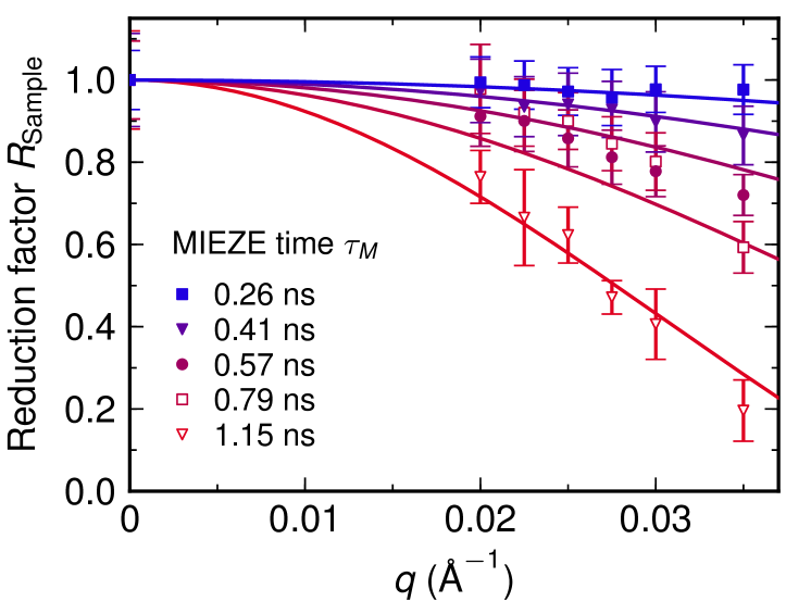
Figure 6: The reduction factor $R$ versus $Q$ for a cuboid of width $a=25$ mm and thickness $d=5$ mm compared to measured values of $R$ on the instrument MIRA with a wavelength $\lambda$ of 10.4 Å. $L_{1}$ is 1 m, and $L_{S}$ is 0.8 m. $\omega_{M}$ ranges from $2\pi\cdot 46$ kHz to $2\pi\cdot 200$ kHz, yielding a MIEZE time $\tau_{M}$ from 0.26 ns to 1.15 ns, respectively.

4 High resolution MISANS at ESS

From the discussion above it becomes clear that the MIEZE technique is particularly well suited for measurements in the small angle regime as for low $Q$ the contrast reduction due to the path length differences is less severe. Therefore a combination of a time-of-flight SANS instrument with a MIEZE option (MISANS) would allow for high resolution measurements both in energy- and Q-space. The MIEZE principle at a time-of-flight source was recently demonstrated at the chopped CG-1D beam at HFIR at the Oak Ridge National Laboratory [18].

Equations (1) and (3) demonstrate that the different instrument design parameters are correlated. If $L_{2}$ is replaced by $L_{2}=L_{C}+L_{S}$, where $L_{C}$ is the distance between the last coil and the sample (see figure 1b), one obtains

$$\tau_{M}=\frac{2\hbar\omega_{1}L_{S}L_{1}}{mv^{3}(L_{S}+L_{C})}\,.$$ (10)

This equation now allows for trading off different instrument designs if one defines the maximum range of Spin-Echo times.

Current NSE measurements are performed up to 1 µs [19] and are a benchmark for new spin echo beam lines. Considering typical SANS setups as proposed for long-pulse spallation sources such as the ESS [20] a zero-field region can be added to the 20 m long collimation section, with a coil distance, for example, $L_{1}=15$ m, a coil-sample distance $L_{C}=5$ m and a sample-detector distance $L_{S}=10$ m. For neutrons with $\lambda=20$ Å, which is a typical wavelength used in NSE for high resolution measurements, the remaining free parameter in eq. (10) is $\omega_{1}$. To achieve $\tau_{M}=1$ µs with this setup, the coils have to be driven at $\omega_{1}=2\pi\cdot 1$ MHz and $\omega_{2}=2\pi\cdot 2$ MHz so that $\omega_{M}=2\pi\cdot 2$ MHz. This can be obtained with current coil designs: RF coils that can be driven at these frequencies are in commissioning at the instruments RESEDA [21] and TRISP [22] at FRM II.

For these instrument parameters, a $\tau_{M}$–$Q$ parameter space is opened as shown in figure 7 for cuboid samples of several sizes. MIEZE times of 1 µs are achieved up to $Q=5\times 10^{-3}$ Å^-1 for samples with a width of 5 mm and a thickness of 2 mm. The largest spin echo times are available for small $Q$, which matches the requirements of measuring quasi-elastic dynamics, i.e. very slow relaxation processes as they are expected for large scale structures, for example in soft matter and magnetic materials with novel topological structures.

We do not discuss the $Q$ resolution of such an instrument here, as it is mainly defined by $\Delta\lambda/\lambda$, which is already small at a pulsed source, $\approx 3\%$ at the ESS as discussed in [20], and by the beam divergence, which will also be excellent for such a long collimation section.

In conclusion, we propose to rather dramatically enhance the capabilities of a SANS beam line at the ESS with different options to obtain in parallel information on structure and dynamics, especially in magnetic fields. These options can be MIEZE, TISANE [23] and stroboscopic SANS [24]. The latter two are basically available free of charge with the fast time-resolving detector for MIEZE. They will cover the time domain from nanoseconds to minutes. Such an instrument based on existing technology would open new perspectives for research in magnetic systems and soft matter. It would offer an excellent $q$-resolution and at the same time allow to measure the dynamics on a wide range of time scales, competitive to NSE or NRSE instruments. It would also be much cheaper and easier to build due to the reduced effort in magnetic shielding. Furthermore it allows to use modern focusing neutron optics in any part of the instrument, enhancing the intensity at the sample.

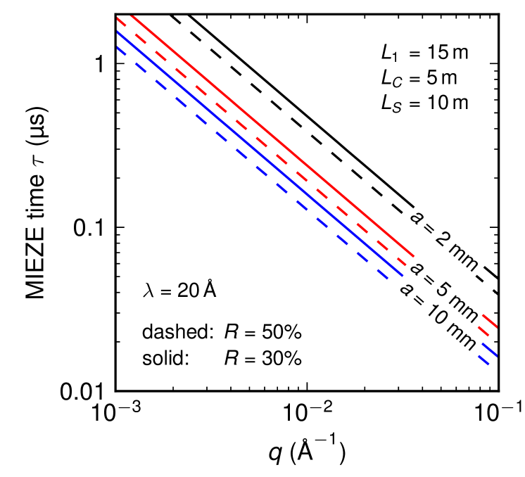
Figure 7: The $Q$, $\tau_{M}$ parameter space for a MISANS instrument at the ESS, assuming a fixed cuboid sample of several different widths $a$ and a thickness of $b=2$ mm. It is shown where the contrast for the different samples is reduced to 50% (the dashed lines), or to 30% (the solid lines).

5 Acknowledgment

We acknowledge very helpful discussions with J. Neuhaus, T. Keller, K. Habicht, C. Pfleiderer, M. Bleuel and J. Lal. This work is supported by the BMBF under “Mitwirkung der Zentren der Helmholtz Gemeinschaft und der Technischen Universität München an der Design-Update Phase der ESS, Förderkennzeichen 05E10WO1.”

References

- Mezei [1972] F. Mezei, Neutron spin echo: A new concept in polarized thermal neutron techniques, Zeitschrift für Physik A 255 (2) (1972) 146–160, doi:10.1007/BF01394523.
- Richter et al. [2005] D. Richter, M. Monkenbusch, A. Arbe, J. Colmenero, Neutron Spin Echo in Polymer Systems, Advances in Polymer Science 174 (2005) 1–221, doi:10.1007/b106578.
- Mezei [1984] F. Mezei, Critical Dynamics In Isotropic Ferromagnets, Journal of Magnetism and Magnetic Materials 45 (1) (1984) 67–73, doi:10.1016/0304-8853(84)90374-3.
- Golub and Gähler [1987] R. Golub, R. Gähler, A neutron resonance spin echo spectrometer for quasi-elastic and inelastic scattering, Physics Letters A 123 (1) (1987) 43–48, ISSN 0375-9601, doi:10.1016/0375-9601(87)90760-2.
- Gähler et al. [1992] R. Gähler, R. Golub, T. Keller, Neutron resonance spin echo–a new tool for high resolution spectroscopy, Physica B: Condensed Matter 180-181 (2) (1992) 899–902, doi:10.1016/0921-4526(92)90503-K.
- Köppe et al. [1996] M. Köppe, P. Hank, J. Wuttke, W. Petry, R. Gähler, R. Kahn, Performance and future of a neutron resonance spinecho spectrometer, Journal for Neutron Research 4 (1) (1996) 261–273, doi:10.1080/10238169608200092.
- Hank et al. [1997] P. Hank, W. Besenböck, R. Gähler, M. Köppe, Zero-field neutron spin echo techniques for incoherent scattering, Physica B: Condensed Matter 234-236 (1997) 1130–1132, doi:10.1016/S0921-4526(97)89269-1.
- Besenböck et al. [1998] W. Besenböck, R. Gähler, P. Hank, R. Kahn, M. Köppe, C.-H. de Novion, W. Petry, J. Wuttke, First scattering experiment on MIEZE: A fourier transform time-of-flight spectrometer using resonance coils, Journal for Neutron Research 7 (1) (1998) 65–74, doi:10.1080/10238169808200231.
- Köppe et al. [1999] M. Köppe, M. Bleuel, R. Gähler, R. Golub, P. Hank, T. Keller, S. Longeville, U. Rauch, J. Wuttke, Prospects of resonance spin echo, Physica B: Condensed Matter 266 (1-2) (1999) 75–86, doi:10.1016/S0921-4526(98)01496-3.
- Georgii et al. [2011] R. Georgii, G. Brandl, N. Arend, W. Häußler, A. Tischendorf, C. Pfleiderer, P. Böni, J. Lal, Turn-key module for neutron scattering with sub-micro-eV resolution, Applied Physics Letters 98 (7) (2011) 073505, doi:10.1063/1.3556558.
- Arend et al. [2004] N. Arend, R. Gähler, T. Keller, R. Georgii, T. Hils, P. Böni, Classical and quantum-mechanical picture of NRSE–measuring the longitudinal Stern-Gerlach effect by means of TOF methods, Physics Letters A 327 (1) (2004) 21–27, doi:10.1016/j.physleta.2004.04.062.
- Keller et al. [2002] T. Keller, R. Golub, R. Gähler, Neutron Spin Echo–A Technique for High-Resolution Neutron Scattering, in: R. Pike, P. Sabatier (Eds.), Scattering, Academic Press, London, ISBN 978-0-12-613760-6, 1264–1286, doi:10.1016/B978-012613760-6/50068-1, 2002.
- Georgii et al. [2007] R. Georgii, P. Böni, M. Janoschek, C. Schanzer, S. Valloppilly, MIRA–A flexible instrument for VCN, Physica B 397 (1-2) (2007) 150–152, doi:10.1016/j.physb.2007.02.088.
- Häußler et al. [2011] W. Häußler, P. Böni, M. Klein, C. J. Schmidt, U. Schmidt, F. Groitl, J. Kindervater, Detection of high frequency intensity oscillations at RESEDA using the CASCADE detector, Review of Scientific Instruments 82 (4) (2011) 045101, doi:10.1063/1.3571300.
- Klein and Schmidt [2011] M. Klein, C. J. Schmidt, CASCADE, neutron detectors for highest count rates in combination with ASIC/FPGA based readout electronics, in: Nuclear Instruments and Methods in Physics Research Section A: Accelerators, Spectrometers, Detectors and Associated Equipment, vol. 628, 9–18, doi:%****␣MIEZE_design.tex␣Line␣600␣****10.1016/j.nima.2010.06.278, 2011.
- Hayashida et al. [2008] H. Hayashida, M. Hino, M. Kitaguchi, Y. Kawabata, N. Achiwa, A study of resolution function on a MIEZE spectrometer, Measurement Science and Technology 19 (2008) 4006, doi:10.1088/0957-0233/19/3/034006.
- Keller [1993] T. Keller, Höchstauflösende Neutronenspektrometer auf Basis von Spinflippern – neue Varianten des Spinecho-Prinzips, Ph.D. thesis, Technische Universität München, 1993.
- Brandl et al. [2011] G. Brandl, R. Georgii, M. Bleuel, J. Carpenter, L. Robertson, L. Crow, J. Lal, Measurements on MnSi with MISANS, to be published in: Journal of Physics: Conference Series .
- Ohl et al. [2004] M. Ohl, M. Monkenbusch, D. Richter, C. Pappas, The high-resolution neutron spin-echo spectrometer for the SNS with s, Physica B: Condensed Matter 350 (2004) 147–150, doi:10.1016/j.physb.2004.04.014.
- Schober et al. [2008] H. Schober, E. Farhi, F. Mezei, P. Allenspach, K. Andersen, P. M. Bentley, P. Christiansen, B. Cubitt, R. K. Heenan, J. Kulda, P. Langan, K. Lefmann, K. Lieutenant, M. Monkenbusch, P. Willendrup, J. Saroun, P. Tindemans, G. Zsigmond, Tailored instrumentation for long-pulse neutron spallation sources, Nuclear Instruments and Methods in Physics Research Section A: Accelerators, Spectrometers, Detectors and Associated Equipment 589 (1) (2008) 34–46, doi:10.1016/j.nima.2008.01.102.
- Häußler et al. [2008] W. Häußler, D. Streibl, P. Böni, RESEDA: Double and Multi Detector Arms for Neutron Resonance Spin Echo Spectrometers, Measurement Science and Technology 19 (2008) 034015, doi:10.1088/0957-0233/19/3/034015.
- Keller et al. [2007] T. Keller, P. Aynajian, S. Bayrakci, K. Buchner, K. Habicht, H. Klann, M. Ohl, B. Keimer, The Triple Axis Spin-Echo Spectrometer TRISP at the FRM II, Neutron News 18 (2) (2007) 16–18, doi:10.1080/10448630701328372.
- Kipping et al. [2008] D. Kipping, R. Gähler, K. Habicht, Small angle neutron scattering at very high time resolution: Principle and simulations of ’TISANE’, Physics Letters A 372 (10) (2008) 1541–1546, doi:10.1016/j.physleta.2007.10.041.
- Keiderling and Wiedenmann [2007] U. Keiderling, A. Wiedenmann, Field-dependent relaxation behavior of Co-ferrofluid investigated with stroboscopic time-resolved small-angle neutron scattering, Journal of Applied Crystallography 40 (s1) (2007) s62–s67, doi:10.1107/S0021889806047650.