Numerical analysis of cosmological models for accelerating Universe in Poincaré gauge theory of gravity

Abstract

Homogeneous isotropic models with two torsion functions built in the framework of the Poincaré gauge theory of gravity based on general expression of gravitational Lagrangian by certain restrictions on indefinite parameters are analyzed numerically. Special points of cosmological solutions at asymptotics and conditions of their stability in dependence of indefinite parameters are found. Procedure of numerical integration of the system of gravitational equations at asymptotics is considered. Numerical solution for accelerating Universe without dark energy and dark matter is obtained. It is shown that by certain restrictions on indefinite parameters obtained cosmological solutions are in agreement with SNe Ia observational data and Big Bang Nucleosynthesis predictions. Statefinder diagnostics is discussed in order to compare considered cosmological model with other models.

1 Introduction

One of the most principal recent achievements of observational cosmology is the discovery of the acceleration of cosmological expansion at present epoch [1, 2]. In order to explain this observable accelerating cosmological expansion in the framework of General Relativity Theory (GR), the notion of dark energy (or quintessence) was introduced in cosmology. According to obtained estimations, approximately 70% of energy in our Universe is related with some hypothetical kind of gravitating matter with negative pressure — “dark energy” — of unknown nature. Previously a number of investigations devoted to dark energy problem (DEP) were carried out (see reviews [3, 4]).

According to widely known opinion, the dark energy is associated with cosmological term, which is related in the framework of standard $\Lambda CDM$-model to the vacuum energy density of quantized matter fields. In connection with this the following question appears: why the value of cosmological term is very small and close to average energy density in the Universe at present epoch (see for example [5]). Other treatment to solve the DEP is connected with modification of gravitation theory.

One of such solutions can be obtained in the framework of gravitation theory in the Riemann-Cartan spacetime $U_{4}$ - Poincaré gauge theory of gravity (PGTG) [6, 7, 8, 9, 10]. It should be noted that the PGTG is a natural and in certain sense necessary generalization of metric theory of gravitation by including the Lorentz group to the gauge group which corresponds to gravitational interaction. The PGTG leads to the change of gravitational interaction in comparison with GR and Newton’s theory of gravity at cosmological scale, which are provoked by more complicated structure of physical spacetime, namely by spacetime torsion [11, 12].

Explicit form of gravitational equations of PGTG and their physical consequences depend essentially on the structure of gravitational Lagrangian ${\cal L}_{\mathrm{g}}$, which is built by means of invariants of gravitational gauge field strengths — the curvature and torsion tensors. The most simple PGTG is Einstein-Cartan theory based on the gravitational Lagrangian in the form of scalar curvature of spacetime $U_{4}$ [13]. In the frame of Einstein-Cartan theory the DEP was discussed in [14], where some phenomenological description of spinning matter was used. In connection with this it should be noted that in the frame of Einstein-Cartan theory the torsion is connected with spin momentum by linear algebraic relation and vanishes in the case of spinless matter. Such situation seems unnatural by taking into account that the torsion tensor is gravitational gauge strength corresponding to transformations of translations, which are connected directly with energy-momentum tensor in the frame of Noether formalism. The situation comes to normal by including to ${\cal L}_{\mathrm{g}}$ terms quadratic in the curvature and torsion tensors.

The most general form of the gravitational Lagrangian ${\cal L}_{\mathrm{g}}$ (without using Levi-Civita symbol) includes the linear in the scalar curvature term as well as 9 quadratic terms (6 invariants of the curvature tensor and 3 invariants of the torsion tensor with indefinite parameters). The structure of the gravitational equations and physical consequences of isotropic cosmology in the frame of PGTG, in particular, the situation concerning the DEP depend essentially on restrictions on indefinite parameters. The PGTG can be divided into different sectors in dependence on the number of nonvanishing componets of the torsion tensor and the order of the differential equations determining their behaviour and behaviour of the scale factor that is connected with restrictions on indefinite parameters of ${\cal L}_{\mathrm{g}}$.

In general case the torsion tensor for homogeneous isotropic models (HIM) is described by two functions of time $S_{1}$ and $S_{2}$ determining trace and pseudotrace of the torsion tensor respectively. At the first time the most simple HIM with the only nonvanishing torsion function $S_{1}$ were built and investigated in [15]; it was shown that by certain restrictions on equation of state of gravitating matter at extreme conditions (extremely high energy densities and pressures) in the beginning of cosmological expansion all cosmological solutions are regular with respect to metrics, Hubble parameter, its time derivative and energy density by virtue of gravitational repulsion effect at extreme conditions (see [16]). The regular Big Bang scenario with inflationary stage in the beginning of cosmological expansion based on such HIM was built and analyzed in [17, 18].

Other sector of PGTG is so-called dynamical scalar torsion sector considered in [19, 20]. HIM biult in this sector demonstrate the oscillating behaviour of the Hubble parameter, and it is possible to obtain good correspondence with SNe Ia observational data.

By investigation the sector of PGTG with two torsion functions it was shown that the PGTG allows to explain the acceleration of cosmological expansion at present epoch without using the notion of dark energy [21]. This result is due to the fact, that the cosmological equations for HIM at asymptotics take the form of Friedmann cosmological equations of GR with effective cosmological constant induced by spacetime torsion if certain restrictions on indefinite parameters of gravitational Lagrangian are imposed. As it was shown in [25], isotropic cosmology based on HIM with two torsion functions offers opportunities to solve also the problem of dark matter. The analysis of regular inflationary cosmological models built on the base of HIM with two torsion functions by certain restrictions on indefinite parameters in gravitational equations for such models was fulfilled in [26]. The present paper is devoted to numerical analysis of HIM with two torsion functions of accelerating Universe at asymptotics when energy densities are sufficiently small.

2 Cosmological equations for homogeneous isotropic models

In this Section we briefly repeat the derivation of the cosmological equations for HIM with two torsion functions (see [21, 26]).

In the framework of PGTG the role of gravitational field variables play the tetrad $h^{i}{}_{\mu}$ and the Lorentz connection $A^{ik}{}_{\mu}$; corresponding field strengths are the torsion tensor $S^{i}{}_{\mu\nu}$ and the curvature tensor $F^{ik}{}_{\mu\nu}$ defined as

$$S^{i}{}_{\mu\,\nu}=\partial_{[\nu}\,h^{i}{}_{\mu]}-h_{k[\mu}A^{ik}{}_{\nu]}\,,$$

$$F^{ik}{}_{\mu\nu}=2\partial_{[\mu}A^{ik}{}_{\nu]}+2A^{il}{}_{[\mu}A^{k}{}_{|l\,|\nu]}\,,$$

where holonomic and anholonomic space-time coordinates are denoted by means of greek and latin indices respectively.

We will consider the PGTG based on gravitational Lagrangian given in the following general form

$${\cal L}_{\mathrm{g}}=f_{0}\,F+F^{\alpha\beta\mu\nu}\left(f_{1}\>F_{\alpha\beta\mu\nu}+f_{2}\>F_{\alpha\mu\beta\nu}+f_{3}\>F_{\mu\nu\alpha\beta}\right)+F^{\mu\nu}\left(f_{4}\>F_{\mu\nu}+f_{5}\>F_{\nu\mu}\right)$$

$$+f_{6}\>F^{2}+S^{\alpha\mu\nu}\left(a_{1}\>S_{\alpha\mu\nu}+a_{2}\>S_{\nu\mu\alpha}\right)+a_{3}\>S^{\alpha}{}_{\mu\alpha}S_{\beta}{}^{\mu\beta},$$ (2.1)

where $F_{\mu\nu}=F^{\alpha}{}_{\mu\alpha\nu}$, $F=F^{\mu}{}_{\mu}$, $f_{i}$ ($i=1,2,\ldots,6$), $a_{k}$ ($k=1,2,3$) are indefinite parameters, $f_{0}=(16\pi G)^{-1}$, $G$ is Newton’s gravitational constant (the velocity of light in the vacuum is equal to 1). Gravitational equations of PGTG obtained from the action integral $I=\int{\left({\cal L}_{\mathrm{g}}+{\cal L}_{\mathrm{m}}\right)\,}h\,d^{4}x$, where $h=\det{\left(h^{i}{}_{\mu}\right)}$ and ${\cal L}_{\mathrm{m}}$ is the Lagrangian of gravitating matter, contain the system of 16+24 equations corresponding to gravitational variables $h^{i}{}_{\mu}$ and $A^{ik}{}_{\mu}$. The sources of gravitational field in PGTG are the energy-momentum and spin tensors. In present paper we will consider perfect fluid with energy density $\rho$, pressure $p=p(\rho)$ and vanishing spin tensor as a source of gravitational field.

High spatial symmetry of HIM allows to describe these models by three functions of time $t$: the scale factor of Robertson-Walker metrics $R$ and two torsion functions $S_{1}$ and $S_{2}$ determining the curvature functions $A_{k}$ ($k=1,2,3,4$) as following

$$A_{1}=\dot{H}+H^{2}-2HS_{1}-2\dot{S}_{1},$$

$$A_{2}=\frac{k}{{R^{2}}}+\left({H-2S_{1}}\right)^{2}-S_{2}^{2},$$

$$A_{3}=2\left({H-2S_{1}}\right)S_{2},$$

$$A_{4}=\dot{S}_{2}+HS_{2},$$

where $H=\dot{R}/R$ is the Hubble parameter and a dot denotes the differentiation with respect to time. The system of gravitational equations of PGTG for HIM in considered case takes the following form:

$$a\left({H-S_{1}}\right)S_{1}-2bS_{2}^{2}-2f_{0}A_{2}+4f\left({A_{1}^{2}-A_{2}^{2}}\right)+2q_{2}\left({A_{3}^{2}-A_{4}^{2}}\right)=-\frac{\rho}{3},$$ (2.2)

$$a\left({\dot{S}_{1}+2HS_{1}-S_{1}^{2}}\right)-2bS_{2}^{2}-2f_{0}\left({2A_{1}+A_{2}}\right)-4f\left({A_{1}^{2}-A_{2}^{2}}\right)-2q_{2}\left({A_{3}^{2}-A_{4}^{2}}\right)=p,$$ (2.3)

$$f\left[{\dot{A}_{1}+2H\left({A_{1}-A_{2}}\right)+4S_{1}A_{2}}\right]+q_{2}S_{2}A_{3}-q_{1}S_{2}A_{4}+\left({f_{0}+\frac{a}{8}}\right)S_{1}=0,$$ (2.4)

$$q_{2}\left[{\dot{A}_{4}+2H\left({A_{4}-A_{3}}\right)+4S_{1}A_{3}}\right]-4f\,S_{2}A_{2}-2q_{1}S_{2}A_{1}-\left({f_{0}-b}\right)S_{2}=0,$$ (2.5)

where

$$a=2a_{1}+a_{2}+3a_{3},\qquad b=a_{2}-a_{1},$$

$$f=f_{1}+\frac{{f_{2}}}{2}+f_{3}+f_{4}+f_{5}+3f_{6}\,,$$

$$q_{1}=f_{2}-2f_{3}+f_{4}+f_{5}+6f_{6},\qquad q_{2}=2f_{1}-f_{2}.$$

The system of gravitational equations (2.2)–(2.5) allows to obtain the cosmological equations generalizing Friedmann cosmological equations of GR and equations for the torsion functions $S_{1}$ and $S_{2}$.

To exclude higher derivatives of the scale factor $R$ from cosmological equations the following restriction on indefinite parameters $a_{k}$ was imposed: $a=0$ (see [15, 24]). Obtained gravitational equations can be simplified if an additional restriction on parameters $f_{k}$ is imposed $2f=q_{1}+q_{2}$ [21]. Then cosmological equations and equations for torsion functions contain three indefinite parameters: parameter $\alpha=\frac{1}{3}\frac{f}{f_{0}^{2}}>0$ with inverse dimension of energy density, parameter $b$ with dimension of parameter $f_{0}$ and dimensionless parameter $\varepsilon=\frac{q_{2}}{f}$. The particle content of the PGTG with these restrictions on indefinite parameters of the gravitational Lagrangian (2) was discussed in ref. [26].

For further analysis, we transform cosmological equations to dimensionless form by introducing dimensionless units for all variables and parameter $b$ entering these equations and denoted by means of tilde:

$$\begin{array}[]{lcl}t\to\tilde{t}=t/\sqrt{6f_{0}\alpha},&{}\hfil&R\to\tilde{R}=R/\sqrt{6f_{0}\alpha},\\ \rho\to\tilde{\rho}=\alpha\,\rho,&&p\to\tilde{p}=\alpha\,p,\\ S_{1,2}\to\tilde{S}_{1,2}=S_{1,2}\sqrt{6f_{0}\alpha},&&b\to\tilde{b}=b/f_{0},\\ H\to\tilde{H}=H\sqrt{6f_{0}\alpha},&&\end{array}$$ (2.6)

where dimensionless Hubble parameter $\tilde{H}$ is defined by usual way $\tilde{H}=\tilde{R}^{-1}\frac{d\tilde{R}}{d\tilde{t}}$. As result cosmological equations ((22)–(23) in Ref. [21]) take the following dimensionless form, where the differentiation with respect to dimensionless time $\tilde{t}$ is denoted by means of the prime and the sign of  $\tilde{}$  is omitted below in this Section and Sections 3 and 4:

$$\frac{k}{R^{2}}+(H-2S_{1})^{2} = \frac{1}{Z}\left[{\rho+\left(Z-b\right)S_{2}^{2}+\frac{1}{4}\left({\rho-3p-2bS_{2}^{2}}\right)^{2}}\right]$$ (2.7)

$$-\frac{\varepsilon}{2Z}\left[{\left({HS_{2}+S_{2}^{\prime}}\right)^{2}+4\left({\frac{k}{{R^{2}}}-S_{2}^{2}}\right)S_{2}^{2}}\right],$$

$$H^{\prime} + H^{2}-2HS_{1}-2S_{1}^{\prime}=-\frac{1}{2Z}\left[\rho+3p-\frac{1}{2}\left({\rho-3p-2bS_{2}^{2}}\right)^{2}\right]$$ (2.8)

$$- \frac{\varepsilon}{Z}\left({\rho-3p-2bS_{2}^{2}}\right)S_{2}^{2}+\frac{{\varepsilon}}{2Z}\left[{\left({HS_{2}+S_{2}^{\prime}}\right)^{2}+4\left({\frac{k}{{R^{2}}}-S_{2}^{2}}\right)S_{2}^{2}}\right],$$

$$\left(Z\equiv 1+\rho-3p-2\left({b+\varepsilon}\right)S_{2}^{2}\right).$$

In considering case of HIM filled with usual gravitating matter with equation of state in the form $p=p(\rho)$ the torsion function $S_{1}$ in dimensionless form appearing in (2.7)–(2.8) is

$$S_{1}=-\frac{3}{4Z}\left\{H\left[\left(\rho+p\right)\left(3\frac{dp}{d\rho}-1\right)+2\varepsilon S_{2}^{2}\right]-\frac{2}{3}\left({2b-\varepsilon}\right)S_{2}\,S_{2}^{\prime}\right\}$$ (2.9)

and dimensionless torsion function $S_{2}$ satisfies the following differential equation of the second order:

$$\varepsilon\left[S_{2}^{\prime\prime}+3HS_{2}^{\prime}+3H^{\prime}S_{2}-4\left(S_{1}^{\prime}-3HS_{1}+4S_{1}^{2}\right)S_{2}\right]$$

$$-2\left({\rho-3p-2bS_{2}^{2}}\right)S_{2}-2\left({1-b}\right)S_{2}=0\,.$$ (2.10)

The conservation law for gravitating matter in dimensionless units has the usual form

$$\rho^{\prime}+3H\left(\rho+p\right)=0.$$ (2.11)

3 Critical points analysis

The system of equations (2.8) – (2) together with conservation law (2.11) completely determine the dynamics of HIM, if the equation of state of matter is given. For further analysis we will consider flat model ($k=0$) filled with matter with barotropic equation of state $p=w\rho$ $(w=const)$. The aforementioned system of equations can be represented in the form of four first order differential equations for $H$, $S_{2}$, $U=S_{2}^{\prime}$ and $\rho$:

$$M_{0}\mathbf{Y}^{\prime}=\mathbf{F},$$ (3.1)

where the matrix $M_{0}$ is

$$M_{0}=\left(\begin{array}[]{cccc}1-2\frac{\partial S_{1}}{\partial H}&-2\frac{\partial S_{1}}{\partial S_{2}}&-2\frac{\partial S_{1}}{\partial U}&-2\frac{\partial S_{1}}{\partial\rho}\\ 0&1&0&0\\ 3\varepsilon S_{2}-4\varepsilon\frac{\partial S_{1}}{\partial H}S_{2}&-4\varepsilon\frac{\partial S_{1}}{\partial S_{2}}S_{2}&-4\varepsilon\frac{\partial S_{1}}{\partial U}S_{2}&-4\varepsilon\frac{\partial S_{1}}{\partial\rho}S_{2}\\ 0&0&0&1\end{array}\right)$$ (3.2)

and

$$\mathbf{Y}=\left(\begin{array}[]{l}H\\ S_{2}\\ U\\ \rho\end{array}\right),\qquad\mathbf{F}=\left(\begin{array}[]{l}\mathcal{F}_{1}(H,S_{2},U,\rho)\\ \mathcal{F}_{2}(H,S_{2},U,\rho)\\ \mathcal{F}_{3}(H,S_{2},U,\rho)\\ \mathcal{F}_{4}(H,S_{2},U,\rho)\end{array}\right),$$

$$\mathcal{F}_{1} = -H^{2}+2HS_{1}-\frac{1}{2Z}\left\{\left(1+3w\right)\rho-\frac{1}{2}\left[\left(1-3w\right)\rho-2bS_{2}^{2}\right]^{2}\right\}$$ (3.3)

$$-\frac{\varepsilon}{Z}\left[\left(1-3w\right)\rho-2\left(b-1\right)S_{2}^{2}\right]S_{2}^{2}+\frac{{\varepsilon}}{2Z}\left({HS_{2}+U}\right)^{2},$$

$$\mathcal{F}_{2} = U,$$ (3.4)

$$\mathcal{F}_{3} = -\varepsilon\left[3HU+4\left(3HS_{1}-4S_{1}^{2}\right)S_{2}\right]+2\left[\left(1-3w\right)\rho-2bS_{2}^{2}\right]S_{2}+2\left({1-b}\right)S_{2},$$ (3.5)

$$\mathcal{F}_{4} = -3\left(1+w\right)\rho H.$$ (3.6)

The function $S_{1}$ can be written as

$$S_{1}=-\frac{3}{4Z}\left\{H\left[\left(1+w\right)\left(3w-1\right)\rho+2\varepsilon S_{2}^{2}\right]-\frac{2}{3}\left({2b-\varepsilon}\right)S_{2}U\right\}.$$ (3.7)

Critical points $P_{i}=P_{i}(H_{\mathrm{c}},S_{2\mathrm{c}},U_{\mathrm{c}},\rho_{\mathrm{c}})$ of the first order system of differential equations (3.1) can be obtained by setting $H^{\prime}$, $S_{2}^{\prime}$, $S_{1}^{\prime}$, $\rho^{\prime}$ to zero [27, 28], i.e. by solving the following system of equations:

$$\mathcal{F}_{i}(H,S_{2},U,\rho)=0,\qquad\left(i=1,\ldots,4\right).$$ (3.8)

In the case of flat model ($k=0$), solutions of (3.8) have to satisfy (2.7) with $k=0$. Eq. (3.4) leads to $U_{\mathrm{c}}=0$.

Obviously, the point $P_{0}$ with vanishing values of $H_{\mathrm{c}},S_{2\mathrm{c}},\rho_{\mathrm{c}}$ satisfies (3.8). Analogously to GR this point is the point of complicated equilibrium. To analyze the stability of other critical points $P(H_{\mathrm{c}},S_{2\mathrm{c}},0,\rho_{\mathrm{c}})$ satisfying (3.8) it is necessary to build linearized form of the system (3.1). Near the critical point the variables can be written in the form $H=H_{\mathrm{c}}+\Delta H$, $S_{2}=S_{2\mathrm{c}}+\Delta S_{2}$, $U=\Delta U$, $\rho=\rho_{\mathrm{c}}+\Delta\rho$ and the linearization of the system (3.1) takes the following relation

$$\Delta\mathbf{Y}^{\prime}=M_{0}^{-1}M_{1}\,\Delta\mathbf{Y},$$ (3.9)

where the components of the matrix $M_{1}$ are given by

$$M_{1,ij}=\left.\left(\frac{\partial\mathcal{F}_{i}}{\partial Y_{j}}\right)\right|_{P}.$$

Stability of the point $P$ is determined by the eigenvalues $\lambda_{i}$ of the matrix $M_{0}^{-1}M_{1}$ [27, 28]. Characteristic equation $\det\left(M_{1}-\lambda M_{0}\right)=0$ leads to quartic expression with respect to $\lambda$, which can be written as

$$\lambda^{4}+c_{1}\lambda^{3}+c_{2}\lambda^{2}+c_{3}\lambda+c_{4}=0.$$ (3.10)

If the real parts of all $\lambda_{i}$ is negative, then the critical point $P$ is stable and the gravitational equations (2.8) – (2.11) can have asymptotics to this point $H\to H_{\mathrm{c}}$, $S_{2}\to S_{2\mathrm{c}}$, $S^{\prime}_{2}\to 0$, $\rho\to\rho_{\mathrm{c}}$ at $t\to+\infty$.

According to the Routh-Hurwitz theorem all $\lambda_{i}$ will have negative real parts if the main minors of the matrix

$$\left(\begin{array}[]{cccc}c_{1}&1&0&0\\ c_{3}&c_{2}&c_{1}&1\\ 0&c_{4}&c_{3}&c_{2}\\ 0&0&0&c_{4}\end{array}\right)$$ (3.11)

are positive [27], i.e.

$$c_{1}>0,\qquad c_{1}c_{2}-c_{3}>0,\qquad c_{1}c_{2}c_{3}-c_{1}^{2}c_{4}-c_{3}^{2}>0\qquad\text{and}\qquad c_{4}>0.$$ (3.12)

The equation $\mathcal{F}_{4}(H_{\mathrm{c}},S_{2\mathrm{c}},0,\rho_{\mathrm{c}})=0$ gives two kinds of critical points: with vanishing Hubble parameter $H_{\mathrm{c}}=0$ or with vanishing energy density $\rho_{\mathrm{c}}=0$. Let us consider in details both of them.

3.1 Critical points with vanishing Hubble parameter

If $H_{\mathrm{c}}=0$ the system (3.8) is reduced to the system of two algebraic equations

$$\frac{1}{2}\left\{\left(1+3w\right)\rho-\frac{1}{2}\left[\left(1-3w\right)\rho-2bS_{2}^{2}\right]^{2}\right\}+\varepsilon\left[\left(1-3w\right)\rho-2\left(b-1\right)S_{2}^{2}\right]S_{2}^{2}=0,$$ (3.13)

$$\left[1-b+\left(1-3w\right)\rho-2bS_{2}^{2}\right]S_{2}=0.$$ (3.14)

Generally speaking, except trivial solution $S_{2\mathrm{c}}=0$, $\rho_{\mathrm{c}}=0$ this system admits non-zero solutions for $S_{2\mathrm{c}}$ and $\rho_{\mathrm{c}}$. According to (3.14) there are the following possibilities: $S_{2}=0$ and $S_{2}\neq 0$. In the first case we obtain the trivial solution with $\rho_{c}=0$. If $S_{2\mathrm{c}}\neq 0$, from (3.14) it follows that $(1-3w)\rho=b-1+2bS_{2}^{2}$. As result we have

$$S_{1}=0\qquad\text{and}\qquad Z=b-2\varepsilon S_{2}^{2}.$$ (3.15)

Substitution (3.15) into (2.7) gives

$$\frac{k}{R^{2}}\left(1+\frac{2\varepsilon}{Z}\right)-\frac{1}{Z}\left[\rho+\frac{1}{4}\left(b-1\right)^{2}\right]=0,$$ (3.16)

and this equation does not have non-trivial solution in physical space ($\rho>0$) for flat models ($k=0$).

3.2 Critical points with vanishing energy density

If $\rho_{\mathrm{c}}=0$ the system (3.8) is reduced to the system of two algebraic equations

$$-H^{2}+2HS_{1}+\frac{b^{2}}{Z}S_{2}^{4}+\frac{2\varepsilon\left(b-1\right)}{Z}S_{2}^{4}+\frac{{\varepsilon}}{2Z}H^{2}S_{2}^{2}=0,$$ (3.17)

$$\left[2\varepsilon\left(3HS_{1}-4S_{1}^{2}\right)+2bS_{2}^{2}-\left(1-b\right)\right]S_{2}=0,$$ (3.18)

where the functions $S_{1}$ and $Z$ can be represented in the following form

$$S_{1}=-\frac{3\varepsilon}{2Z}HS_{2}^{2}\qquad\text{and}\qquad Z=1-2\left({b+\varepsilon}\right)S_{2}^{2}.$$ (3.19)

Neglecting the case $S_{2}=0$, it is possible to obtain from (3.17) – (3.18) equation for $H$ in closed form. To do this, the system of equations (3.17)–(3.18) can be rewritten in the following form

$$2\left(1-2bS_{2}^{2}\right)H^{2}+\varepsilon H^{2}S_{2}^{2}-2\left[b^{2}+2\varepsilon\left(b-1\right)\right]S_{2}^{4}=0,$$ (3.20)

$$9\varepsilon\left[1-2\left(b+\varepsilon-\varepsilon^{2}\right)\right]H^{2}S_{2}^{2}-2bS_{2}^{2}Z^{2}+\left(1-b\right)Z^{2}=0.$$ (3.21)

Polynomials in the left-hand-side of equations (3.20)–(3.21) generates ideal in the polynomial ring in the variables $H$ and $S_{2}$ [29]. There are different ways to choose the basis in the ideal of polynomials. One of them is a Gröbner basis with lexicographic ordering $H\prec S_{2}$. Using computer algebra system Wolfram Mathematica the first element of Gröbner basis of aforementioned polynomial ring takes the form

$$\left(-9\varepsilon(b+2\varepsilon)H^{2}+b^{2}+2b\varepsilon-2\varepsilon\right)\left\{2b\varepsilon^{2}\left[8b^{2}-b\varepsilon(9\varepsilon+2)+8\varepsilon^{2}\right]H^{6}\right.$$ (3.22)

$$-\varepsilon\left[4b^{4}(\varepsilon-2)+b^{3}\varepsilon(17\varepsilon+22)-b^{2}\varepsilon\left(32\varepsilon^{2}+41\varepsilon+34\right)+8b\varepsilon^{2}(8\varepsilon+3)-32\varepsilon^{3}\right]H^{4}$$

$$-2\left[b^{5}(\varepsilon+4)+b^{4}(5-6\varepsilon)\varepsilon-2b^{3}\varepsilon\left(8\varepsilon^{2}-4\varepsilon+3\right)+2b^{2}\varepsilon^{2}(24\varepsilon+1)\right.$$

$$\left.\left.-4b\varepsilon^{2}(12\varepsilon+1)+16\varepsilon^{3}\right]H^{2}+2(b-1)^{2}\left(b^{2}+2b\varepsilon-2\varepsilon\right)^{2}\right\}=0.$$

Repeating this procedure with lexicographic ordering $S_{2}\prec H$ we have the first element of Gröbner including only $S_{2}$

$$\left[2(b+2\varepsilon)S_{2}^{2}-1\right]\left\{2b\left[8b^{2}-b\varepsilon(9\varepsilon+2)+8\varepsilon^{2}\right]S_{2}^{6}+\left[8b^{3}-2b^{2}(\varepsilon+12)\right.\right.$$

$$\left.\left.+4b\varepsilon(2\varepsilon+1)-8\varepsilon^{2}\right]S_{2}^{4}-\left[8b^{2}+b(\varepsilon+12)+\varepsilon\right]S_{2}^{2}+2(b-1)\right\} = 0.$$ (3.23)

According to general mathematical theorems [29] roots of the system of equations (3.20)–(3.21) turn (3.22) and (3.2) into true.

Analytic analysis of stable points determined by the system (3.17)–(3.18) is possible approximately only if $1-b\to+0$ and $\varepsilon\to 0$. In other cases it is necessary to use numerical methods.

3.2.1 Approximate analysis in the case $0<1-b\ll 1$

System of equations (3.17) – (3.18) admits simple approximate solution if $0<1-b\ll 1$. This solution was initially obtained in ref. [21] and after transformation to dimensionless form (2.6) it reads:

$$H_{\mathrm{c}}=\frac{1-b}{2\sqrt{b}},\qquad S_{2\mathrm{c}}=\sqrt{\frac{1-b}{2b}}.$$ (3.24)

This approximation is valid up to cubic term in $1-b$ and linear term in $\varepsilon$.

In the case $0<1-b\ll 1$ the stability of the critical point $P_{2}\approx\left(\frac{1-b}{2\sqrt{b}},\sqrt{\frac{1-b}{2b}},0,0\right)$ can be analyzed analytically. In this case the inequalities (3.12) leads to:

$$\varepsilon>0,\quad w>-1.$$ (3.25)

3.2.2 Numerical analysis of stability

As an exact analytic expression for solution of the system (3.17)–(3.18) does not exist in general case, it is necessary to use numerical methods to analyze stability of the critical points. The procedure of the numerical analysis of the stability points is following.

1. For given value of $\varepsilon$, the system (3.17)–(3.18) is solved numerically for the set of values $b$.

2. For every real solution of the system (3.17)–(3.18) at given values of $\varepsilon$ and $b$ characteristic equation $\det\left(M_{1}-\lambda M_{0}\right)=0$ has to be solved with respect to $\lambda$.

3. The real parts of obtained $\lambda_{i}$ have to be tested for negativity.

For example, the results of this procedure for $\varepsilon=0.03$ are given in figure 1. The calculation are performed for $b$ varying from $0{.}01$ to $1{.}2$ with a step $\Delta b=0.05$. In the left panel of figure 1 the curves determined by (3.22) are imposed. In the right panel an analogous curves for $S_{2}$ determined by (3.2) are imposed.

From figure 1 it is possible to see, that there is minimal value of $b$ assuming nontrivial solution of eqs. (3.17)–(3.18). This value can be found by setting $H$ to zero in (3.22). As result we have the following restriction on $b$

$$b>-\varepsilon+\sqrt{\varepsilon\left(2+\varepsilon\right)}.$$ (3.26)

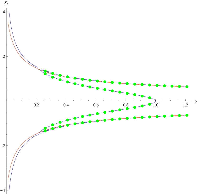
Figure 1: $H_{\mathrm{c}}$ and $S_{2\mathrm{c}}$ as function of $b$ ($\varepsilon=0.03$). Stable critical points are marked by (green) circle. Unstable critical points and points of complicated equilibrium are not shown in this figure. Solid lines in the left and right panel of figure correspond to solutions of eqs. (3.22) and (3.2) respectively.

4 Numerical integration of the system of gravitational equations

In this paper we will analyze the late time behaviour of the solution of the system (2.8)–(2.11). To make comparison with GR we will perform numerical integration of the system of the gravitational equations for dust matter ($w=0$). To simulate late-time behaviour the initial conditions will be taken at $t_{0}=0$ according to the following procedure.

1. For given value of $\varepsilon$ and $b$ ($\varepsilon>0$, $-\varepsilon+\sqrt{\varepsilon\left(2+\varepsilon\right)}<b<1$) algebraic system (3.17)–(3.18) is solved numerically and all critical points $P_{i}(H_{\mathrm{c}},S_{2\mathrm{c}},0,0)$ are found. Only real solutions are considered.

2. For every critical point, the stability analysis is carried out according to the previous subsection and stable point with minimal positive $H_{\mathrm{c}}$ and positive $S_{2\mathrm{c}}$ is selected.

3. The torsion function $S_{2}$ and the Hubble parameter $H$ can be represented in the form

   $$H^{2}=H_{\mathrm{c}}^{2}+y_{1}\,\rho,$$ (4.1)

   $$S_{2}^{2}=S_{2\mathrm{c}}^{2}+y_{2}\,\rho,$$ (4.2)

   with some coefficients $y_{1}$ and $y_{2}$. As the stable point is selected, then $\rho$ tends to zero at $t\to+\infty$. Keeping linear terms in $\rho$ the conservation law (2.11) can written as

   $$\rho^{\prime}=-3H_{\mathrm{c}}\rho.$$ (4.3)

   Substitution of (4.1)–(4.3) into (2.8)–(2) together with keeping terms linear in $\rho$ gives two algebraic equations for determination of $y_{1}$ and $y_{2}$. Numerical solution of these algebraic equations for given $\varepsilon$, $b$, $H_{\mathrm{c}}$ and $S_{2\mathrm{c}}$ gives $y_{1}$ and $y_{2}$.

4. Positivity of obtained values of $y_{1}$ and $y_{2}$ is considered as applicability of the late time approximation (4.1)–(4.2) and successful choice of stable critical point made in step 2 of current procedure. Further steps are performed only if $y_{1}>0$ and $y_{2}>0$.

5. Initial condition for $\rho_{0}=\rho(t_{0})$ is taken from the following equation

   $$\frac{H^{2}(t_{0})}{H_{\mathrm{c}}^{2}}\equiv\frac{H_{\mathrm{c}}^{2}+y_{1}\rho_{0}}{H_{\mathrm{c}}^{2}}=\frac{1}{\Omega_{\Lambda}},$$ (4.4)

   as result we have $H_{0}=H(t_{0})=\sqrt{H_{\mathrm{c}}^{2}+y_{1}\,\rho_{0}}$ and $S_{20}=S_{2}(t_{0})=\sqrt{S_{2\mathrm{c}}^{2}+y_{2}\,\rho_{0}}$. Here $\Omega_{\Lambda}$ is an additional free parameter that specifies initial conditions.

6. Initial condition for $S_{20}^{\prime}=S_{2}^{\prime}(t_{0})$ is obtained from (2.7) taking into account $k=0$. The minimal in modulus value of $S_{20}^{\prime}$ is taken as initial value.

7. For this choice of the parameters $\varepsilon$, $b$ and initial conditions $\rho_{0}$, $H_{0}$, $S_{20}$ and $S_{20}^{\prime}$ the system of differential equations (2.8)–(2.11) is integrated numerically.

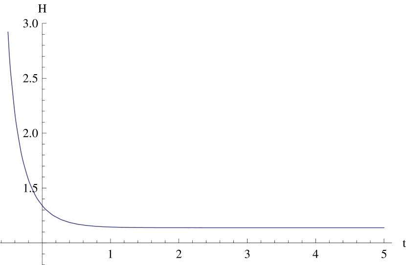
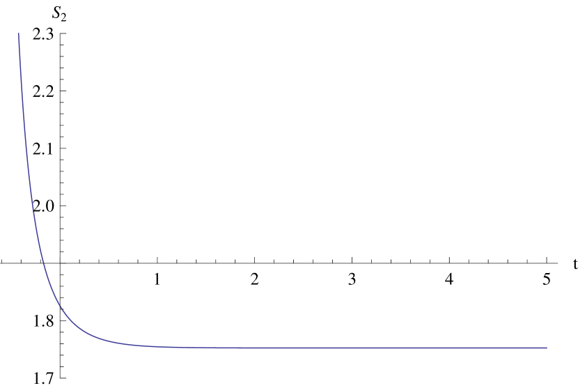
Figure 2: Late-time behaviour of Hubble parameter and $S_{2}$ torsion function.

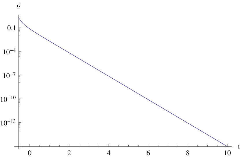
Figure 3: Late-time behaviour of the deceleration parameter and energy-density.

As an example let us consider the numerical solution at the following parameters and initial conditions $\varepsilon=0.00019$, $b=0.14$, $H_{0}=1.3417$, $S_{20}=1.82574$, $S^{\prime}_{20}=-0.288424$, $\rho_{0}=0.0730922$. This choice of the initial conditions gives $H^{2}(t_{0})/H^{2}(\infty)=1/\Omega_{\Lambda}=1/0{.}72$. Figures 2–3 show the behaviour of Hubble parameter $H$, torsion function $S_{2}$, deceleration parameter

$$q=-R^{\prime\prime}R/{R^{\prime}}^{2}$$ (4.5)

and energy-density of dust matter $\rho$. Another choice of the initial conditions leads generally speaking to cosmological solutions with another behaviour of the Hubble parameter and torsion function $S_{2}$ because of their oscillating character.

5 Comparison with observational data

In this Section we will analyze what restrictions on indefinite parameters leads to solutions corresponding to observational data. It should be noted that the numerical solution of gravitational equations allows to obtain time dependence of Hubble parameter $H(t)$ and scale factor $R(t)$ for given values of parameters of gravitational Lagrangian and initial conditions. As result dimensionless luminosity distance $\tilde{d}_{\mathrm{L}}$ can be obtained as a function of redshift $z$

$$z=\frac{R(t_{0})}{R(t)}-1=\frac{\tilde{R}(\tilde{t}_{0})}{\tilde{R}(\tilde{t})}-1$$ (5.1)

in the following form [30, 31]:

$$\tilde{d}_{\mathrm{L}}=\tilde{R}(\tilde{t}_{0})(1+z)\int_{\tilde{t}}^{\tilde{t}_{0}}\frac{d\tilde{t}}{\tilde{R}(\tilde{t})}=(1+z)\int_{0}^{z}\frac{dz}{\tilde{H}(z)}.$$ (5.2)

The predicted distance modulus $\mu=m-M$ ($m$ and $M$ are apparent and absolute magnitude respectively) can be written as function of dimensional luminosity distance $d_{\mathrm{L}}=\tilde{d}_{\mathrm{L}}\sqrt{6f_{0}\alpha}$ in the following form

$$\mu\equiv m-M=25+5\log_{10}d_{\mathrm{L}},$$ (5.3)

where $d_{\mathrm{L}}$ is given in megaparsecs.

5.1 Matching the late time approximation

At first we will compare late time approximation (4.1) of $H(t)$ with supernovae type Ia (SNe IA) observation data and predictions of the standard Big Bang Nucleosynthesis theory (BBN). Dependence of the energy density of the dust matter $\rho(t)\sim R^{3}(t)$ allows to write Hubble parameter in the late time approximation (4.1) as function of the redshift $z$. As result the corresponding expression for the predicted distance modulus $\mu$ takes the form

$$\mu(z)=25+5\log_{10}\left[\left(1+z\right)\int_{0}^{z}\frac{dz}{\sqrt{\Omega_{\Lambda}+\left(1-\Omega_{\Lambda}\right)\left(1+z\right)^{3}}}\right]+\mu_{0},$$ (5.4)

where

$$\mu_{0}=5\log_{10}\frac{\sqrt{6f_{0}\alpha}}{\tilde{H}_{0}\cdot\mathrm{1Mpc}}.$$

5.1.1 Comparison with SNe Ia observational data

We will start from comparison with supernovae observations using the Union2 compilation of 557 SNe Ia data [32] (see also [33]) and minimize

$$\chi_{\mathrm{SN}}^{2}=\sum_{i=1}^{557}\frac{\left[\mu(z_{i})-\mu_{\mathrm{obs}}(z_{i})\right]^{2}}{\sigma_{i}^{2}},$$ (5.5)

where $\sigma_{i}$ is the distance modulus errors.

Best fit parameters $\Omega_{\Lambda}=0.73$ and $\mu_{0}=18{.}16$ gives $\chi_{\mathrm{SN}}^{2}=542.683$ and $\chi_{\mathrm{SN}}^{2}/\mathrm{dof}=0.974$ (dof — degree of freedom). The value of $\mu_{0}=18{.}16$ corresponds to $70\,\mathrm{km}/(\mathrm{sec}\cdot\mathrm{Mpc})$ for Hubble constant at present epoch as in $\Lambda\mathrm{CDM}$-model of GR. Indeed, late time approximation (4.1) of $H(t)$ is similar to Friedmann equation of GR, but differs only by effective gravitational constant $G_{\mathrm{eff}}$ determined as $G_{\mathrm{eff}}=y_{1}G$.

If the matter content includes baryonic and dark matter with relative contributions $\Omega_{\mathrm{B}}$ and $\Omega_{\mathrm{DM}}$ to the total energy density, than it is easy to show [25] that

$$y_{1}=\frac{1-\Omega_{\mathrm{\Lambda}}}{\Omega_{\mathrm{DM}}+\Omega_{\mathrm{B}}}.$$ (5.6)

In particular, as matter candidate for cold dark matter is not found yet, it is possible to fit SNe Ia observational data in the discussed model without using dark matter ($\Omega_{\mathrm{DM}}=0$).

5.1.2 Comparison with SNe Ia + BBN data

Calculations in the frame of standard BBN theory predicts $\omega_{\mathrm{B}}\equiv\Omega_{\mathrm{B}}h^{2}=0.0212\pm 0.0010$ for baryon mass density [34], where $h$ is the Hubble constant at present epoch in units of $100\,\mathrm{km}/(\mathrm{sec}\,\mathrm{Mpc})$. For $h=0{.}7$ obtained earlier the corresponding $\Omega_{\mathrm{B}}=0{.}043$. Assuming that the rate of light element production during Big Bang Nucleosynthesis does not depend on the presence of the torsion and the dynamics of $H(t)$ from BBN epoch to present epoch is well approximated by (4.1), equation (5.6) gives $y_{1}=6{.}3$ for $\Omega_{\mathrm{\Lambda}}=0{.}73$ and $\Omega_{\mathrm{DM}}=0$. As $y_{1}$ is completely determined by parameters $b$ and $\varepsilon$, it seems impossible to determine $b$ and $\varepsilon$ simultaneously using late time approximation (4.1).

5.2 Matching general case

Besides approximation (4.1) there is another way to obtain the best fit parameters of considered theory. Namely, for given values of $\varepsilon$, $b$ and specified initial conditions, the procedure of numerical integration of exact system of differential equations (2.8)–(2.11) allows to obtain solution for $H(t)$, $\rho(t)$ and predicted distance modulus as a function of redshift $\mu=\mu(z)$. Obtained distance modulus - redshift dependence $\mu(z)$ allows to calculate joined $\chi^{2}$ for Union2 data set and BBN predictions

$$\chi^{2}=\chi_{\mathrm{SN}}^{2}+\chi_{\mathrm{BBN}}^{2},$$ (5.7)

where

$$\chi_{\mathrm{BBN}}^{2}=\frac{\left(\Omega_{\mathrm{B}}10^{-\bar{\mu}_{0}/5}c/\left(100\,\mathrm{km/sec}\right)-\omega_{\mathrm{B}}\right)^{2}}{\sigma_{y_{\mathrm{B}}}^{2}},$$

$c$ is the velocity of light and for computational purposes the functions $\mu(z)$ and $\Omega_{\mathrm{B}}$ are written in the following form

$$\mu(z)=25+5\log_{10}\left[\left(1+z\right)\int_{0}^{z}\frac{dz}{\tilde{H}(z)}\right]+\bar{\mu}_{0},$$ (5.8)

$$\bar{\mu}_{0}=5\log_{10}\frac{\sqrt{6f_{0}\alpha}}{\mathrm{1Mpc}},$$

$$\Omega_{\mathrm{B}}=\frac{1-\Omega_{\mathrm{\Lambda}}}{y_{1}}-\Omega_{\mathrm{DM}}.$$

According to [34] we will use $\omega_{\mathrm{B}}=0.0212$ and $\sigma_{y_{\mathrm{B}}}=0.0010$.

In general case $\chi^{2}$ depends on parameters $\alpha$, $b$, $\varepsilon$, initial conditions $\rho_{0}$, $H_{0}$, $S_{20}$, $S^{\prime}_{20}$ ($\Omega_{\Lambda}$) and cold dark matter contribution $\Omega_{\mathrm{DM}}$ to the total energy density. The task of minimization of total $\chi^{2}$ implies the minimization with respect to all parameters and initial conditions. To simplify this problem we will restrict the task by setting initial conditions in dependence on the values of parameters as was discussed in Section 4.

Following the previous subsection at first we will use the Union2 compilation set only. Considering the grid in the parameter region $0.00009\leq\varepsilon\leq 0.0002$, $0.12\leq\tilde{b}\leq 0.2$, $0.66\leq\Omega_{\Lambda}\leq 0.74$ ($\Delta\varepsilon=10^{-5}$, $\Delta\tilde{b}=0.01$, $\Delta\Omega_{\Lambda}=0.01$) and minimizing $\chi_{\mathrm{SN}}^{2}$ we find the minimum of $\chi_{\mathrm{SN}}^{2}$ at $\varepsilon\approx 0.00019$ and $\tilde{b}\approx 0.12$, $\Omega_{\Lambda}\approx 0.72$ and $\bar{\mu}_{0}=19.0074$ ($\chi_{\mathrm{SN}}^{2}=542.8$, $\chi_{\mathrm{SN}}^{2}/\mathrm{dof}=0.975$). Obtained values of parameters correspond to $70.0\,\mathrm{km}/(\mathrm{sec}\cdot\mathrm{Mpc})$ for Hubble constant at present epoch, $\omega_{\mathrm{B}}=0.0173$ and $\alpha^{-1}=4.22\cdot 10^{-30}\,\mathrm{g}/\mathrm{cm}^{3}$. Obtained value of $\omega_{\mathrm{B}}$ seems to be small and contradicts data on D- and ³He-abundance, but close to data on ⁴He [36].

Calculation $\chi^{2}$ defined by (5.7) in the same grid in parameter region $0.00009\leq\varepsilon\leq 0.0002$, $0.12\leq\tilde{b}\leq 0.2$, $0.66\leq\Omega_{\Lambda}\leq 0.74$ we find approximate best fit parameters for this model: $\varepsilon\approx 0.00019$, $\tilde{b}\approx 0.14$, $\Omega_{\Lambda}\approx 0.72$ and $\bar{\mu}_{0}=18.799$ ($\chi^{2}=542.9$, $\chi^{2}/\mathrm{dof}=0.983$). Obtained values of parameters correspond to $69.9\,\mathrm{km}/(\mathrm{sec}\cdot\mathrm{Mpc})$ for Hubble constant at present epoch, $\alpha^{-1}=5.11\cdot 10^{-30}\,\mathrm{g}/\mathrm{cm}^{3}$ and $\omega_{\mathrm{B}}=0.0198$ which is in accordance with data on ³He-abundance, and lies in $2\sigma$ interval for D-abundance. Solution presented in Figures 2–4 corresponds to this set of indefinite parameters. Comparison of the dependence of the distance modulus $\mu$ as a function of redshift $z$ for obtained numerical solution with that in $\mathrm{\Lambda CDM}$-model and Union2 observation data is presented in Figure 4.

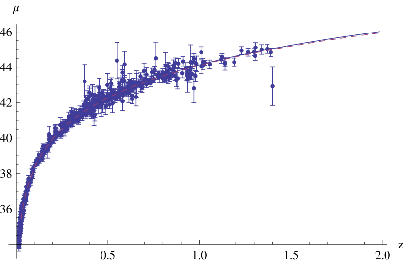
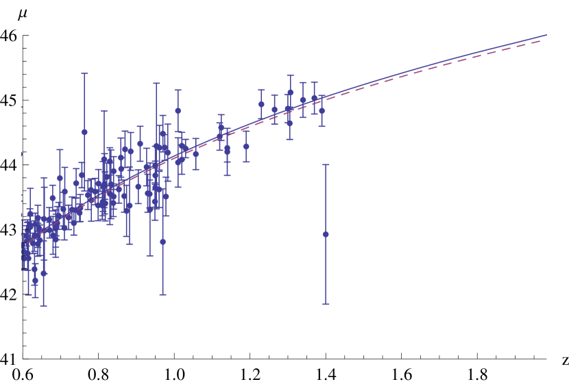
Figure 4: Comparison with SNe Ia observational data. Solid line corresponds to obtained numerical solution and dashed line corresponds to $\mathrm{\Lambda CDM}$-model.

6 Statefinder diagnostics

It was shown in a number of papers [37, 38] that so-called statefinder diagnostics proposed by Sahni, Saini, Starobinsky and Alam [39] allows to effectively discriminate between different models of dark matter and dark energy using the data from future SNAP-type satellite missions [40].

Statefinder diagnostics was applied to cosmology based on dynamic scalar torsion sector of PGTG [41] and it was found that some characteristics of the evolution of statefinder parameters

$$\bar{r}=R^{\prime\prime\prime}/RH^{3}\qquad\text{and}\qquad\bar{s}=(\bar{r}-1)/3(q-1/2)$$ (6.1)

can be distinguished from that for other cosmological models. The evolutionary trajectories of the statefinder pair ($\bar{r}$, $\bar{s}$) for numerical solution obtained in Section 4 are shown in the Figure 5 in the ($q$, $\bar{r}$) and ($\bar{s}$, $\bar{r}$) planes. This Figure demonstrates that statefinder diagnostics allows to distinguish cosmology in considered sector of PGTG from cosmology based on scalar torsion sector of PGTG [41] and other cosmological models, that allows in principle to differentiate the considered cosmological models from others using future SNAP-type satellite missions. It is necessary to note complicated and oscillatory behaviour of statefinder pair which is result of oscillating behaviour of the deceleration parameter (see Figure 3). As result the successful comparison observation data from planned SNAP-missions may require particular procedure for observation data processing.

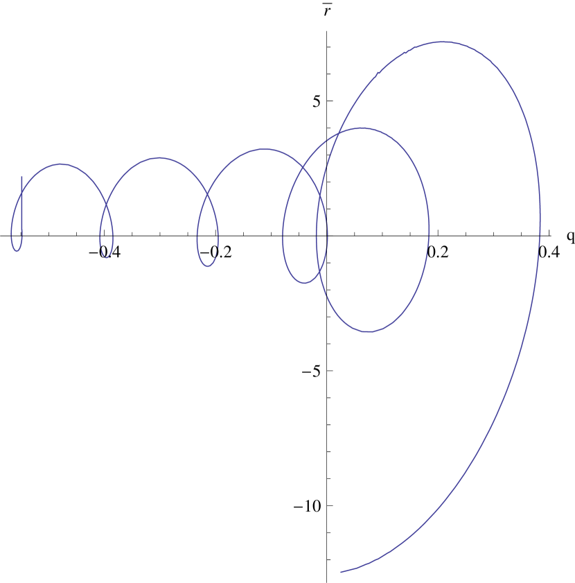
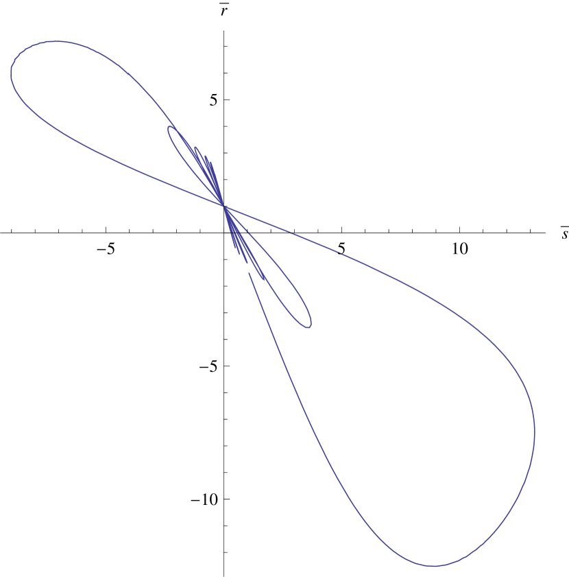
Figure 5: Evolutionary trajectories of statefinder pair

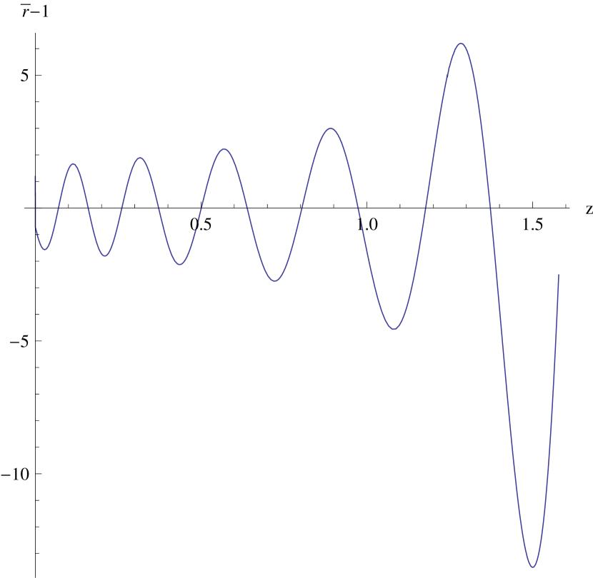
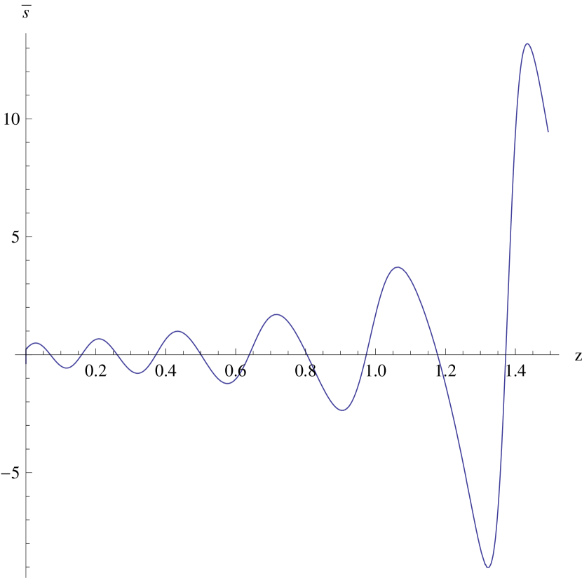
Figure 6: Statefinder pair as function of redshift $z$.

One of the possible procedure may consist in calculation of the statefinder pair ($\bar{r}$, $\bar{s}$) based on data from specially selected intervals ($z_{i}$, $z_{i+1}$). For example, averaging of the statefinder pair for the obtained numerical solution in the range $0.069\leq z\leq 0.26$ gives $\left<\bar{r}\right>=0.88$ and $\left<\bar{s}\right>=0.057$ which is close to that for $\mathrm{\Lambda CDM}$-model $(\bar{r},\,\bar{s})_{\mathrm{\Lambda CDM}}=(1,\,0)$, but averaging over intervals $0.069\leq z\leq 0.16$ and $0.16\leq z\leq 0.26$ gives $(\left<\bar{r}\right>,\,\left<\bar{s}\right>)$ equal to $(2.05,\,-0.36)$ and $(-0.15,\,0.43)$ correspondingly. Thus, averaging over twice smaller interval demonstrates different values and oscillations near the point $(1,\,0))$. This feature in the behaviour of the state finder pair can be used as a crucial test of the considered model in the planned SNAP-type satellite missions, but comprehensive analysis of possible tests of such type including the procedure of $z_{i}$ determination is out of this paper.

Conclusion

As follows from our analysis, homogeneous isotropic models built in the framework of the Poincaré gauge theory of gravity and filled by ideal fluid can have stable solutions with de Sitter asymptotics, if certain restrictions on indefinite parameters of the gravitational Lagrangian are imposed. Obtained model demonstrates accelerated expansion at the late time approximation and does not include dark energy for which physical nature is still unknown. Contribution of dark matter to the matter energy density is a free parameter of considered model and it can be either vanishing or non-vanishing. In the case of vanishing dark matter only baryonic matter with dust equation of state contributes to the total energy density in considered model.

Correspondence with SNe Ia observation data and BBN predictions are analyzed, where restricted set of indefinite parameters was considered and special procedure for determination of an initial conditions was used. Using this procedure best fit values of indefinite parameters and initial conditions are found. Obtained numerical solution was shown to be in a good correspondence with $\mathrm{\Lambda CDM}$-model as well as SNe Ia observation data and in an accordance with data on ³He- and D-abundance.

It was shown, that the trajectories of the statefinder pair for obtained solution demonstrate behaviour different from that in dynamic scalar torsion sector of PGTG and other cosmological models, that allows in principle to discriminate the considered cosmological models from others. Special feature in the behaviour of this trajectories is noticed allowing to test considered model using data from future SNAP-type satellite missions.

References

- [1] A.G. Riess et al., Observational Evidence from Supernovae for an Accelerating Universe and a Cosmological Constant, Astron. J. 116 (1998) 1009 [astro-ph/9805201].
- [2] S.J. Perlmutter et al., Measurements of and from 42 High-Redshift Supernovae, Astroph. J. 517 (1999) 565 [astro-ph/9812133].
- [3] J.A. Frieman, M.S. Turner, D. Huterer, Dark Energy and the Accelerating Universe, Ann.Rev.Astron.Astrophys. 466 (2008) 385 [arXiv:0803.0982].
- [4] V. Sahni, A. Starobinsky, Reconstructing Dark Energy, Int. J. Mod. Phys. D 15 (2006) 2105 [astro-ph/0610026].
- [5] T. Padmanabhan, Dark Energy: Mystery of the Millennium, AIP Conf.Proc. 861 (2006) 179 [astro-ph/0603114].
- [6] T.W.B Kibble, Lorentz Invariance and the Gravitational Field, J. Math. Phys. 2 (1961) 212.
- [7] A.M. Brodskii, D.D. Ivanenko, H.A. Sokolik, A New Conception of the Gravitational Field, Zhurnal Eksper. Theor. Fiz. 41 (1961) 1307.
- [8] D.W. Sciama, in Recent Developments in GR, Pergamon Press and PMN, Warsaw-New York (1962).
- [9] F.W. Hehl, P. von der Heyde, G.D. Kerlik, and J.M. Nester, General relativity with spin and torsion: Foundations and prospects, Rev. Mod. Phys. 48 (1976) 393.
-
[10]
K. Hayashi and T. Shirafuji, Gravity from Poincaré Gauge Theory of the Fundamental Particles. I — General Formulation,
Prog. Theor. Phys. 64 (1980) 866;
K. Hayashi and T. Shirafuji, Gravity from Poincaré Gauge Theory of the Fundamental Particles. II — Equations of Motion for Test Bodies and Various Limits, Prog. Theor. Phys. 64 (1980) 883;
K. Hayashi and T. Shirafuji, Gravity from Poincaré Gauge Theory of the Fundamental Particles. III — Weak Field Approximation, Prog. Theor. Phys. 64 (1980) 1435;
K. Hayashi and T. Shirafuji, Gravity from Poincaré Gauge Theory of the Fundamental Particles. IV — Mass and Energy of Particle Spectrum, Prog. Theor. Phys. 64 (1980) 2222. - [11] A.V. Minkevich, Gravitation, Cosmology and Space-Time Torsion, Ann. Fond. Louis de Broglie 32 (2007) 253 [arXiv:0709.4337].
- [12] A.V. Minkevich, Gravitational Interaction and Poincaré Gauge Theory of Gravity, Acta Physica Polonica B 40 (2009) 229 [arXiv:0808.0239].
- [13] A. Trautman, Einstein-Cartan theory, in: J.-P. Francoise, et al. (Eds.), Encyclopedia of Math. Physics, Elsevier, Oxford (2006), p.189 [gr-qc/0606062].
- [14] S. Capozziello, V.F. Cardone, E. Piedipalumbo, M. Sereno, A. Troisi, Matching torsion Lambda - term with observations, Int. J. Mod. Phys. D 12 (2003) 381 [astro-ph/0209610v1].
- [15] A.V. Minkevich, Generalised Cosmological Friedmann Equations without Gravitational Singularity, Phys.Lett. A 80 (1980) 232.
- [16] A.V. Minkevich, On Gravitational Repulsion Effect at Extreme Conditions in Gauge Theories of Gravity, Acta Physica Polonica B 38 (2007) 61 [gr-qc/0512123].
- [17] A.V. Minkevich, Gauge Approach to Gravitation and Regular Big Bang theory, Gravitation&Cosmology, 12 (2006) 11 [gr-qc/0506140].
- [18] A.V. Minkevich and A.S. Garkun, Analysis of inflationary cosmological models in gauge theories of gravitation, Class. Quantum Grav. 23 (2006) 4237 [gr-qc/0512130].
- [19] K.-F. Shie, J.M.Nester and H.-J. Yo, Torsion Cosmology and the Accelerating Universe, Phys. Rev. D78 023522 (2008) [arXiv:0805.3834].
- [20] H.Chen, F.-H. Ho, J.M.Nester, Ch.-H.Wang, H.-J. Yo, Cosmological dynamics with propagating Lorentz connection modes of spin zero, JCAP 0910 (2009) 027 [arXiv:0908.3323].
- [21] A.V. Minkevich, A.S. Garkun and V.I. Kudin, Regular accelerating Universe without dark energy in Poincaré gauge theory of gravity, Class. Quantum Grav. 24 (2007) 5835 [arXiv:0706.1157].
- [22] V.I. Kudin, A.V. Minkevich and F.I. Fedorov, On homogeneous isotropic cosmological models with torsion, Vestsi Akad. Navuk BSSR, ser. fiz.-mat. navuk, No 4 (1981) 59.
- [23] H. Goenner, F. Muller-Hoissen, Spatially homogeneous and isotropic spaces in theories of gravitation with torsion, Class. Quantum Grav. 1 (1984) 651.
- [24] A.V. Minkevich, De Sitter Spacetime with Torsion as Physical Spacetime in the Vacuum and Isotropic Cosmology, Mod. Phys. Lett. A 26 (2011) 259 [arXiv:1002.0538].
- [25] A.V. Minkevich, Accelerating Universe with spacetime torsion but without dark matter and dark energy, Phys. Lett. B. 678 (2009) 423 [arXiv:0902.2860].
- [26] A.S. Garkun, V.I. Kudin and A.V. Minkevich, Analysis of Regular Inflationary Cosmological Models with Two Torsion Functions in Poincaré Gauge Theory of Gravity, Int. J. Mod. Phys. A 25 (2010) 2005 [arXiv:0811.1430].
- [27] R. Agarwal, D. O‘Regan, An Introduction to Ordinary Differential Equations, Springer, New York (2008).
- [28] V.I. Arnol’d, Ordinary Differential Equations, Springer-Verlag, Berlin (1992).
- [29] D. Cox, J. Little, and D. O’Shea, Ideals, Varieties, and Algorithms, Springer, New York (2007).
- [30] S. Weinberg, Gravitation and Cosmology: Principles and Applications of the General Theory of Relativity, John Wiley & Sons, New York (1972).
- [31] A.G. Riess, et al., Type Ia Supernova Discoveries at z¿1 From the Hubble Space Telescope: Evidence for Past Deceleration and Constraints on Dark Energy Evolution, Astrophys. J. 607 (2004) 665 [astro-ph/0402512].
- [32] R. Amanullah et al., Spectra and Light Curves of Six Type Ia Supernovae at 0.511 ¡ z ¡ 1.12 and the Union2 Compilation, Astrophys. J. 716 (2010) 712 [arXiv:1004.1711].
- [33] M. Kowalski, et al., Improved Cosmological Constraints from New, Old and Combined Supernova Datasets, Astrophys. J. 686 (2008) 749 [arXiv:0804.4142].
- [34] G. Steigman, Primordial Nucleosynthesis: A Cosmological Probe, in Proc. of the IAU Symposium S268 (2010): Light Elements in the Universe, Cambridge Univ. Press, Vol. 5 19 [arXiv:0912.1114].
- [35] M. Brúggen, Effects of a torsion field on Big Bang nucleosynthesis, Gen.Rel.Grav. 31 (1999) 1935 [astro-ph/9906403].
- [36] G. Steigman, Primordial Nucleosynthesis in the Precision Cosmology Era, Ann. Rev. Nucl. Part. Sci. 57 (2007) 463 [arXiv:0712.1100].
- [37] U. Alam, V. Sahni, T.D. Saini and A.A. Starobinsky, Exploring the Expanding Universe and Dark Energy using the Statefinder Diagnostic, Mon. Not. Roy. Astron. Soc. 344 (2003) 1057 [astro-ph/0303009].
-
[38]
X. Zhang, Statefinder diagnosis in a non-flat universe and the holographic model
of dark energy, JCAP 0703 (2007) 007 [gr-qc/0611084];
B. Chang, H. Liu, L. Xu, C. Zhang and Y. Ping, Statefinder Parameters for Interacting Phantom Energy with Dark Matter, JCAP 0701 (2007) 016 [astro-ph/0612616];
D.J. Liu and W.Z.Liu, Statefinder diagnostic for cosmology with the abnormally weighting energy hypothesis, Phys. Rev. D 77 (2008) 027301 [arXiv:0711.4854]. - [39] V. Sahni, T.D. Saini, A.A. Starobinsky and U. Alam, Statefinder — a new geometrical diagnostic of dark energy, JETP Lett. 77 (2003) 201 [astro-ph/0201498].
- [40] G. Aldering (on behalf of the) SNAP collaboration, Overview of the SuperNova/Acceleration Probe (SNAP), LBNL-51191 [astro-ph/0209550].
- [41] X. Li, C. Sun, P. Xi, Statefinder diagnostic in a torsion cosmology, JCAP 0904 (2009) 015 [arXiv:0903.4724v1].
- [42] M. Visser, Jerk, snap and the cosmological equation of state, Class. Quantum Grav. 21 (2004) 2603 [gr-qc/0309109].