SIR EPIDEMICS ON A SCALE-FREE SPATIAL NESTED MODULAR NETWORK WITH NON-TRIVIAL THRESHOLD

Abstract. We propose a class of random scale-free spatial networks with nested community structures and analyze Reed-Frost epidemics with class related independent transmissions. We show that the epidemic threshold may be trivial or not depending on the relation among community sizes, distribution of the number of communities and transmission rates.

Keywords and phrases: Epidemics, SIR, Reed-Frost, percolation, long-range, directed, scale-free, modular, nested, communities, hierarchical, threshold, spatial.

2010 Mathematical Subject Classification:

Primary 60K35; 92D30.

Secondary 93A13; 82B43; 92C60.

1. Introduction

We consider a spatial random graph which at the same time is scale-free and has a nested community structure, and study Reed-Frost SIR epidemic ([20], [26]) on it. We find that with a natural transmission mechanism, in which transmissions occur independently with rates related to community sizes, the critical threshold is trivial or not depending on the relation between community sizes, distribution of number of communities to which each individual belongs and rate of the decay of the transmission probability as the community size increases. Scale-free networks ([7], [3], [14]) have been widely studied in the context of epidemics (see [29] and [11]) suggesting at first that this might lead to triviality of the critical threshold ([25], [18], [19], [35]). On the other hand, most scale-free networks lack a spatial dimensionality, which is quite relevant to make the models more realistic (see e.g. [10]): one of the few prosed networks possessing both features has been suggested by Yukich [34]. Yukich’s network is, however, missing network modularity, i.e. the gathering of individuals in communities with faster transmission rates (see [8], [9], [4], [5] and [6]), a feature which has gained recent interest due to its relevance in infectious transmission. The formation of communities can be described by several mechanisms, such as random intersection in which extra vertices randomly connect to the vertices of the graph and links are then generated between vertices connected to a common extra vertex (see [12] for a description of random intersection and a review of other mechanisms). However, most real community structures are nested (see, e.g., [31], [33] and [13]) unlike the networks generated by random intersection and similar mechanisms.

The class of random networks discussed here have spatial features, are scale-free and possess a nested community structure. The networks are based on a connectivity graph, which, for simplicity, is here taken to be $\mathbb{Z}^{d}$ endowed with a hierarchical structure of partitions into larger and larger communities. To generate the network each vertex $v\in\mathbb{Z}^{d}$ is assigned a random integer value $X_{v}$, where the $X_{v}$’s are i.i.d. random variables. Each vertex $v$ identifies an individual, which belongs to all communities up to level $X_{v}$ in the hierarchical structure. The basic random connectivity graph is obtained by adding to the nearest neighbor edges of $\mathbb{Z}^{d}$ all the edges between pairs of vertices belonging to at least one common community. For a wide class of distributions of the $X_{v}$’s the connectivity graph is scale-free.

We then consider Reed-Frost SIR epidemics on the connectivity network, in which infected individuals at time $t$ contact each neighbor independently with some transmission probability, and if the neighbor is susceptible it becomes infected. To complete the model, it is natural to consider basic transmission probabilities for nearest neighbor vertices, and then an additional probability, decreasing with the size of the community, of independent transmission for any community shared by two individuals. In this way, the transmission probabilities do not depend only from the connectivity graph, but directly from the shared classes, and give rise to a very realistic mechanism. The set of individuals ultimately affected by the Reed-Frost SIR epidemic is the set of vertices belonging to a percolation graph with connection probabilities given by the transmission probabilities ([22]); for natural choices of the probabilities of infection through shared communities the phase diagram of the percolation graph exhibits a transition from nontrivial to trivial percolation threshold.
In summary, the model depends on five parameters:

• $d$, indicating space dimension;

• $z$, determining the growth factor $z^{d}$ of community sizes;

• $\alpha\geq 1$, determining the distribution of the number of communities to which an individual belongs;

• $p$, indicating the transmission probabilities to neighbors;

• $\rho$, modulating the decrease in transmission probabilities for large communities.

Several random networks can be generated along the indicated lines. In particular, the construction must specify the form of each partition and the interconnections between partitions. To illustrate the mathematical properties of the networks, we discuss in Section 2 a very simple and schematic structure, in which at each level $k$ the space is partitioned into hypercubes of linear size $z^{k}$, which are then packed into hypercubes of linear size $z^{k+1}$ and so on. To keep things simple one can think to $z=2$. For simplicity, we also limit ourselves to just one single parameter $\alpha$ to generate the connectivity graph, although this is excessively simplified, as the inclusion in small communities is likely to follow a different pattern from that of inclusion in large communities. In Section 2 we give a detailed description of the construction of the connectivity network.

In Section 3 we show that the degree distribution $D_{v}$ of any vertex $v$ in the connectivity network satisfies

$$\lim_{h\rightarrow\infty}P(D_{v}\geq h)\ h^{-\gamma+1}\in\bigg{[}\frac{1}{2\alpha},\frac{d^{d/2+1}\omega_{d}}{d-\log_{z}\alpha}\bigg{]}$$

where $\omega_{d}$ is the volume of the $d$-dimensional unit ball and $\gamma-1=\frac{\log_{z}\alpha}{d-\log_{z}\alpha}$, so that the network is scale-free for all $\alpha\in(1,z^{d})$; in particular, for $z^{\frac{d}{2}}\leq\alpha\leq z^{\frac{2d}{3}}$ the network exhibits the typical value of $\gamma\in(2,3)$.

In Section 4 we complete the description of the Reed-Frost epidemic and begin the description of the phase diagram in the $\alpha-\rho$ variables; such description is completed in Section 5 by dominating the probability of transmission in certain sets by those in a long range percolation model extending a recent result in [23]; it is remarkable that although we use edge variables to bound a model based on site variables the result is still sharp and we identify the exact phase diagram.

1. For $\alpha\geq z^{d}$ the network has short range behavior, and the hierarchical communities structure is irrelevant for the existence of critical threshold: there is a critical epidemic threshold $p_{c}$ for all $\rho$.

2. For $1\leq\alpha<z^{d}$ the behavior depends on $\rho$: if $\rho<\frac{\alpha}{z^{d}}$ there is still a nontrivial epidemic critical threshold $p_{c}\in(0,1)$ while $p_{c}=0$ for $\rho>\frac{\alpha}{z^{d}}$. This means that percolation, and thus an infinite outbreak, occurs at all values of $p$ in the parameter range we just identified. In the scale-free region, determined by $\alpha\in(1,z^{d})$, $p_{c}$ is thus trivial or not depending on the transmission rate in large communities. It is trivial if the transmission rates are constant ($\rho=1$) or with a not too fast rate; on the other hand it is not trivial for $\rho$ below a critical curve in the phase diagram.

3. On the line $\alpha=1$ each vertex belongs to all communities: the model is similar to long-range percolation (see [28]) and is studied in [24]: $p_{c}=0$ or $p_{c}>0$ for the same parameter range as in long-range percolation.

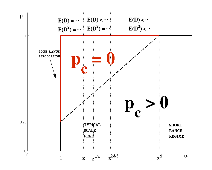
Figure 1. The phase space of the nested model in the $\alpha-\rho$ plane.

In a sense the proposed model interpolates between short ($\alpha\geq z^{d}$) and long ($\alpha=1$) range percolation. A summary of the phase diagram is in figure 1.

2. The connectivity graph

Consider a random graph $G_{\alpha,z}=(\mathbb{Z}^{d},E_{\alpha,z})$ with $\mathbb{Z}^{d}$ as set of vertices and a random set of edges $\mathbb{E}_{\alpha,z}$ to be specified. In the first place, $\mathbb{E}_{1}^{d}\subseteq E_{\alpha,z}$, where $\mathbb{E}_{1}^{d}$ is the set of nearest neighbor edges of $\mathbb{Z}^{d}$. Then, consider i.i.d. random variables $X_{v}$, $v\in\mathbb{Z}^{d}$, with a nonnegative integer distribution $\mu_{\alpha,v}$ such that $\mu_{\alpha,v}(X_{v}\geq k)=\alpha^{-k}$, $k=0,1,\dots$, where $\alpha>1$ is a parameter. We let $\mu_{\alpha}=\prod_{v\in\mathbb{Z}^{d}}\mu_{\alpha}$ the joint product distribution of the $X_{v}$’s on the Borel $\sigma$-algebra in $X=\mathbb{N}^{\mathbb{Z}^{d}}$. By this choice there is only one parameter determining the distribution of the number of communities to which individuals belong; the average number of communities to which an individual belongs, a measure called group membership (see [15] and [27]), is $\sum_{k}\alpha^{-d}=(\alpha-1)^{-1}$. This is a realistic number especially for $\alpha\in[5/4,2)$.

Next, let $z\geq 2$ be an integer and for each $k$ partition $\mathbb{Z}^{d}$ into blocks

$$B_{z,k}(i)=B_{z,k}(i_{1},\dots,i_{d})=\{v=(v_{1},\dots,v_{d})\in\mathbb{Z}^{d}:z^{k}i_{j}\leq v_{j}\leq(i_{j}+1)z^{k}-1,\text{ for all }j=1,\dots,d\}.$$

Blocks represent a system of nested communities. Note that vertices separated by coordinate hyperplanes lie always in different communities; the community structure is thus confined to orthants, and vertices in different orthants are connected only through nearest neighbor connections: this is not an unrealistic feature, however, as it might represent very rigid borders or seas.

Given $\rho_{\alpha}$ and the $B_{z,k}(i)$’s, the random connectivity graph $G_{\alpha,z}$ is completed by including into the edge set $E_{\alpha,z}$, next to the nearest neighbor edges, also all pairs $\{u,v\}$ such that $\exists k\in\mathbb{N},i\in\mathbb{Z}^{d}\textrm{ with }X_{u},X_{v}\geq k\textrm{ and }u,v\in B_{z,k}(i).$ In other words, given $\alpha$, $z$, $\mu_{\alpha}$ and $B_{z,k}(i)$’s, the random graph $G_{\alpha,z}$ is defined by a map $\phi_{z}:X\rightarrow H=\{0,1\}^{\mathbb{E}^{d}}$, where $\mathbb{E}^{d}=\{\{u,v\}:u,v\in\mathbb{Z}^{d}\}$, with

$$\phi_{z}(x)_{\{u,v\}}=\mathbb{I}_{\{\exists k\in\mathbb{N},\ i\in\mathbb{Z}^{d}|x_{u},x_{v}\geq k\textrm{ and }u,v\in B_{z,k}(i)\}}\vee\mathbb{I}_{\{|u-v|=1\}}$$

by $P_{\alpha,z}=\mu_{\alpha}(\phi_{z}^{-1})$. Later we are interested not only in the connectivity graph but also in the set of communities joining each pair of vertices: this leads to further specify the map $\phi_{z}$, as done in section $4$ below, but we first study the connectivity properties of $G_{\alpha,z}$.

For $v\in\mathbb{Z}^{d}$ and $\eta\in H$, let $D_{v}=D_{v}(\eta)=|\{u\in\mathbb{Z}^{d}:\{u,v\}\in\mathbb{E}_{\alpha,z}\}|$ be the degree of $v$.

Lemma 2.1.

For all $v\in\mathbb{Z}^{d}$ and $\alpha$, $z$ such that $\alpha<z^{d}$

(1) $$\lim_{h\rightarrow\infty}\mathbb{P}_{\alpha,z}(D_{v}\geq h)\cdot h^{\gamma-1}\geq\frac{1}{2\alpha},$$

where

$$\gamma-1=\frac{\log_{z}\alpha}{d-\log_{z}\alpha}$$

Proof.

Given $v\in\mathbb{Z}^{d}$ and $h\in\mathbb{N}$ consider the block $B_{z,l(h)}=B_{z,l(h)}(i)$ such that $v\in B_{z,l(h)}$ with $l(h)=\lfloor\frac{1}{d-\log_{z}\alpha}\log_{z}h+1\rfloor$. Then

$$\mathbb{E}_{\mu_{\alpha}}\bigg{(}\sum_{u\in B_{z,l(h)}}\mathbb{I}_{\{X_{u}\geq l(h)\}}\bigg{)} = z^{l(h)d}\mu_{\alpha}(X_{u}\geq l(h))$$

$$= \Big{(}\frac{z^{d}}{\alpha}\Big{)}^{l(h)}\ \geq\ \Big{(}\frac{z^{d}}{\alpha}\Big{)}^{\frac{\log_{z}\alpha}{d-\log_{z}\alpha}}\ =\ h.$$

By the CLT, $\lim_{h}\mu_{\alpha}(\sum_{u\in B_{z,l(h)}}\mathbb{I}_{\{X_{u}\geq l(h)\}}\geq h)\geq 1/2$. Hence,

$$h^{\gamma-1}\ \mathbb{P}_{\alpha,z}(D_{v}\geq h) \geq h^{\gamma-1}\ \mu_{\alpha}(X_{v}\geq l(h))\ \mathbb{P}_{\alpha,z}\bigg{(}\sum_{u\in B_{z,l(h)}}\mathbb{I}_{\{\{v,u\}\in E_{\alpha,d}\}}\geq h\ |\ X_{v}\geq l(h)\bigg{)}$$

$$\geq h^{\gamma-1}\ \alpha^{-l(h)}\ \mu_{\alpha}\bigg{(}\sum_{u\in B_{z,l(h)}}\mathbb{I}_{\{X_{u}\geq l(h)\}}\geq h\bigg{)}\rightarrow\frac{1}{2\alpha}$$

∎

To get the corresponding upper bound on the degree distribution we compare the connectivity graph to Yukich’s network, which has vertex heights based on uniform distributions and connections related to distance. As first step, we compare the connectivity graph to a network based only on distances but retaining the distribution of the $Z_{v}$’s for the vertex heights: for $\delta>0$ consider $G^{\prime}_{\alpha,z,\delta}=(\mathbb{Z}^{d},E^{\prime}_{\alpha,z,\delta})$ such that

(2) $$(u,v)\in E^{\prime}_{\alpha,z,\delta}\Leftrightarrow\exists k\textrm{ s.t. }X_{u},X_{v}\geq k\textrm{ and }d(u,v)\leq\delta z^{k};$$

more precisely, let $\phi_{z,\delta}^{\prime}:X\rightarrow H$ such that

(3) $$\phi_{z,\delta}^{\prime}(x)_{\{u,v\}}=\mathbb{I}_{\{\exists k\in\mathbb{N}\ |\ X_{u},X_{v}\geq k\textrm{ and }d(u,v)\leq\delta z^{k}\}}(x)$$

and let $P_{\alpha,z,\delta}^{\prime}=\mu_{\alpha}((\phi^{\prime}_{z,\delta})^{-1})$. Note that for $\delta=\sqrt{d}$ and for every increasing $A\subset H$

(4) $$\mathbb{P}_{z,\alpha}(A)\leq\mathbb{P}_{\alpha,z,\sqrt{d}}^{\prime}(A).$$

In fact, taking $k=\min(X_{u},X_{v})$, if $d(u,v)\geq\sqrt{d}\ z^{k}$ then $\{u,v\}\notin E_{\alpha,z}$. Therefore, if $\{u,v\}\in E_{\alpha,z}$ then $z^{k}\geq d(u,v)/\sqrt{d}$, so that $\{u,v\}\in E_{\alpha,z,\sqrt{d}}^{\prime}$, i.e. $\phi_{z}(x)\leq\phi^{\prime}_{z,\sqrt{d}}(x)$. This implies that if $A$ is increasing, $x\in X$ and $\phi_{z}(x)\in A$ then also $\phi^{\prime}_{z,\sqrt{d}}(x)\in A$, i.e. $(\phi_{z})^{-1}(A)\subseteq\Big{(}\phi^{\prime}_{z,\sqrt{d}}\Big{)}^{-1}(A).$

Note also that

(5) $$\phi_{z,\delta}^{\prime}(x)_{\{u,v\}}=\mathbb{I}_{\{z^{X_{u}},z^{X_{v}}\geq\frac{d(u,v)}{\delta}\}}(x).$$

3. Comparison with Yukich network

Let $\{U_{v}\}_{v\in\mathbb{Z}^{d}}$ be i.i.d. uniform $[0,1]$ random variables with distribution $P_{U}$ on $[0,1]^{\mathbb{Z}^{d}}$ and consider Yukich network $\bar{G}_{s,\delta}=(\mathbb{Z}^{d},\bar{E}_{s,\delta})$ defined for $s,\delta>0$ by

(6) $$\{u,v\}\in\bar{E}_{s,\delta}\ \Leftrightarrow\ d(u,v)\leq\delta\min(U_{u}^{-s},U_{v}^{-s})$$

As before one can take $W=[0,1]^{\mathbb{Z}^{d}}$, define $\bar{\phi}^{\prime}_{s,\delta}:W\rightarrow H$ such that

(7) $$\bar{\phi}^{\prime}_{s,\delta}(w)_{\{u,v\}}=\mathbb{I}_{\{w_{u},w_{v}\leq\frac{d(u,v)}{\delta}^{-1/s}\}}$$

and let $\mathbb{\bar{P}}^{\prime}_{s,\delta}=P_{U}((\bar{\phi}^{\prime}_{s,\delta})^{-1})$. We need to slightly reformulate Theorem 1.1 in Yukich ([34]) to incorporate the constant $\delta$.

Proposition 3.1.

For all $d,\delta$ and $s\in(\frac{1}{d},\infty)$

(8) $$\lim_{t\rightarrow\infty}t^{\frac{1}{sd-1}}\ \bar{\mathbb{P}}^{\prime}_{s,\delta}(D_{s}(v)\geq t)=\bigg{(}\frac{\delta^{d}sd\omega_{d}}{sd-1}\bigg{)}^{\frac{1}{sd-1}}$$

for all $v\in\mathbb{Z}^{d}$, where $\omega_{d}$ denotes the volume of the unit ball in $\mathbb{R}^{d}$.

Proof.

Yukich proves the same result for $\delta=1$. The conclusion is achieved by taking the origin $v=0$, conditioning on $U_{0}=\tau$ and using translation invariance. The basis of Yukich proof is Lemma 2.1 in [34], which states that

$$\mathbb{E}(D_{s}(0)|U_{0}=\tau)\approx\int_{|x|\leq\tau^{-s}}|x|^{-\frac{1}{s}}\ dx=d\omega_{d}\int_{0}^{\tau^{-s}}t^{d-1-\frac{1}{s}}\ dt=\frac{sd\omega_{d}}{sd-1}\ \tau^{-(sd-1)}$$

When a generic $\delta$ is considered we get

$$\mathbb{E}(D_{s}(0)|U_{0}=\tau) \approx \int_{|x|\leq\delta\tau^{-s}}|x|^{-\frac{1}{s}}\delta^{\frac{1}{s}}\ dx$$

$$= d\omega_{d}\delta^{\frac{1}{s}}\int_{0}^{\delta\tau^{-s}}t^{d-1-\frac{1}{s}}\ dt=\frac{\delta^{d}sd\omega_{d}}{sd-1}\ \tau^{-(sd-1)}$$

The rest of the proof in [34] is still valid with the constant $\beta=\frac{sd\omega_{d}}{sd-1}$ replaced by $\frac{\delta^{d}sd\omega_{d}}{sd-1}$ ∎

Then we can deduce the following upper bound for the power law distribution of the network $G_{\alpha,z}$.

Theorem 3.1.

For all $z$ and $\alpha\in(1,z^{d})$

(9) $$\lim_{h\rightarrow\infty}\mathbb{P}_{\alpha,z}(D(v)\geq h)\ h^{\gamma-1}\leq\bigg{(}\frac{d^{\frac{d}{2}+1}\omega_{d}}{d-\log_{z}\alpha}\bigg{)}^{\gamma-1}$$

where $\gamma-1=\frac{\log_{z}\alpha}{d-\log_{z}\alpha}$

Proof.

First recall that

(10) $$\mathbb{P}_{z,\alpha}(D\geq h)\leq\mathbb{P}_{z,\alpha,\sqrt{d}}^{\prime}(D\geq h)$$

since $\{D\geq h\}$ is increasing. We want to compare $G_{\alpha,z,\delta}^{\prime}$ to the Yukich’s network $\bar{G}^{\prime}_{s,\delta}$. For $m=z^{k}$

$$\mu_{\alpha}(z^{X_{v}}\geq m)=\mu_{\alpha}(X_{v}\geq k)=\alpha^{-k}=\alpha^{-\log_{z}m}=m^{-\log_{z}\alpha}.$$

On the other hand $P_{U}(U_{v}^{-s}\geq m)=P_{U}(U_{v}\leq m^{-1/s})=m^{-1/s}$ so that taking $\log_{z}\alpha=1/s$ we have

$$P_{U}(U_{v}^{-s}\geq m)=\mu_{\alpha}(z^{X_{v}}\geq m)\quad\text{ for }m=z^{k}$$

and

$$P_{U}(U_{v}^{-s}\geq m)=\alpha^{-\log_{z}m}\geq\alpha^{\lceil-\log_{z}m\rceil}=\mu_{\alpha}(X_{v}\geq\lceil\log_{z}m\rceil)=\mu_{\alpha}(X_{v}\geq\log_{z}m)=\mu_{\alpha}(z^{X_{v}}\geq m)$$

for all other $m\in\mathbb{R}$. Therefore, $U_{v}$ and $z^{X_{v}}$ can be coupled by the following joint distribution. Let $P_{U_{v}}$ be the distribution of $U_{v}$ and $\nu_{v}$ be a probability on the $\sigma$-algebra in $[0,1]\times\mathbb{N}$ such that for $A\subseteq[0,1]$ and $k\in\mathbb{N}$ it holds

$$\nu_{v}(A,k)=P_{U_{v}}\Big{(}A\cap(z^{-(k+1)/s},z^{-k/s}]\Big{)}.$$

We have

• $\nu_{v}(A,\mathbb{N})=P_{U_{v}}(A)$;

• $\nu_{v}([0,1],k)=P_{U_{v}}((z^{-(k+1)/s},z^{-(k)/s}])=\alpha^{-k}-\alpha^{-(k+1)}=\mu_{\alpha}(X_{v}=k);$

• $\nu_{v}\{(u,k):u^{-s}\geq z^{k}\}=\nu_{v}\{(u,k):u\leq z^{-k/s}\}=1$.

The product distributions $\mu_{\alpha}$ and $P_{U}$ can be coupled by the product distribution $\nu=\prod_{v\in\mathbb{Z}^{d}}\nu_{v}$, under which $U_{v}^{-s}\geq z^{X_{v}}$ for all $v\in\mathbb{Z}^{d}$ with probability one.
If $w\in W$ and $x\in\mathbb{N}^{\mathbb{Z}^{d}}$ are such that $w_{v}^{-s}\geq z^{x_{v}}$ for all $v$ then

$$\bar{\phi}^{\prime}_{s,\delta}(w)_{\{u,v\}} = \mathbb{I}_{\{w_{u}^{-1},w_{v}^{-1}\geq\frac{d(u,v)}{\delta}\}}$$

$$\geq \mathbb{I}_{\{z^{x_{u}},z^{x_{v}}\geq\frac{d(u,v)}{\delta}\}}=\phi^{\prime}_{z,\delta}(x)_{\{u,v\}}.$$

Thus, if $A\subseteq H$ is increasing, $x\in(\phi^{\prime}_{z,\delta})^{-1}(A)$ and $w_{v}^{-s}\geq z^{x_{v}}$ then $w\in(\bar{\phi}^{\prime}_{s,\delta})^{-1}(A)$. Hence, for $A$ increasing

$$P^{\prime}_{\alpha,z,\delta}(A) = \mu_{\alpha}\Big{(}(\phi^{\prime}_{z,\delta})^{-1}(A)\Big{)}$$

$$= \nu\Big{(}W,(\phi^{\prime}_{z,\delta})^{-1}(A)\Big{)}$$

$$= \nu\Big{(}(\bar{\phi}^{\prime}_{(\log_{z}\alpha)^{-1},\delta})^{-1}(A),(\phi^{\prime}_{z,\delta})^{-1}(A)\Big{)}$$

$$\leq \nu\Big{(}(\bar{\phi}^{\prime}_{(\log_{z}\alpha)^{-1},\delta})^{-1}(A),\mathbb{N}^{\mathbb{Z}^{d}}\Big{)}=P_{U}\Big{(}(\bar{\phi}^{\prime}_{(\log_{z}\alpha)^{-1},\delta})^{-1}(A)\Big{)}=\bar{P}^{\prime}_{(\log_{z}\alpha)^{-1},\delta}(A).$$

Since $A=\{D\geq h\}$ is increasing

$$P_{z,\alpha}(D\geq h)\leq P^{\prime}_{\alpha,z,\sqrt{d}}(D\geq h)\leq\bar{P}^{\prime}_{(\log_{z}\alpha)^{-1},\sqrt{d}}(D\geq h).$$

If we take $s=(\log_{z}\alpha)^{-1}$ and $\alpha\in(1,z^{d})$ then $s\in(1/d,\infty)$ and the result follows from Proposition 3.1 with $\delta=\sqrt{d}$. ∎

From lemma 2.1 and theorem 3.1, for large $h$ it holds $\mathbb{P}_{z,\alpha}(D=h)\approx h^{-\gamma}$ where $\gamma-1=\frac{\log_{z}\alpha}{d-\log_{z}\alpha}$.
Thus the hierarchical model is scale free for each $\alpha\in[1,z^{d})$. Typically, in the scale free region $-3\leq-\gamma\leq-2$, which is then equivalent to $z^{\frac{d}{2}}\leq\alpha\leq z^{\frac{2d}{3}}$.

We end this section by commenting on the relation between the scale free region and the average number of communities to which an individual belongs. As we have seen, there is a realistic average number of communities for $\alpha\in[5/4,2]$, which has no intersection with the typical scale-free region even for $d=2$ and $z=2$. It is, however, quite simple to realign the parameter ranges by introducing some more parameters more realistically describing small group membership. This is reminiscent of long range percolation in dimension 1, in which the probability of nearest neighbor connection can, by itself, determine phase transition for a critical value of the main parameter ([2]). We do not pursue this direction here.

4. Epidemics

We consider a Reed-Frost dynamics to describe the spread of an infection on the connectivity network (see, for instance, [12], section 3, for a detailed description). In such dynamics, at discrete times each infected individual contacts each one of its neighbors with some probability, and if the neighbor is susceptible it becomes infected; in the meantime the infected recovers. Differently from usual, we assume, however, that the probability of infectious contact depends on the communities shared by the two neighbors: in particular, we assume that there is a probability of independent transmission for each community shared by two individuals, and we are interested in the set of individual eventually affected by the epidemics started from one single vertex, the origin for instance. Such set can be identified with the cluster $V_{0}^{(d)}$ containing the origin in an edge percolation process on $G_{\alpha,z}$ described by the following probability measure: for each value $x\in\mathbb{R}^{d}$ of the $X_{v}$’s, consider a (conditional) Bernoulli probability distribution ${\mathbb{P}}_{x,z,\rho,p}$ on $\{0,1\}^{E_{x,z}}$ such that

(11) $${\mathbb{P}}_{x,z,\rho,p}(\eta_{\{u,v\}}=1)=1-\prod_{k=0}^{\infty}(1-p\rho^{k}\ \mathbb{I}_{\{\{u,v\}|\ \exists i\in\mathbb{Z}^{d}:\ x_{u},x_{v}\geq k\textrm{ and }u,v\in B_{k,z}(i)\}}).$$

Our main interest here is in studying for which values of the parameters there is a finite or an infinite set of infected individuals, or, equivalently, a finite or infinite cluster, i.e. we are interested in the probability $\mathbb{P}_{x,z,\rho,p}(|V^{(d)}_{0}|=\infty)$. The joint probability distribution which describes percolation and epidemics is defined on the Borel $\sigma$-algebra in $H$ by $\mathbb{P}_{\alpha,z,\rho,p}=\int_{X}\mathbb{P}_{x,z,\rho,p}\ \mu_{\alpha}(dx).$

For a given $x$ let $G_{x,z}$ be the realization of the connectivity graph with value $x$ of the $X_{v}$ variables. Since $G_{x,z}$ contains all the nearest neighbor edges and they are open with probability at least $p$, if $p>\pi_{c}^{(d)}$, the critical point for d-dimensional bond percolation, then percolation occurs regardless of the value of the other parameters and of the realization $x$. Notice that $\pi_{c}^{(d)}<1$ by Peierls argument, and, more precisely, $\pi_{c}^{(2)}=1/2$ ([17]) and $\pi_{c}^{(d)}\sim 1/2d$ ([21]). Moreover, for any fixed $x$ and $\rho$, the probability in (11) is increasing in $p$, and the random variables $\eta_{\{u,v\}}$ are independent. Thus, it follows by a standard FKG inequality (see, e.g., [16]) that for any $p\geq p^{\prime}$ and any increasing event $A\subseteq\{0,1\}^{E_{x,z}}$ we have ${\mathbb{P}}_{x,z,\rho,p}(A)\geq{\mathbb{P}}_{x,z,\rho,p^{\prime}}(A)$. Since $A^{(x)}_{0,\infty}=\{\eta:V^{(d)}_{0}|=\infty\}$ is increasing it follows that there exists a critical $p_{c}(x,\rho)<1$ for the onset of an infinite percolation cluster.

It could happen that $p_{c}(x,\rho)=0$. If $\alpha=1$ then we are assuming $X_{v}=\infty$ for all $v$, and the percolation model is quite close to long range percolation ([28]) in which the critical threshold $\pi_{c}$ has a transition at some value of a parameter which corresponds to $\rho$: for small values of $\rho$ we have $\pi_{c}>0$ and for large $\rho$ it is instead $\pi_{c}=0$. After showing that, in fact, the critical threshold $p_{c}(x,\rho)=0$ is almost surely constant in $x$, we see that a similar transition occurs in the hierarchical model for all values of $\alpha\in[1,z^{d}]$. To this purpose we introduce a more detailed description of the model: consider $\Sigma=\mathbb{N}^{\mathbb{Z}^{d}}\times\{0,1\}^{\mathbb{E}^{d}\times\mathbb{N}}$ and parameters $\alpha,\rho$ and $p$. Then take a Bernoulli probability distribution $\tilde{\mathbb{P}}_{\alpha,\rho,p}$ on the Borel $\sigma$-algebra $\mathcal{A}$ in $\Sigma$ such that

• $\tilde{P}_{\alpha,\rho,p}(\sigma_{v}\geq k)=\alpha^{-k}\text{ for all }v\in\mathbb{Z}^{d}$;

• $\tilde{P}_{\alpha,\rho,p}(\sigma_{\{u,v\},k}=1)=p\rho^{k}\text{ for all }\{u,v\}\in\mathbb{E}^{d}\text{ and }k\in\mathbb{N}$

One then retrieves the probability $P_{\alpha,z,\rho,p}$ by considering the map $\psi_{z}:\Sigma\rightarrow H$ such that

$$\psi_{z}=\mathbb{I}_{\{\exists k\in\mathbb{N},\ i\in\mathbb{Z}^{d}:\ u,v\in B_{z,k}(i);\ \sigma_{u},\sigma_{v}\geq k;\ \sigma_{(\{u,v\},k)}=1\}}$$

and observing that $P_{\alpha,z,\rho,p}=\tilde{P}_{\alpha,\rho,p}(\psi_{z}^{-1})$. Notice that while $\tilde{P}_{\alpha,\rho,p}$ is Bernoulli, the distribution $P_{\alpha,z,\rho,p}$ on $H$ is not independent since, for instance, if $u,u^{\prime}\in B_{z,k}(0)\setminus B_{z,k-1}(0)$ then $P_{\alpha,z,\rho,p}(\eta_{\{0,u^{\prime}\}}=1|\eta_{\{0,u\}}=1)=\alpha^{-k}\neq\alpha^{-2k}=P_{\alpha,z,\rho,p}(\eta_{\{0,u^{\prime}\}}=1)$. $P_{\alpha,z,\rho,p}$ is actually one-dependent. xxxx

Lemma 4.1.

$p_{c}(x,\rho)$ is almost everywhere constant in $x$

Proof.

Under $\tilde{P}_{\alpha,\rho,p}$ the variables $\sigma_{u}$’s and $\sigma_{(\{u,v\},k)}$’s are collectively independent. Consider the $\sigma$-algebra $\bar{\mathcal{A}}_{n}$ generated by the variables with index in $\{(v,\{v,u\},k):v\in([-n,n]^{d}\cap\mathbb{Z}^{d})^{c};\{u,v\}\in\mathbb{E}^{d},u,v\in([-n,n]^{d}\cap\mathbb{Z}^{d})^{c};k\geq n\}$; then ${\mathcal{A}}_{\infty}=\cap_{n}\bar{\mathcal{A}}_{n}$ is trivial under $\tilde{P}_{\alpha,\rho,p}$.
Since the event $A_{\infty}=\{\eta|\exists v\in\mathbb{Z}^{d}:|V_{v}^{(d)}|=\infty\text{ in }\eta\}$ is such that $\psi_{z}^{-1}(A_{\infty})\in\bar{\mathcal{A}}_{n}$ for all $n\in\mathbb{N}$, then $\psi_{z}^{-1}(A_{\infty})\in{\mathcal{A}}_{\infty}$ and $\tilde{P}_{\alpha,\rho,p}(\psi_{z}^{-1}(A_{\infty}))=0,1$. Thus, $A_{\infty}$ has probability zero or one for $P_{\alpha,z,\rho,p}$-a.a. $\eta\in H$. Hence, $P_{x,z,\rho,p}(A_{\infty})=0,1$ for $\mu_{\alpha}$-a.a. $x\in X$. Since $p_{c}(x,\rho)$ exists for all $x\in X$, it is $\mu_{\alpha}$ almost surely constant. ∎

We can define $p_{c}(\alpha,\rho)=\inf\{p:\tilde{\mathbb{P}}_{\alpha,\rho,p}(\psi_{z}^{-1}(A_{\infty}))=1\}$. We already know that $p_{c}(\alpha,\rho)<1$. We see now that $p_{c}(\alpha,\rho)=0$ when the transmission probabilities for large communities do not decrease fast enough.

Lemma 4.2.

For $\alpha\in[1,z^{d})$ and $\rho>\frac{\alpha}{z^{d}}$ we have $p_{c}=p_{c}(\alpha,\rho)=0$.

Proof.

The joint probability $\tilde{\mathbb{P}}_{\alpha,\rho,p}$ suggests several dynamic constructions of the epidemics together with the reference graph; one is the following. Starting from the origin $0$ consider the sequence of boxes $B_{z,k}=B_{z,k}(0)$, $k=1,\dots$ and sequentially generate the following variables:

• $\sigma_{0}$;

• $\sigma_{v},v\in B_{z,1}$;

• $\sigma_{\{0,v\},1},v\in B_{z,1}$;

• $\sigma_{v},v\in B_{z,k}\setminus B_{z,k-1}$;

• $\sigma_{\{v,u\},j},u,v\in B_{z,k-1}\setminus B_{z,k-2},j=1,\dots,k-1$;

• $\sigma_{\{v,u\},k},u\in B_{z,k-1},v\in B_{z,k}$;

• $\sigma_{\{u,v\},0}$ for all nearest neighbor pairs $\{u,v\}$.

Note that at every step only new $\sigma$ variables are generated, that the last step can be performed at any time, possibly subdivided in several steps, and that the procedure generates all relevant $\sigma$ variables in the positive orthant: in fact, if $v^{\prime},u^{\prime}\in B_{z,k}\setminus B_{z,k-1}$ then $\sigma_{\{v,u\},j}$ is generated at step $(((k+1)_{b})$ for $j=1,\dots,k$ and $(j_{c})$ for all $j\geq k+1$; if, instead, $v^{\prime}\in B_{z,k}\setminus B_{z,k-1}$ and $v^{\prime}\in B_{z,k+r}\setminus B_{z,k+r-1}$, $r\geq 1$, then $\sigma_{\{v,u\},j}$ for $j=1,\dots,k+r-1$ is not generated but it is also not relevant in the process and for $j\geq k+r$ is generated at step $(j_{c})$.

Following this construction we can show that for $\alpha\in[1,z^{d})$, $\rho>\frac{\alpha}{z^{d}}$ and any $p>0$ there is an infinite cluster. We generate a sequence $i_{k},k\in\mathbb{N}$, of vertices in $B_{z,k}\setminus B_{z,k-1}$ or empty sets with the following procedure, in which the definition of $i_{k}$ depends on $3$ events which may occur depending on the status of $i_{k-1}$:

• $\text{ if }\sigma_{0}\geq 1\textrm{ then }i_{0}=0,\text{ else }i_{0}=\emptyset$;

• if $i_{k-1}\in B_{z,k-1}\setminus B_{z,k-2}$ and $\exists v\in B_{z,k}\setminus B_{z,k-1}$ such that $\sigma_{v}\geq k+1\text{ and }\sigma_{\{i_{k-1},v\},k}=1$ then $i_{k}$ equals one of such vertices $v$ (the first in some fixed order);

• if $i_{k-1}\in B_{z,k-1}\setminus B_{z,k-2}$ and $\exists v\in B_{z,k}\setminus B_{z,k-1}:\sigma_{v}\geq k+1\text{ but for all such $v$'s }\sigma_{\{i_{k-1},v\},k}=0$ then $i_{k}$ equals one of vertices $v$ with the first two properties (the first in some fixed order);

• if $i_{k-1}\in B_{z,k-1}\setminus B_{z,k-2}$ and for all $v\in B_{z,k}\setminus B_{z,k-1}$ we have $\sigma_{v}<k+1$ then $i_{k}=\emptyset$;

• if $i_{k-1}=\emptyset$ and $\exists v\in B_{z,k}\setminus B_{z,k-1}:\sigma_{v}\geq k+1$ then $i_{k}$ equals one of such vertices $v$ (the first in some fixed order);

• if $i_{k-1}=\emptyset$ and for all $v\in B_{z,k}\setminus B_{z,k-1}$ we have $\sigma_{v}<k+1$ then $i_{k}=\emptyset$;

Given the vertices $i_{k}$’s we can define the events:

• $A_{k}=\{\exists v\in B_{z,k}\setminus B_{z,k-1}:\sigma_{v}\geq k+1,\sigma_{\{i_{k-1},v\},k}=1\}$

• $C_{k}=\{\exists v\in B_{z,k}\setminus B_{z,k-1}:\sigma_{v}\geq k+1\text{ but either }i_{k-1}=\emptyset\text{ or for all such $v$'s }\sigma_{\{i_{k-1},v\},k}=0\}$

• $E_{k}=\{\text{for all }v\in B_{z,k}\setminus B_{z,k-1}\text{ it holds }\sigma_{v}<k+1\}$

where clearly $A_{k}$ is not defined if $i_{k-1}=\emptyset$. Notice that all the events $A_{k},C_{k}$ and $E_{k}$ are defined in terms of the variables at steps $(k_{a})$ and $(k_{c})$ of the construction outlined above. This implies that such events are defined in terms of variables which, once $i_{k-1}$ is given, are independent from those involved in defining $A_{i},C_{i}$ and $E_{i}$ for $i=1,\dots,k-1$. Moreover, for each $k$ the three events form a partition of the probability space. Therefore, the sequence $Z_{k}=a_{k}(c_{k},e_{k}\text{ respectively })$ if $A_{k}(C_{k},E_{k}\text{ respectively })$ occurs, is a (non-homogeneous) Markov chain, whose transition matrix can be estimated in terms of the $\sigma$ variables. In fact,

(12) $$P(Z_{k}=a_{k}|Z_{k-1}=a_{k-1}) = 1-\Big{(}1-\frac{p\rho^{k}}{\alpha^{k+1}}\Big{)}^{z^{dk}-z^{d(k-1)}}\geq 1-e^{-\frac{p\rho^{k}(z^{dk}-z^{d(k-1)})}{\alpha^{k+1}}}$$

(13) $$P(Z_{k}=c_{k}|Z_{k-1}=e_{k-1}) = 1-\Big{(}1-\frac{1}{\alpha^{k+1}}\Big{)}^{z^{dk}-z^{d(k-1)}}\geq 1-e^{-\frac{(z^{dk}-z^{d(k-1)})}{\alpha^{k+1}}}$$

and all other conditional probabilities are smaller than $e^{-\frac{p\rho^{k}(z^{dk}-z^{d(k-1)})}{\alpha^{k+1}}}$ if $Z_{k-1}=a_{k-1}$ or $Z_{k-1}=c_{k-1}$ and smaller than $e^{-\frac{(z^{dk}-z^{d(k-1)})}{\alpha^{k+1}}}$ if $Z_{k-1}=e_{k-1}$.

We have

$$P(Z_{k}=e_{k})=\sum_{z=a_{k-1},c_{k-1},e_{k-1}}P(Z_{k}=e_{k}|Z_{k-1}=z)\ P(Z_{k-1}=z)\ \leq\ e^{-\frac{p\rho^{k}(z^{dk}-z^{d(k-1)})}{\alpha^{k+1}}}$$

and

$$P(Z_{k}=c_{k})=\sum_{z=a_{k-1},c_{k-1},e_{k-1}}P(Z_{k}=c_{k}|Z_{k-1}=z)\ P(Z_{k-1}=z)\leq 2\ e^{-\frac{p\rho^{k-1}(z^{d(k-1)}-z^{d(k-2)})}{\alpha^{k+1}}}$$

so that if $\rho>\alpha/z^{d}$

$$\sum_{k=1}^{\infty}P(Z_{k}=e_{k})<\infty,\quad\sum_{k=1}^{\infty}P(Z_{k}=c_{k})<\infty.$$

By the first Borel-Cantelli Lemma $E_{k}$ and $C_{k}$ occur only a finite number of times, so that with probability one the sequence terminates with one $C_{k}$ and then $A_{h}$ for $h>k$. In such case the vertex $i_{k}$ is connected to an infinite cluster containing all vertices $i_{h}$ for $h>k$. Since there are countably many vertices there must be one $k$ and one vertex $v\in B_{z,k}\setminus B_{z,k-1}$ which is starting vertex of an infinite cluster using edges in communities at level at least $k$ with probability $c_{1}>0$. Such vertex can be connected to the origin using nearest neighbor edges, which are independent from the previous construction as they were involved only in the last step of the dynamic joint generation of graph and epidemic, with some probability $c_{2}>0$. In the end, the probability of percolation from the origin is at least $c_{1}c_{2}>0$. ∎

5. Domination by long-range percolation

The description of the $\alpha-\rho$ phase diagram is completed by the following result.

Theorem 5.1.

For $\alpha>z^{d}$ or $\alpha\in[1,z^{d}]$ and $\rho<\alpha/z^{d}$ we have $p_{c}>0$.

This amounts to prove that, with the parameters $\alpha$ and $\rho$ in the indicated region, there exists $p>0$ such that percolation does not occur for that value of $p>0$. To show this, we actually bound the probability of existence of an infinite percolation cluster or infinite infected area in the nested model with that in a long-range percolation, for which it is easy to show that percolation does not occur for some values of the parameter by bounding it with a subcritical Galton-Watson process.
A long-range percolation model is defined as a probability on the Borel $\sigma$-algebra in $H$ such that $Q_{\beta,s}(\eta_{\{u,v\}}=1)=\frac{\beta}{(d(u,v))^{s}}$.

Theorem 5.2.

When $s=\log_{z}(\alpha/\rho)$ and $\beta^{\prime}=\frac{p}{1-\rho}(\frac{\alpha}{\rho})^{\frac{1}{2}\log_{z}d}$, it holds that

$$\mathbb{P}_{\alpha,z,\rho,p}(|V_{0}^{(d)}|=\infty)=\tilde{\mathbb{P}}_{\alpha,\rho,p}(\psi_{z}^{-1}(|V_{0}^{(d)}|=\infty))\leq Q_{\beta^{\prime},s}(|V_{0}^{(d)}|=\infty).$$

The main difficulty lies in the fact that in the nested hierarchical model the distribution on the edges is one dependent: we face this problem later on. Initially, we once again compare the percolation network to $G^{\prime}_{\alpha,z,\delta}$ endowed with slightly larger infection probabilities than in the nested model.
Let $u,v\in\mathbb{Z}^{d}$, define

$$k_{1,\delta}(u,v)=\lceil\log_{z}\frac{d(u,v)}{\delta}\rceil,$$

and consider a Bernoulli probability distribution $\tilde{\mathbb{P}^{\prime}}_{\alpha,z,\rho,p,\delta}$ on the Borel $\sigma$-algebra $\mathcal{A}$ in $\Sigma^{\prime}=\mathbb{R}^{\mathbb{Z}^{d}}\times\{0,1\}^{\mathbb{E}^{d}_{n}}$ such that

• $\tilde{\mathbb{P}^{\prime}}_{\alpha,\rho,p,\delta}\ (\sigma^{\prime}_{v}\geq k)=\alpha^{-k}\qquad\text{ for all }v\in\mathbb{Z}^{d}$;

• $\tilde{\mathbb{P}^{\prime}}_{\alpha,\rho,p,\delta}\ (\sigma^{\prime}_{\{u,v\}}=1)=\frac{p}{1-\rho}\ \rho^{k_{1,\delta}(u,v)}\qquad\text{ for all }\{u,v\}\in\mathbb{E}^{d}.$

Consider then the map $\psi^{\prime}_{z,\delta}:\Sigma^{\prime}\rightarrow\mathbb{E}^{d}$ such that

$$(\psi^{\prime}_{z,\delta}(\sigma^{\prime}))_{\{u,v\}}=\mathbb{I}_{\{\sigma^{\prime}_{u},\sigma^{\prime}_{v}\geq k_{1}(u,v);\ \sigma^{\prime}_{\{u,v\}}=1)\}}$$

Lemma 5.1.

For all increasing events $A\subseteq H$, $\tilde{\mathbb{P}}_{\alpha,\rho,p}(\psi_{z,\delta}^{-1}(A))\leq\tilde{\mathbb{P}^{\prime}}_{\alpha,z,\rho,p,\delta}((\psi^{\prime}_{z,\delta})^{-1}(A))$

Proof.

Consider the $\sigma$-algebra $\mathcal{A}_{X}$ generated by the variables $\sigma_{u},u\in\mathbb{Z}^{d}$, and let $\tilde{\mathbb{P}}_{x,\rho,p}=\tilde{\mathbb{P}}_{\alpha,\rho,p}(\cdot|x)$ and $\tilde{\mathbb{P}^{\prime}}_{x,\rho,p,\delta}$ be the conditional probabilities of $\tilde{\mathbb{P}}_{\alpha,\rho,p}$ and $\tilde{\mathbb{P}^{\prime}}_{\alpha,z,\rho,p,\delta}$, respectively, given $\mathcal{A}_{X}$. Notice that the conditional probabilities no longer depend on $\alpha$ and that $\tilde{\mathbb{P}}_{x,\rho,p}(\psi_{z}^{-1})$ and $\tilde{\mathbb{P}^{\prime}}_{x,z,\rho,p,\delta}((\psi^{\prime}_{z,\delta})^{-1})$ are Bernoulli distributions on (the Borel $\sigma$-algebra of) $H$ under which

$$\tilde{\mathbb{P}}_{x,\rho,p}\Big{(}\psi_{z}^{-1}(\sigma_{\{u,v\}}=1)\Big{)}=1-\prod_{k\in I_{x}(u,v)}(1-p\rho^{k})$$

where

$$I_{x}(u,v)=\{k|\ \exists i\in\mathbb{Z}^{d}:u,v\in B_{k,z}(i)\text{ and }x_{u},x_{v}\geq k\},$$

and

$$\tilde{\mathbb{P}^{\prime}}_{x,z,\rho,p,\delta}\ \Big{(}(\psi^{\prime}_{z,\delta})^{-1}(\sigma^{\prime}_{\{u,v\}}=1)\Big{)}=\frac{p}{1-\rho}\ \rho^{\log_{z}\frac{d(u,v)}{\delta}}$$

Note also that $I_{x}(u,v)\subset\{k_{1,\sqrt{d}}(u,v),k_{1,\sqrt{d}}(u,v)+1,\ldots,\min(x_{u},x_{v})\}$ so that

$$1-\prod_{k\in I_{x}(u,v)}(1-p\rho^{k}) \leq 1-\prod_{k\geq k_{1,\sqrt{d}}(u,v)}(1-p\rho^{k})$$

$$= p\sum_{k\geq{k_{1,\sqrt{d}}(u,v)}}\rho^{k}-p\sum_{h>k\geq{k_{1,\sqrt{d}}(u,v)}}\rho^{k+h}+\dots$$

$$\leq \frac{p}{1-\rho}\ \rho^{\log_{z}\frac{d(u,v)}{\sqrt{d}}}$$

since the series in the second line is alternating with decreasing coefficients. Therefore,

$$\tilde{\mathbb{P}}_{x,\rho,p}(\psi_{z}^{-1}(\sigma_{\{u,v\}}=1))\ \leq\ \tilde{\mathbb{P}^{\prime}}_{x,\rho,p,\sqrt{d}}\ ((\psi^{\prime}_{z})^{-1}(\sigma_{\{u,v\}}=1))$$

and $\tilde{\mathbb{P}^{\prime}}_{x,\rho,p,\sqrt{d}}\ ((\psi^{\prime}_{z})^{-1})$ dominates in the FKG sense $\tilde{\mathbb{P}}_{x,\rho,p}(\psi_{z}^{-1})$.

Therefore, if $A\subseteq H$ is increasing then

$$\tilde{\mathbb{P}}_{\alpha,\rho,p}(\psi_{z}^{-1}(A))=\int_{X}\tilde{\mathbb{P}}_{x,\rho,p}(\psi_{z}^{-1}(A))\ \mu_{\alpha}(dx)\leq\int_{X}\tilde{\mathbb{P}^{\prime}}_{x,z,\rho,p,\sqrt{d}}((\psi^{\prime}_{z,\sqrt{d}})^{-1}(A))\ \mu_{\alpha}(dx)=\tilde{\mathbb{P}^{\prime}}_{\alpha,\rho,p,\sqrt{d}}((\psi^{\prime}_{z})^{-1}(A))$$

∎

To compare the percolation network $\tilde{\mathbb{P}^{\prime}}_{\alpha,z,\rho,p,\sqrt{d}}((\psi^{\prime}_{z,\sqrt{d}})^{-1})$ with a long-range percolation network we are going to prove an analogue of Theorem 3.1 in [23]. In this direction there are two main problems. On one side, [23] applies to directed paths; on the other side, connectivities in [23] are described by convex functions $k(X_{v},X_{u})$ and for values of $X_{u}=x_{u}$ the connectivities are bounded by expected values $\bar{x}_{v}=E(k(X_{v},x_{u}))$. In that paper the reason why the connections become independent in different directions is that the $\bar{x}_{v}$’s are constant.

The directionality of the paths is easy to fix: paths under $\tilde{P}^{\prime}_{\alpha,z,\rho,p}$ are not directed, but can trivially be considered so by fixing an order along each path. Paths are instead ordered under $\tilde{P^{\prime}}_{\alpha,\rho,p,\sqrt{d}}((\psi^{\prime}_{z})^{-1})$ since the involved edge variables are defined according to an order. Theorem 3.1 of [23] applies to hoppable collections of paths, such as the collection of all self-avoiding paths starting at the origin and reaching the boundary of some fixed set; since from each path one can extract a self-avoiding one, Theorem 3.1 applies to the occurrence of a connection from the origin to the boundary as well.

As to the connectivity functions, the analogous in the present context would be $k(X_{v},X_{u})=(\phi_{z}(X))_{\{v,u\}}$ which is not convex and cannot be easily related to any constant value. To proceed, we introduce families of i.i.d. random variables, one family for each $v\in\mathbb{Z}^{d}$, of the form $X^{\prime\prime}_{(v,u)},u\in\mathbb{Z}^{d}\setminus\{v\}$, and then bound $\tilde{\mathbb{P}^{\prime}}_{\alpha,z,\rho,p,\sqrt{d}}((\psi^{\prime}_{z})^{-1})$ by a network based on the $X^{\prime\prime}_{(v,u)}$’s. Connections in different directions are independent and depend only on distances, thus the network based on $X^{\prime\prime}_{(v,u)}$’s is actually a long-range percolation model. This is possible if we take the probability that $X^{\prime\prime}_{(v,u)}\geq k$ greater than or equal to the square root of the probability that $X^{\prime}_{v}\geq k$. This, in turn, implies that in the long-range model the presence of a vertex is equivalent, in distribution, to the fact that $X^{\prime}_{v}\geq k$ for one of its end-points, say the smallest in some fixed order. While this implies that the probability that the infection travels a self-avoiding path is larger in the long-range model, Theorem 5.4 below shows the same inequality holds for the probability that at least one paths is travelled among those in a fixed suitable collection.

Consider $\beta>0$ and a Bernoulli probability distribution $\tilde{\mathbb{P}^{\prime\prime}}_{\beta,z,\rho,p,\delta}$ on the Borel $\sigma$-algebra $\mathcal{A}$ in $\Sigma^{\prime\prime}=\mathbb{N}^{\mathbb{Z}^{d}\times\mathbb{Z}^{d}\setminus\{(i,i),i\in\mathbb{Z}^{d}\}}\times\{0,1\}^{E^{d}}$ such that

• $\tilde{\mathbb{P}^{\prime\prime}}_{\beta,z,\rho,p,\delta}(\sigma^{\prime\prime}_{(u,v)}\geq k)=\beta^{-k}\text{ for all }(u,v)\in\mathbb{Z}^{d}\times\mathbb{Z}^{d}\setminus\{(i,i),i\in\mathbb{Z}^{d}\}$;

• $\tilde{\mathbb{P}^{\prime\prime}}_{\beta,z,\rho,p,\delta}(\sigma^{\prime\prime}_{\{u,v\}}=1)=\frac{p\rho^{k_{1,\delta}(u,v)}}{1-\rho}\text{ for all }\{u,v\}\in\mathbb{E}^{d}.$

Consider then the map $\psi^{\prime\prime}_{z,\delta}:\Sigma^{\prime\prime}\rightarrow H$ such that

$$\psi^{\prime\prime}_{z,\delta}(\sigma^{\prime\prime})_{\{u,v\}}=\mathbb{I}_{\{\sigma^{\prime\prime}_{(u,v)},\ \sigma^{\prime\prime}_{(v,u)}\geq k_{1,\delta}(u,v);\ \sigma^{\prime\prime}_{\{u,v\}}=1\}}$$

and let $P^{\prime\prime}_{\beta,z,\rho,p,\delta}=\tilde{\mathbb{P}^{\prime\prime}}_{\beta,z,\rho,p,\delta}((\psi^{\prime\prime}_{z,\delta})^{-1})$. We denote by $\tilde{\mathbb{P}^{\prime\prime}}_{x^{\prime\prime},z,\rho,p,\delta}((\psi^{\prime\prime}_{z,\delta})^{-1})$ the conditional probability given $x^{\prime\prime}\in X^{\prime\prime}=\mathbb{N}^{\mathbb{Z}^{d}\times\mathbb{Z}^{d}\setminus\{(i,i),i\in\mathbb{Z}^{d}\}}$. Note that in passing from $\tilde{\mathbb{P}^{\prime}}_{\alpha,z,\rho,p,\delta}$ to $\tilde{\mathbb{P}^{\prime\prime}}_{\beta,z,\rho,p,\delta}$ we have changed the network mechanism and kept the same transmission rates.

We introduce an interpolation between $\tilde{\mathbb{P}^{\prime}}_{\alpha,z,\rho,p,\delta}$ and $\tilde{\mathbb{P}^{\prime\prime}}_{\beta,z,\rho,p,\delta}$. To this purpose we select an ordering of $\mathbb{Z}^{d}=\{v_{1},v_{2},\dots\}$ and, for $h=0,1,\dots$, we consider the sequence of sets $V(0)=\emptyset,\dots,V(h)=\{v_{1},\dots,v_{h}\}$. For later purposes we take the order such that $V(n^{d})=B_{n}=[0,n-1]^{d}\cap\mathbb{Z}^{d}$. Then we take a sequence of Bernoulli distributions $\tilde{P}_{h}$ defined on the Borel $\sigma$-algebras $\mathcal{A}(h)$ of $\Sigma(h)=\mathbb{N}^{\mathbb{Z}^{d}\setminus V(h)}\times\mathbb{N}^{V(h)\times\mathbb{Z}^{d}\setminus\{(i,i),i\in\mathbb{Z}^{d}\}}\times\{0,1\}^{\mathbb{E}^{d}}$ by

$$\tilde{P}_{h}(\sigma_{v}\geq k) = \frac{1}{\alpha^{k}}\qquad v\in\mathbb{Z}^{d}\setminus V(h)$$

$$\tilde{P}_{h}(\sigma_{(v,u)}\geq k) = \frac{1}{\beta^{k}}\qquad v\in V(h),u\in\mathbb{Z}^{d}\setminus v$$

$$\tilde{P}_{h}(\sigma_{\{v,u\}}=1) = \frac{p}{1-\rho}\ \rho^{k_{1,\delta}(u,v)}$$

Furthermore, define the map $\psi_{z,h}:\Sigma(h)\rightarrow H$ given by

$$(\psi_{z,\delta,h}(\sigma))_{\{u,v\}}=\mathbb{I}_{\{\sigma_{t(v,u)}\geq k_{1,\delta}(u,v),\ \sigma_{t(u,v)}\geq k_{1,\delta}(u,v),\ \sigma_{\{u,v\}}=1\}}$$

where $t(u,v)=u$ if $u\in\mathbb{Z}^{d}\setminus V(h)$ and $t(u,v)=(u,v)$ if $u\in V(h)$. We have $\tilde{P}_{0}(\psi_{z,0}^{-1})=\tilde{P}^{\prime}_{\alpha,z,\rho,p,\delta}((\psi^{\prime}_{z})^{-1}).$

Fix now a box $B_{n}=[0,n-1]^{d}\cap\mathbb{Z}^{d}$ and consider the variables $\sigma|_{B_{n}}$, which are the $\sigma$’s restricted to $B_{n}$, i.e. to the index set $\{(v),(v,u),\{v,u\}:v,u\in B_{n}\}$. For $v,u\in B_{n}$ and $h\leq n^{d}$, $(\psi^{\prime\prime}_{z,\delta,h}(\sigma^{\prime\prime}))_{\{v,u\}}$ and $(\psi_{z,\delta}(\sigma))_{\{v,u\}}$ depend only from $\sigma^{\prime\prime}|_{B_{n}}$ and $\sigma|_{B_{n}}$, respectively. Therefore, $\tilde{P}_{n^{d}}(\psi^{-1}_{z,n^{d}})=\tilde{P^{\prime\prime}}_{\beta,z,\rho,p,\delta}((\psi^{\prime\prime})^{-1}_{z,\delta})$ by the definition of $\tilde{P}_{h}$.

Given a box $B_{n}\subseteq\mathbb{Z}^{d}$ and $v\in B_{n}$, let $E_{v,n}=\{\{v,u\}:u\in B_{n}\cap\mathbb{Z}^{d}\}$ and consider now a pair of (possibly empty) sets $A,B\subseteq E_{v,n}$, which in our case coincides with both $E^{\prime}_{v}$ and $E^{*}_{v}$ of [23], any $|A|$-dimensional vector $x=(x_{1},\dots,x_{|A|})\in(\mathbb{R}^{+})^{|A|}$ and any $|B|$-dimensional vector $y=(y_{1},\dots,y_{|B|})\in(\mathbb{R}^{+})^{|B|}$. For a fixed $h$, the values $x$ and $y$ are interpreted as realizations of $X_{u}$ if $u\in V(h)$ or $X_{(u,v)}$ if $u\notin V(h)$, respectively.

For $A\subseteq E_{v,n}$ we indicate by $Z_{A}$ the event $\{\eta:\eta_{\{v,u\}}=0\text{ for all }\{v,u\}\in A\}\subseteq H$ that none of the edges of $A$ is open, and for any probability $P$ on $H$ we define the zero functions $z_{v}(P;n;A,B;x,y)=P(Z_{A}\cup Z_{B})$ as the probability that either none of the edges of $A$ is open or none of the edges of $B$ is open; for any pair of probabilities $P^{(a)}$ and $P^{(b)}$ denote by $z_{v}(P^{(a)},n)\leq z_{v}(P^{(b)},n)$ the fact that $z_{v}(P^{(a)};n;A,B;x,y)\leq z_{v}(P^{(b)};n;A,B;x,y)$ for all pairs of disjoint and possibly empty sets of endpoints $A,B\subseteq E_{v,n}$, all $x\in\mathbb{R}^{|A|}$ and $y\in\mathbb{R}^{|B|}$. The extension of Theorem 3.1 in [23] that we are going to prove uses the following inequality.

Theorem 5.3.

If $\beta^{2}=\alpha$ then for all $n,h\in\mathbb{N}$ such that $v_{h}\in B_{n}$, $z_{v_{h}}(\tilde{P}_{h-1}(\tilde{\psi}_{z,\delta,h-1}^{-1}),n)\geq z_{v_{h}}(\tilde{P}_{h}(\tilde{\psi}_{z,\delta,h}^{-1}),n)$.

Proof.

For fixed $B_{n}\subset\mathbb{Z}^{d}$ and $v=v_{h}\in B_{n}$, notice that the events $\tilde{\psi}_{z,\delta,h}^{-1}(Z_{A})$ and $\tilde{\psi}_{z,\delta,h}^{-1}(Z_{B})$ are measurable with respect to the variables $\sigma_{v}$, $\sigma_{(v,u)}$ and $\sigma_{\{v,u\}}$ which are indexed in the set $Z_{v,n}=\{v\}\cup\{\{v,u\},u\in B_{n}\setminus\{v\}\}\cup\{(v,u),u\in B_{n}\setminus\{v\}\}$. Then let $A,B\subseteq E_{v,n}$, disjoint, with $|A|=r$ and $|B|=m$, and $x\in\mathbb{R}^{|A|}$ and $y\in\mathbb{R}^{|B|}$ be fixed; we identify each edge in $A$ or $B$ by its endpont different from $v$. We then let

(14) $$A\cup B=(u_{1},u_{2},\ldots,u_{m+r})$$

indicate the vertices wihch are endpoints (different from $v$) of edges in $A\cup B$, ordered according to the distance of the endpoint from $v$, which is $d(v,u_{i})\leq d(v,u_{i+1})$. We also indicate $A=\{v_{1},v_{2},\ldots,v_{r}\}$ and $B=\{w_{1},w_{2},\ldots,w_{m}\}$. For simplicity of notation denote by $d_{u_{i}}=d(v,u_{i})$ the distance from $v$ to $u_{i}$ and by $\alpha_{u_{i}},\beta_{u_{i}}$ the following probabilities

(15) $$\alpha_{u_{i}} = \mu_{\alpha}\Big{(}X_{v}\geq\log_{z}\frac{d_{u_{i}}}{\sqrt{d}}\Big{)}=\alpha^{-\log_{z}(\frac{d_{u_{1}}}{\sqrt{d}})}$$

$$\beta_{u_{i}} = \mu_{\beta}\Big{(}X_{v,u_{i}}\geq\log_{z}\frac{d_{u_{i}}}{\sqrt{d}}\Big{)}=\beta^{-\log_{z}(\frac{d_{u_{1}}}{\sqrt{d}})}$$

Thus $\alpha_{v_{i}}=(\beta_{v_{i}})^{2}$. Furthermore, let $q_{u_{i}}=\frac{p\rho^{k_{1,\delta}(v,u_{i})}}{1-\rho}$ and $\mathbb{P}_{1}=\tilde{P}_{h-1}$ and $\mathbb{P}_{2}=\tilde{P}_{h}$; we want to prove that

(16) $$\mathbb{P}_{1}(Z_{A}\cup Z_{B})\geq\mathbb{P}_{2}(Z_{A}\cup Z_{B}).$$

Let’s proceed by induction on the cardinality of $A$ and $B$. Note that if $|A|=0$ or $|B|=0$ then $\mathbb{P}_{1}(Z_{A}\cup Z_{B})=\mathbb{P}_{2}(Z_{A}\cup Z_{B})=1$.

$(i)$ Suppose $A=\{u\}$, $B=\{w\}$. By symmetry we can assume that $d_{w}<d_{u}$; then $\alpha_{w}>\alpha_{u}$ and $\beta_{w}>\beta_{u}$. We have

$$\mathbb{P}_{1}(Z_{A}\cup Z_{B}) = 1-\mathbb{P}_{1}(Z_{A}^{c}\cap Z_{B}^{c})$$

$$= 1-\alpha_{u}q_{u}q_{w}$$

$$\mathbb{P}_{2}(Z_{A}\cup Z_{B}) = 1-\mathbb{P}_{2}(Z_{A}^{c}\cap Z_{B}^{c})$$

$$= 1-\mathbb{P}_{2}(Z_{A}^{c})\ \mathbb{P}_{2}(Z_{B}^{c})$$

$$= 1-\beta_{u}q_{u}\ \beta_{w}q_{w}$$

Since $\beta_{w}>\beta_{u}$ then $\beta_{u}\beta_{w}>\beta_{u}^{2}=\alpha_{u}$ and

$$\mathbb{P}_{1}(Z_{A}\cup Z_{B})\geq\mathbb{P}_{2}(Z_{A}\cup Z_{B})\quad\textrm{if }|A|=|B|=1.$$

In particular, equality holds if $d_{u}=d_{w}$.

$(ii)$ Now consider $\{u_{1},u_{2},\ldots u_{m+r}\}=\{v_{1},v_{2},\ldots v_{r}\}\cup\{w_{1},w_{2},\ldots w_{m}\}={A}\cup{B}$ such that $d_{u_{1}}\leq d_{u_{2}}\leq\ldots\leq d_{u_{m+r}}$. Note that for any probability $\mathbb{P}$

$$\mathbb{P}(Z_{A}\cup Z_{B})=\mathbb{P}(Z_{A})+\mathbb{P}(Z_{B})-\mathbb{P}(Z_{A}\cap Z_{B})$$

As before, consider the probability of $Z_{A}\cup Z_{B}$. With respect to $\mathbb{P}_{1}$, if $X_{v}<\log_{z}\frac{d_{v_{1}}}{\delta}$ then $Z_{A}$ occurs. Instead, if $\log_{z}\frac{d_{v_{i}}}{\delta}\leq X_{v}<\log_{z}\frac{d_{v_{i+1}}}{\delta}$ then there exist $i$ connections in the basic graph and $Z_{A}$ occurs if at least one of them is open. Thus

$$\mathbb{P}_{1}(Z_{A}) = (1-\alpha_{v_{1}})+\sum_{j=1}^{r-1}(\alpha_{v_{j}}-\alpha_{v_{j+1}})\prod_{i=1}^{j}(1-q_{v_{i}})+\alpha_{v_{n}}\prod_{i=1}^{r}(1-q_{v_{i}})$$

$$\mathbb{P}_{1}(Z_{B}) = (1-\alpha_{w_{1}})+\sum_{j=1}^{m-1}(\alpha_{w_{j}}-\alpha_{w_{j+1}})\prod_{i=1}^{j}(1-q_{w_{i}})+\alpha_{w_{m}}\prod_{i=1}^{m}(1-q_{w_{i}})$$

$$\mathbb{P}_{1}(Z_{A}\cap Z_{B}) = (1-\alpha_{u_{1}})+\sum_{j=1}^{r+m-1}(\alpha_{u_{j}}-\alpha_{u_{j+1}})\prod_{i=1}^{j}(1-q_{u_{i}})+\alpha_{u_{n+m}}\prod_{i=1}^{m+r}(1-q_{u_{i}}).$$

With respect to $\mathbb{P}_{2}$, since edges are open independently of each other, we have

$$\mathbb{P}_{2}(Z_{A}) = \prod_{i=1}^{r}(1-\beta_{v_{i}}q_{v_{i}})$$

$$\mathbb{P}_{2}(Z_{B}) = \prod_{i=1}^{m}(1-\beta_{w_{i}}q_{w_{i}})$$

$$\mathbb{P}_{2}(Z_{A}\cap Z_{B}) = \prod_{i=1}^{r}(1-\beta_{v_{i}}q_{v_{i}})\prod_{i=1}^{m}(1-\beta_{w_{i}}q_{w_{i}}).$$

We proceed by induction on $m+r$: we show that if (16) holds for $m+r-1$ then it holds also for $m+r$. The vertex $u_{m+r}$ can be either in $A$ or in $B$ and we assume with no loss of generality that $u_{m+r}=v_{r}\in A$. Then we show that if $\mathbb{P}_{1}(Z_{A^{\prime}}\cup Z_{B})\geq\mathbb{P}_{2}(Z_{A^{\prime}}\cup Z_{B})$ with $|A^{\prime}|=r-1$, $|B|=m$ then $\mathbb{P}_{1}(Z_{A}\cup Z_{B})\geq\mathbb{P}_{2}(Z_{A}\cup Z_{B})$ with $A=A^{\prime}\cup\{v\}$ and thus $|A|=r$, $|B|=m$. This is equivalent to show that

(17) $$\mathbb{P}_{1}(Z_{A}\cup Z_{B})-\mathbb{P}_{1}(Z_{A^{\prime}}\cup Z_{B})\geq\mathbb{P}_{2}(Z_{A}\cup Z_{B})-\mathbb{P}_{2}(Z_{A^{\prime}}\cup Z_{B}).$$

By elementary calculation it turns out that

$$\mathbb{P}_{1}(Z_{A})-\mathbb{P}_{1}(Z_{A^{\prime}})=-\alpha_{v_{n}}q_{v_{n}}\prod_{i=1}^{r-1}(1-q_{v_{i}})$$

$$\mathbb{P}_{1}(Z_{A}\cap Z_{B})-\mathbb{P}_{1}(Z_{A^{\prime}}\cap Z_{B})=-\alpha_{v_{r}}q_{v_{r}}\prod_{i=1}^{r-1}(1-q_{v_{i}})\prod_{j=1}^{m}(1-q_{w_{j}})$$

thus

$$\mathbb{P}_{1}(Z_{A}\cup Z_{B})-\mathbb{P}_{1}(Z_{A^{\prime}}\cup Z_{B})=-\alpha_{v_{r}}q_{v_{r}}\prod_{i=1}^{r-1}(1-q_{v_{i}})\bigg{[}1-\prod_{j=1}^{m}(1-q_{w_{j}})\bigg{]}$$

Similarly, with respect to $\mathbb{P}_{2}$ we have

$$\mathbb{P}_{2}(Z_{A})-\mathbb{P}_{2}(Z_{A^{\prime}})=-\beta_{v_{r}}q_{v_{r}}\prod_{i=1}^{r-1}(1-\beta_{v_{i}}q_{v_{i}})$$

$$\mathbb{P}_{2}(Z_{A}\cap Z_{B})-\mathbb{P}_{2}(Z_{A^{\prime}}\cap Z_{B})=-\beta_{v_{r}}q_{v_{r}}\prod_{i=1}^{r-1}(1-\beta_{v_{i}}q_{v_{i}})\prod_{j=1}^{m}(1-\beta_{w_{j}}q_{w_{j}})$$

so that

$$\mathbb{P}_{2}(Z_{A}\cup Z_{B})-\mathbb{P}_{2}(Z_{A^{\prime}}\cup Z_{B})=-\beta_{v_{r}}q_{v_{r}}\prod_{i=1}^{r-1}(1-\beta_{v_{i}}q_{v_{i}})\bigg{[}1-\prod_{j=1}^{m}(1-\beta_{w_{j}}q_{w_{j}})\bigg{]}$$

In order to prove inequality (17) we must show

$$-\alpha_{v_{r}}q_{v_{r}}\prod_{i=1}^{r-1}(1-q_{v_{i}})\bigg{[}1-\prod_{j=1}^{m}(1-q_{w_{j}})\bigg{]}\geq-\beta_{v_{r}}q_{v_{r}}\prod_{i=1}^{r-1}(1-\beta_{v_{i}}q_{v_{i}})\bigg{[}1-\prod_{j=1}^{m}(1-\beta_{w_{j}}q_{w_{j}})\bigg{]}$$

Since $\alpha_{v_{r}}=\beta_{v_{r}}^{2}$, this is equivalent to show that

$$\beta_{v_{r}}\prod_{i=1}^{r-1}(1-q_{v_{i}})\bigg{[}1-\prod_{j=1}^{m}(1-q_{w_{j}})\bigg{]}\leq\prod_{i=1}^{r-1}(1-\beta_{v_{i}}q_{v_{i}})\bigg{[}1-\prod_{j=1}^{m}(1-\beta_{w_{j}}q_{w_{j}})\bigg{]}$$

Since $\beta_{w_{i}}\leq 1$, $1-q_{w_{i}}\leq 1-\beta_{w_{i}}q_{w_{i}}$, thus

(18) $$\prod_{i=1}^{r-1}(1-q_{v_{i}})\leq\prod_{i=1}^{r-1}(1-\beta_{v_{i}}q_{v_{i}})$$

Moreover, we see now that

(19) $$\beta_{v_{r}}\bigg{[}1-\prod_{j=1}^{m}(1-q_{w_{j}})\bigg{]}\leq\bigg{[}1-\prod_{j=1}^{m}(1-\beta_{w_{j}}q_{w_{j}})\bigg{]}$$

proceeding by induction on $m$. If $m=1$ then

$$\beta_{v_{r}}q_{w}\leq\beta_{w}q_{w}$$

because $v_{r}$ is the vertex at maximal distance from $u$, so that $\beta_{v_{r}}\leq\beta_{w}$. Next we evaluate the increment between the $(m-1)$-th and $m$-th term.

$$\beta_{v_{r}}\bigg{[}1-\prod_{j=1}^{m}(1-q_{w_{j}})\bigg{]}-\beta_{v_{r}}\bigg{[}1-\prod_{j=1}^{m-1}(1-q_{w_{j}})\bigg{]} = \beta_{v_{r}}q_{w_{m}}\prod_{j=1}^{m-1}(1-q_{w_{j}})$$

$$\bigg{[}1-\prod_{j=1}^{m}(1-\beta_{w_{j}}q_{w_{j}})\bigg{]}-\bigg{[}1-\prod_{j=1}^{m-1}(1-\beta_{w_{j}}q_{w_{j}})\bigg{]} = \beta_{w_{m}}q_{w_{m}}\prod_{j=1}^{m-1}(1-\beta_{w_{j}}q_{w_{j}})$$

thus inequality (19) follows from inequality (18) and $\beta_{v_{n}}\leq\beta_{w_{m}}$. ∎

Now we are able to follow Meester and Trapman’s work [23] to bound from above the probability of large outbreak, i.e. the existence of an infinite open path, by the corresponding quantity in the long-range model. In order to prove the results below we need to recall some definitions; the detailed definitions are in [23]. An ordered set of edges in some $E\subseteq\mathbb{Z}^{d}\times\mathbb{Z}^{d}$ of the form $\xi=(v_{0}v_{1},v_{1}v_{2},\dots,v_{n-1}v_{n})$ is a (directed) path from $v_{0}$ to $v_{n}$. A path $\xi=(v_{0}v_{1},v_{1}v_{2},\dots,v_{n-1}v_{n},\dots)$ with infinitely many different edges is an infinite path. Given a finite or infinite path $\xi=(v_{0}v_{1},v_{1}v_{2},\dots,v_{n-1}v_{n})$ we indicate the truncation after $k$ edges as $\xi^{s}(k)=(v_{0}v_{1},v_{1}v_{2},\dots,v_{k-1}v_{k})$ and the tail starting after $k$ edges as $\xi^{t}(k)=(v_{k}v_{k+1},\dots)$; for two paths $\xi_{1}=(v_{0}v_{1},v_{1}v_{2},\dots,v_{n-1}v_{n})$ and $\xi_{2}=(v_{n}v_{n+1},\dots)$ we denote the conjunction by $(\xi_{1},\xi_{2})=(v_{0}v_{1},v_{1}v_{2},\dots,v_{n-1}v_{n},v_{n}v_{n+1},\dots)$. Next, let $\Xi$ be a collection of paths; if $E^{(n)}$ is the collection of the first $n$ edges of $E$ according to some given enumeration of $E$ then we indicate by $\Xi_{n}$ the set of finite paths of $\Xi$ all of which edges are in $E^{(n)}$ together with all the infinite paths of $\Xi$ truncated at the first instance they leave $E^{(n)}$.

Furthermore, given a configuration $\eta\in H=\{0,1\}^{E}$ we say that $\xi$ is open in $\eta$ if for all edges $\{v_{k},v_{k+1}\}$ we have $\eta_{\{v_{k},v_{k+1}\}}=1$. And we indicate by $C^{\Xi}$ the event that at least one path in $\Xi$ is open. We say that $\Xi$ is hoppable if

• for any $v\in\mathbb{Z}^{d}$ and any two paths $\xi$ and $\phi$ of $\Xi$ going through $v$, where $v$ is the end vertex of the $i$-th edge of $\xi$ and the starting vertex of the $j$-th edge of $\phi$, then $(\xi^{s}(i),\phi^{t}(j))\in\Xi$.

• $\lim_{n}C^{\Xi_{n}}=C^{\Xi}$

Theorem 5.4.

For every hoppable collection of paths $\Xi$ in $\mathbb{E}^{d}$

(20) $$\tilde{P^{\prime}}_{\alpha,z,\rho,p,\delta}((\psi^{\prime}_{z,\delta})^{-1}(C^{\Xi}))\leq\tilde{P}^{\prime\prime}_{\sqrt{\alpha},z,\rho,p,\delta}((\psi^{\prime\prime}_{z,\delta})^{-1}(C^{\Xi}))$$

Proof.

We mimic the proof of Theorem 3.1 of [23], dividing the argument into 3 steps. Since $\tilde{P^{\prime}}_{\alpha,z,\rho,p,\delta}$ and $\tilde{P}^{\prime\prime}_{\sqrt{\alpha},z,\rho,p,\delta}$ are not defined on the same space, we use the interpolating distributions $\tilde{P}_{h}$, which are such that two consecutive ones differ only in the variables related to a single vertex. Fix a box $B_{n}=[-n,n]^{d}\cap\mathbb{Z}^{d}$.

$(i)$ The first step is to show that for all $n$ and $h$ such that $v_{h}\in B_{n}$, $\tilde{P}_{h-1}(\psi^{-1}_{z,\delta,h-1}(C^{\Xi_{n}}))\leq\tilde{P}_{h}(\psi^{-1}_{z,\delta,h}(C^{\Xi_{n}}))$.

Since $\beta^{2}=\alpha$, by Theorem 5.3, $z_{v_{h}}(\tilde{P}_{h-1},n)\leq z_{v_{h}}(\tilde{P}_{h},n)$. Denote by $\Sigma^{\prime}(h)=\mathbb{N}^{\mathbb{Z}^{d}\setminus V(h)}\times\mathbb{N}^{(V(h)\setminus v_{h})\times\mathbb{Z}^{d}\setminus\{(i,i),i\in\mathbb{Z}^{d}\}}\times\{0,1\}^{\mathbb{E}^{d}\setminus E_{v,n}}=\mathbb{N}^{\mathbb{Z}^{d}\setminus(V(h)\cup v_{h})}\times\mathbb{N}^{(V(h-1))\times\mathbb{Z}^{d}\setminus\{(i,i),i\in\mathbb{Z}^{d}\}}\times\{0,1\}^{\mathbb{E}^{d}\setminus E_{v,n}}$; by $\Sigma_{n}^{\prime}(h)$ its restriction to $B_{n}$, and $\mathcal{A}^{\prime}_{h}$ and $\mathcal{A}^{\prime}_{h,n}$ the Borel $\sigma$-algebras generated by the variables in $\Sigma^{\prime}(h)$ and $\Sigma_{n}^{\prime}(h)$ respectively. For all $h$

$$\tilde{P}_{h}(\psi^{-1}_{z,\delta,h}(C^{\Xi_{n}})) = \int_{\Sigma_{n}^{\prime}(h)}\tilde{P}_{h}(\psi^{-1}_{z,\delta,h}(C^{\Xi_{n}})|\sigma^{\prime}_{\Sigma_{n}^{\prime}(h)})d\tilde{P}_{h}(\sigma^{\prime}_{\Sigma_{n}^{\prime}(h)})$$

$$= \int_{\Sigma_{n}^{\prime}(h)}\tilde{P}_{h,}(\psi^{-1}_{z,\delta,h}(C^{\Xi_{n}})|\sigma^{\prime}_{\Sigma_{n}^{\prime}(h)})d\tilde{P}_{h-1}(\sigma^{\prime}_{\Sigma_{n}^{\prime}(h)}),$$

where for $\sigma^{\prime}\in\Sigma_{n}^{\prime}(h)$, $P(\quad|\sigma^{\prime})$ is the conditional probability given $\mathcal{A}^{\prime}_{h,n}$; the last equality holds since $\tilde{P}_{h}$ coincides with $\tilde{P}_{h-1}$ on $\mathcal{A}^{\prime}_{h,n}$. Therefore,

$$\tilde{P}_{h}(\psi^{-1}_{z,\delta,h}(C^{\Xi_{n}})) - \tilde{P}_{h-1}(\psi^{-1}_{z,\delta,h-1}(C^{\Xi_{n}}))$$

$$= \int_{\Sigma_{n}^{\prime}(h)}(\tilde{P}_{h}(\psi^{-1}_{z,\delta,h}(C^{\Xi_{n}})|\sigma^{\prime}_{\Sigma_{n}^{\prime}(h)})-\tilde{P}_{h-1}(\psi^{-1}_{z,\delta,h-1}(C^{\Xi_{n}})|\sigma^{\prime}_{\Sigma_{n}^{\prime}(h)}))d\tilde{P}_{h-1}(\sigma^{\prime}_{\Sigma_{n}^{\prime}(h)}).$$

Now one can follow the proof of Theorem 3.1 in [23]: if the event $C^{\Xi_{n}}$ occurs in $\sigma^{\prime}_{\Sigma_{n}^{\prime}(h)}$ regardless of the variables in $Z_{V_{h},n}$, then the integrand is $0$. Otherwise, one can follow verbatim case 3. of the proof of Theorem 3.1 in [23] to conclude that $\tilde{P}_{h-1}(\psi^{-1}_{z,\delta,h-1}(C^{\Xi_{n}}|\sigma^{\prime}_{\Sigma_{n}^{\prime}(h)}))\leq\tilde{P}_{h}(\psi^{-1}_{z,\delta,h}(C^{\Xi_{n}}|\sigma^{\prime}_{\Sigma_{n}^{\prime}(h)}))$ for all $h=0,\dots,n^{d}-1$ and thus the unconditional inequality holds.

$(ii)$ By iteration,

$$\tilde{P^{\prime}}_{\alpha,z,\rho,p,\delta}((\psi^{\prime}_{z,\delta})^{-1}(C^{\Xi_{n}}))=\tilde{P}_{0}(\psi^{-1}_{z,\delta,0}(C^{\Xi_{n}}))\leq\tilde{P}_{n^{d}}(\psi^{-1}_{z,\delta,n^{d}}(C^{\Xi_{n}}))=\tilde{P^{\prime\prime}}_{\alpha,z,\rho,p,\delta}((\psi^{\prime\prime}_{z,\delta})^{-1}(C^{\Xi_{n}})).$$

$(iii)$ In the last step we consider a general hoppable collection of paths $\Xi$. By definition of hoppable collection of paths, since $C^{\Xi_{n}}$ is decreasing in $n$, it follows that

$$\tilde{P^{\prime}}_{\alpha,z,\rho,p,\delta}((\psi^{\prime}_{z,\delta})^{-1}(C^{\Xi})) = \lim_{n\rightarrow\infty}\tilde{P^{\prime}}_{\alpha,z,\rho,p,\delta}((\psi^{\prime}_{z,\delta})^{-1}(C^{\Xi_{n}}))$$

$$\tilde{P^{\prime\prime}}_{\alpha,z,\rho,p,\delta}((\psi^{\prime\prime}_{z,\delta})^{-1}(C^{\Xi})) = \lim_{n\rightarrow\infty}\tilde{P^{\prime\prime}}_{\alpha,z,\rho,p,\delta}((\psi^{\prime\prime}_{z,\delta})^{-1}(C^{\Xi_{n}}))$$

and using the previous steps the proof is completed. ∎

Proof.

(of Theorem 5.2). For all hoppable collections of paths $\Xi$, $C^{\Xi}$ is an increasing event in $H$; moreover, $\{|V_{0}^{(d)}|=\infty\}=C^{\Xi}$ when $\Xi$ is the collection of all infinite paths containing the origin. If $s=\log_{z}(\alpha/\rho)$ and $\beta^{\prime}=\frac{p}{1-\rho}(\frac{\alpha}{\rho})^{\frac{1}{2}\log_{z}d}$ then

$$\tilde{P}^{\prime\prime}_{\sqrt{\alpha},z,\rho,p,\delta}((\psi^{\prime\prime}_{z,\delta})^{-1}(\eta_{\{u,v\}}=1)) = \tilde{P}^{\prime\prime}_{\sqrt{\alpha},z,\rho,p,\delta}(\sigma_{(v,u)}\geq k_{1,\delta}(u,v),\ \sigma_{(u,v)}\geq k_{1,\delta}(u,v),\ \sigma^{\prime\prime}_{\{v,u\}}=1)$$

$$= (\sqrt{\alpha})^{-2k_{1,\delta}(u,v)}\frac{p\rho^{k_{1,\delta}(u,v)}}{1-\rho}$$

$$= \frac{p}{1-\rho}\Big{(}\frac{p}{\alpha}\Big{)}^{\lceil\log_{z}\frac{d(u,v)}{\sqrt{d}}\rceil}$$

$$\leq \frac{p}{1-\rho}\ \Big{(}\frac{\alpha}{\rho}\Big{)}^{\frac{\log_{z}{d}}{2}}\ d(u,v)^{-\log_{z}(\frac{\alpha}{\rho})}$$

$$= \frac{\beta^{\prime}}{(d(u,v))^{s}}=Q_{\beta^{\prime},s}(\eta_{\{u,v\}}=1)$$

for a long-range percolation model $Q_{\beta^{\prime},s}$. Combining Lemma 5.1 and Theorem 5.4, we have

$$P_{\alpha,z,\rho,p}(|V_{0}^{(d)}|=\infty) = \tilde{\mathbb{P}}_{\alpha,\rho,p}(\psi_{z}^{-1}(|V_{0}^{(d)}|=\infty))$$

$$\leq \tilde{\mathbb{P}^{\prime}}_{\alpha,z,\rho,p,\delta}((\psi^{\prime}_{z,\delta})^{-1}(|V_{0}^{(d)}|=\infty))$$

$$\leq \tilde{P}^{\prime\prime}_{\sqrt{\alpha},z,\rho,p,\delta}((\psi^{\prime\prime}_{z,\delta})^{-1}(|V_{0}^{(d)}|=\infty))$$

$$\leq Q_{\beta^{\prime},s}(|V_{0}^{(d)}|=\infty)$$

∎

Proof.

(of Theorem 5.1) In order to establish for which values of the parameters $\alpha,p,\rho,z$ no percolation occurs, it’s now sufficient to dominate the long-range percolation model $Q_{\beta^{\prime},s}$ by a subcritical Galton Watson tree. Recall that a GW tree is subcritical, i.e. the probability of extinction is one, if the expected value of the descendants of any vertex is less or equals to one. If $R_{v}$ denotes the number of neighbors of a vertex $v$ we have

$$E_{Q_{\beta^{\prime},s}}(R_{v})=2dp+\sum_{u\in\mathbb{Z}^{d}}\frac{p}{1-\rho}(\frac{\alpha}{\rho})^{\frac{\log_{z}{d}}{2}}\frac{1}{d(u,v)^{\log_{z}(\frac{\alpha}{\rho})}}\leq 2dp+\sum_{k\in\mathbb{N}}2dk^{d-1}\frac{p}{1-\rho}(\frac{\alpha}{\rho})^{\frac{\log_{z}{d}}{2}}\frac{1}{k^{\log_{z}(\frac{\alpha}{\rho})}}<\infty$$

for all $\rho\in[0,1]$ if $\alpha>z^{d}$ or for $\alpha\in[1,z^{d}]$ and $\rho<\frac{\alpha}{z^{d}}$. ∎

References

[1]
[2] Aizenman, M., Newman, C. (1986): Discontinuity of the percolation density in onedimensionalpercolation models. Comm. Math. Phys. 107 611 647.
[3] Albert, R., H. Jeong, and A.-L. Barabasi (1999): Diameter of the World Wide
Web. Nature 401, p.130.
[4] F. G. Ball, D. Mollison, G. Scalia-Tomba (1997) Epidemics with two levels of mixing, Ann.
Appl. Probab. 7 (1) 46-89.
[5] F. Ball, D. Sirl and P. Trapman (2009): Threshold behaviour and final outcome of an epidemic on a random network with household structure, Advances in Applied Probability 41 765-796.
[6] F. Ball, D. Sirl and P. Trapman (2010): Analysis of a Stochastic SIR epidemic on a random network incorporating household structure, Mathematical Biosciences 224(2), 53-73.
[7] Barab si, A.-L.; R. Albert (1999): Emergence of scaling in random networks. Science 286 509-512.
[8] R. Bartoszynski, On a certain model of an epidemic, Zastos. Mat. 13 (1972/73) 139-
151.
[9] N. G. Becker, K. Dietz, The effect of household distribution on transmission and
control of highly infectious diseases, Math. Biosci. 127 (1995) 207-219.
[10] Britton, T. (2005): Stochastic epidemic models: a survey, NY: Cambridge University Press.
[11]
T. Britton, S. Janson, and A. Martin-Löf (2007): Graphs with specified degree distributions, simple epidemics, and local vaccination strategies, Adv. in Appl. Probab., 39 (4), 922-948.
[12] Tom Britton, Maria Deijfen, Andreas N. Lager s, and Mathias Lindholm (2008): Epidemics on random graphs with tunable clustering. J. Appl. Probab. 45 , Number 3 , 743-756.
[13] Costello et al. (2009): Bacterial Community Variation in Human Body Habitats Across Space and Time. Science 326, 1694-1697
[14] Eriksen, K. A. and M. Hornquist (2001): Scale-free growing networks imply
linear preferential attachment. Phys. Rev. E
65.
[15] Glaeser, E. L., D. Laibson and B. Sacerdote. ”An Economic Approach To Social Capital,” Economic Journal, 2002, v112(483,Nov), 437-458
[16] Grimmett, G. R. (1999): Percolation. vol. 321 of
Grundlehren der Mathematischen Wissenschaften,
Springer-Verlag, Berlin, second ed.
[17] H. Kesten (1980), The critical probability of bond percolation on the square lattice equals 1/2, Comm. Math. Phys. 74, 41-59.
[18] Kephart J O, Sorkin G B, Chess D M, et al. (1997): Fighting Computer Viruses. Sci Am, 277, 56-61.
[19] Kephart J O, White S R, Chess (1993): Computers and epidemiology. IEEE Spectr, 30, 20-26.
[20] W. O. Kermack; A. G. McKendrick (1927) A Contribution to the Mathematical Theory of Epidemics, Proceedings of the Royal Society of London. Series A, 115, pp. 700-721
[21] H. Kesten (1982), Percolation theory for mathematicians, Progress in Probability and Statistics, vol. 2, Birkhauser, Boston, Mass.
[22] Kuulasmaa and S. Zachary (1984): On spatial general epidemics and
bond percolation processes. Journal of Applied Probability 21(4), 911-914.
[23] Meester, R., Trapman, P. (2010):
Bounding basic characteristics of spatial epidemics with a new
percolation model, Preprint.
[24]private communication.
[25] Moreno Y, G mez J B, Pacheco A F. (2003): Epidemic incidence in correlated complex networks. Phys. Rev. E
68.
[26] Neal, P. (2003): SIR epidemics on a Bernoulli random graph. J. Appl. Probab. Volume 40, Number 3, 779-782.
[27] M. E. J. Newman, The structure and function of complex networks, SIAM Review 45, 167-256 (2003)
[28]
Newman, C.M. and Schulman, L.S. (1986): One-dimensional 1/—j-i—s percolation models. Comm. Math. Phys. 104, pp. 547-571.
[29] Sander L.M.1; Warren C.P.; Sokolov I.M. (2003): Epidemics, disorder, and percolation. Physica A, 325, Number 1, 1-8(8)
[30] Schulman, L. S. (1983): Long range percolation in one dimension, J. Phys. A. Lett., 16, L639-L641.
[31] Stokols, D., Clitheroe, C.
(2010): Environmental Psychology, in Environmental Health: from
global to local, H. Frumkin ed., San Francisco,USA, John Wiley & Sons.
[32])Trapman, P. (2006): On Stochastic Models for the Spread of Infections. PhD thesis, Vrije
Univ. Amsterdam.
[33] John E. Tropman, John L. Erlich, Jack Rothman (2000): Tactics and Techniques of Community Intervention Wadsworth Publishing.