Distance determination for RAVE stars using stellar models III: The nature of the RAVE survey and Milky Way chemistry

We apply the method of Burnett & Binney (2010) for the determination of stellar distances and parameters to the internal catalogue of the Radial Velocity Experiment (Steinmetz et al. 2006). Subsamples of stars that either have Hipparcos parallaxes or belong to well-studied clusters, inspire confidence in the formal errors. Distances to dwarfs cooler than $\sim 6000\,$K appear to be unbiased, but those to hotter dwarfs tend to be too small by $\sim 10\%$ of the formal errors. Distances to giants tend to be too large by about the same amount. The median distance error in the whole sample of 216 000 stars is $28\%$ and the error distribution is similar for both giants and dwarfs. Roughly half the stars in the RAVE survey are giants. The giant fraction is largest at low latitudes and in directions towards the Galactic Centre. Near the plane the metallicity distribution is remarkably narrow and centred on $\hbox{[M/H]}=-0.04\,$dex; with increasing $|z|$ it broadens out and its median moves to $\hbox{[M/H]}\simeq-0.5$. Mean age as a function of distance from the Galactic centre and distance $|z|$ from the Galactic plane shows the anticipated increase in mean age with $|z|$.

1 Introduction

In recent years there have been significant advances in our knowledge of the Galaxy due to a number of large-scale surveys in complementary magnitude ranges. The Hipparcos mission (Perryman 1997) obtained astrometry of unprecedented precision for a sample of bright stars that was complete only down to $V\sim 8$, and at the other end of the scale we have the Sloan Digital Sky Survey (SDSS, York et al. 2000), going no brighter than around magnitude $r=14$ and significantly fainter than $r=18$ (Ivezić et al. 2001). The sizable gap between these two studies is filled by the Radial Velocity Experiment (RAVE, Steinmetz et al. 2006), focusing primarily on magnitudes in the range $9<I<13$. RAVE is still ongoing, and has provided a number of important results regarding the structure and kinematics of the Galaxy (see for example Smith et al. 2007, Seabroke et al. 2008, Munari et al. 2009, Siebert et al. 2008, Siebert et al. 2010).

One of the challenges thrown up by recent surveys, concentrating as they do on relatively distant stars, is that of distance estimation. The astrometric precision required to measure trigonometric parallaxes to these stars is not yet available, so we must rely on secondary methods for determining stellar distances. A useful step in this direction was taken by Breddels et al. (2010), who showed that RAVE data could be used to estimate the parameters and thus distances for objects in the second RAVE data release. Their technique was honed by Zwitter et al. (2010), who used spectrophotometric distances to characterise the RAVE survey. An alternative approach was developed by Burnett & Binney (2010) in which our prior knowledge of the Galaxy and stars is more systematically exploited. In this paper we apply this technique to $\sim 216\,000$ stars observed by RAVE.

We determine spectrophotometric distances in parallel with other stellar parameters, in particular metallicity, age and mass, so we are able to study how the giant/dwarf ratio and the distributions in age and metallicity vary in the region surveyed by RAVE. Previous applications of Bayesian inference to the determination of stellar parameters have focused on single parameters such as age (Jørgensen & Lindegren, 2005); to our knowledge, this is the first study to consider all parameters together.

In Section 2 we specify the data on which our distances are based, and in Section 3 we summarise the algorithm used to calculate distances. Section 4 tests the derived distances by comparing them with (i) Hipparcos parallaxes and (ii) established cluster distances. The comparison with Hipparcos parallaxes uncovers slight biases in the distances to hot dwarfs and giants, respectively. Section 4 tests the validity of the formal errors by (i) comparing distances to the same stars derived from independent spectra, and (ii) comparing our distances with those obtained by Zwitter et al. (2010). The algorithm determines probability distributions for several stellar parameters in addition to distance. In Section 5 we display the distribution of formal errors in metallicity, age and initial mass, in addition to those in distance. In Section 6 we use our distances to explore which regions of the Galaxy are probed by the RAVE survey, and indicate which regions are predominantly probed with dwarfs or giants. In Section 7 whether examine how how mean age and metallicity vary within the probed portion of the Galaxy. Section 8 sums up.

2 The input data

Since it first took data in 2003 March, the RAVE survey has taken in excess of 400 000 spectra with resolution $R\simeq 7500$. A sophisticated reduction pipeline is required to recover stellar parameters such as $T_{\rm eff}$, $\log g$ and [M/H] from this huge dataset. The data pipeline involves several parameters whose values have to be optimised. Unfortunately, the values that are optimum for one purpose are not optimum for another. In particular, we will see in §4.1 that the settings that are optimised for dwarfs are sub-optimal for giants, and vice versa, so in this work we use distinct implementations of the pipeline for stars which have $\log g$ greater than, or less than 3.5, with the split based on the value of $\log g$ returned by the version of the pipeline that is used for the high-gravity stars. This is the “VDR2” version of the pipeline, which was used for RAVE’s 2nd data release (Zwitter et al. 2008) and also to produce a much larger data set that was released to the collaboration in 2010 January. The low-gravity stars are processed with the “VDR3” version of the pipelines, which was used for RAVE’s 3rd data release (Siebert et al. 2011) and also to produce data released to the collaboration in 2010 July.

We consider only data for stars that have spectra with signal-to-noise ratio $S/N\geq 20$, 2MASS photometry with quoted error in $J-K$ less than $0.3$, and values from RAVE for $T_{\rm eff}$, $\log g$, $\hbox{[M/H]}_{\rm raw}$, and [$\alpha$/Fe]. These criteria yield data for $216\,064$ distinct objects. We have obtained distances and stellar parameters for these stars.

We neglect the effects of extinction by dust because (a) we use near-infrared data, (b) most of the sample lies at quite high Galactic latitude, and (c) we do not have a straightforward method of estimating the reddening of individual stars.

The metallicities given in the RAVE data releases can be refined using calibration coefficients determined by comparing the raw RAVE metallicities with those obtained from high-resolution spectroscopy of a subset of stars. Each version of the pipeline comes with a calibrations: for VDR2 we have (Zwitter et al., 2008)

$$\hbox{[M/H]}=0.938\hbox{[M/H]}_{\rm raw}+0.767[\alpha/\hbox{Fe}]-0.064\log g+0.404,$$

while for VDR3 we have (Siebert et al., 2011)

$$\hbox{[M/H]}=1.094\hbox{[M/H]}_{\rm raw}+1.21[\alpha/\hbox{Fe}]-0.711{T_{\rm eff}\over 5040\,{\rm K}}+0.763$$

In the rest of this paper, all input values of [M/H] are those obtained by using the appropriate calibration formula above.

The observational errors of each star depend on the star’s signal-to-noise ratio ($S/N$). From Fig. 19 of Zwitter et al. (2008) we take the errors on temperature, gravity and metallicity at $S/N=40$ to be

$$\sigma_{\log T} = 0.0434,$$ (1)

$$\sigma_{\log g} = \cases{0.5,&if ${T_{\rm eff}}<8\,000$\,K;\cr 0.25+0.436\log\left(\frac{{T_{\rm eff}}}{8\,000\,{\rm K}}\right),&otherwise;}$$ (2)

$$\sigma_{\rm[M/H]} = 1.07\log{T_{\rm eff}}-3.71.$$ (3)

In the great majority of cases these errors are significantly larger than those given in Table 4 of Siebert et al. (2011) because the latter are simply internal errors obtained from repeat observations of the same star. As will become apparent in Section 4.1, there is a substantial component of systematic error in the stellar parameters, arising from the way the observed spectra have been fitted to stellar templates. The results of Section 4.1 show that the errors estimates we use are broadly correct.

Four entries in Table 4 of Siebert et al. (2011) show errors in $\log g$ that are more than 25 percent larger than those we have assumed, all for values of $\log g=2$ or 2.5. In three of these cases the associated error in $T_{\rm eff}$ is slightly larger than the value we have assumed. If future versions of the pipeline clearly show significant increases in the errors at intermediate gravities, the errors used in the distance-finding algorithm should be modified accordingly.

We obtain the errors at other values $S/N\neq 40$ from the empirical scaling given by eqs. (22) and (23) of Zwitter et al. (2008). Errors on colour and magnitude were taken from the 2MASS measurements on a star-by-star basis. No allowance is made for the error in [$\alpha$/Fe].

We take $J$ and $K$ magnitudes from the 2MASS catalogue (Skrutskie et al. 2006), and we use the Padova isochrones (Bertelli et al. 2008) – these isochrones are the only widely available ones that reproduce the red clump effectively (Zwitter et al., 2010).

3 Theory

We begin by briefly recapping the formalism developed in Burnett & Binney (2010), where a method for estimating the value of, and error on, each star’s distance, metallicity, age and mass was presented – Pont & Eyer (2004) give a useful introduction to the general methodology. We take the relevant observables for each RAVE star to be the logarithm of effective temperature $T_{\rm eff}$ and surface gravity $g$, the calibrated metallicity [M/H], colour $J-K$ and apparent $J$-magnitude. We combine these into the vector of observables

$$\mathbf{y}=\left(\log T_{\rm eff},\log g,\hbox{[M/H]},J-K,J\right).$$ (4)

Each star is assumed to be characterised by a set of ‘intrinsic’ parameters: true metallicity $\hbox{[M/H]}_{\rm t}$, age $\tau$, initial mass ${\cal M}$ and heliocentric distance $s$, which together form a second vector

$$\mathbf{x}=\left(\hbox{[M/H]}_{\rm t},\log\tau,{\cal M},s\right).$$ (5)

We assume Gaussian observational errors on each component of $\mathbf{y}$, thus the measured values $\bar{\mathbf{y}}$ for a star have probability density function (pdf)

$$p(\bar{\mathbf{y}}\,|\,\mathbf{y}(\mathbf{x}),\bm{\sigma}_{y})=G(\bar{\mathbf{y}},\mathbf{y}(\mathbf{x}),\bm{\sigma}_{y}),$$ (6)

where $\mathbf{y}(\mathbf{x})$ represents the true observables corresponding to intrinsic stellar values $\mathbf{x}$, and for an $n$-tuple $\mathbf{w}$ $G$ is defined to be the multivariate Gaussian

$$G(\mathbf{w},\bm{\mu},\bm{\sigma})\equiv\prod_{i=1}^{n}\left(\sigma_{i}\sqrt{2\pi}\right)^{-1}\exp\left(-(w_{i}-\mu_{i})^{2}/2\sigma_{i}^{2}\right).$$ (7)

The pdf of a star’s intrinsic parameters $\mathbf{x}$ is then conditional upon its observed values $\bar{\mathbf{y}}$, the observational errors $\bm{\sigma}_{y}$ and the fact $S$ that the star is observed in the survey in question. We thus seek the posterior pdf $p(\mathbf{x}\,|\,\bar{\mathbf{y}},\bm{\sigma}_{y},S)$. It is shown in Burnett & Binney (2010) that the moments of this distribution are given by

$$\mathcal{I}_{ik}=\int{\rm{d}}^{4}\mathbf{x}\,x_{i}^{k}\,\phi(\mathbf{x})\,G(\bar{\mathbf{y}},\mathbf{y}(\mathbf{x}),\bm{\sigma}_{y})\,p(\mathbf{x}),$$ (8)

where $\phi(\mathbf{x})$ describes any part of the survey selection function that cannot be expressed as a function of $\bar{\mathbf{y}}$. This leads to a value for the expectation of each stellar parameter through

$$\left<x_{i}\right>=\frac{\mathcal{I}_{i1}}{\mathcal{I}_{i0}},$$ (9)

and an uncertainty defined by

$$\sigma_{i}=\sqrt{\left(\mathcal{I}_{i2}/\mathcal{I}_{i0}\right)-\left<x_{i}\right>^{2}}.$$ (10)

The data were analysed using the prior of Burnett & Binney (2010), namely a three-component Milky Way model of the form

$$p(\mathbf{x})=p({\cal M})\sum_{i=1}^{3}p_{i}(\hbox{[M/H]})\,p_{i}(\tau)\,p_{i}(\mathbf{r}),$$ (11)

where $i=1,2,3$ correspond to a thin disc, thick disc and stellar halo respectively. We assumed the same initial mass function (IMF) for all three components following Kroupa et al. (1993) and Aumer & Binney (2009), namely

$$p({\cal M})\propto\cases{{\cal M}^{-1.3}&if ${\cal M}<0.5\,$M${}_{\odot}$,\cr 0.536\,{\cal M}^{-2.2}&if $0.5\,$M${}_{\odot}\leqslant{\cal M}<1\,$M${}_{\odot}$,\cr 0.536\,{\cal M}^{-2.519}&otherwise.}$$ (12)

The star-formation rate within the thin disc is assumed to have declined exponentially with time constant $8.4\,\rm{Gyr}$ (Aumer & Binney, 2009). The ages of halo and thick-disc stars are uncertain. We merely assume that the ages of all halo stars exceed $10\,\rm{Gyr}$, while those of thick-disc stars exceed $8\,\rm{Gyr}$. Since the thick disc is generally thought to be younger than most of the halo, we further assume that no thick-disc star has an age in excess of $12\,\rm{Gyr}$. The three components are therefore:

Thin disc ($i=1$):

$$p_{1}(\hbox{[M/H]}) = G(\hbox{[M/H]},0,0.2),$$

$$p_{1}(\tau) \propto \exp(0.119\,\tau/\mbox{Gyr})\quad\mbox{for $\tau\leqslant 10$\,Gyr,}$$ (13)

$$p_{1}(\mathbf{r}) \propto \exp\left(-\frac{R}{R_{\rm{d}}^{\rm{thin}}}-\frac{|z|}{z_{\rm{d}}^{\rm{thin}}}\right);$$

Thick disc ($i=2$):

$$p_{2}(\hbox{[M/H]}) = G(\hbox{[M/H]},-0.6,0.5),$$

$$p_{2}(\tau) \propto 8\leqslant\tau\leqslant 12$$ uniform in range  Gyr, (14)

$$p_{2}(\mathbf{r}) \propto \exp\left(-\frac{R}{R_{\rm{d}}^{\rm{thick}}}-\frac{|z|}{z_{\rm{d}}^{\rm{thick}}}\right);$$

Halo ($i=3$):

$$p_{3}(\hbox{[M/H]}) = G(\hbox{[M/H]},-1.6,0.5),$$

$$p_{3}(\tau) \propto 10\leqslant\tau\leqslant 13.7$$ uniform in range  Gyr, (15)

$$p_{3}(\mathbf{r}) \propto r^{-3.39}.$$

Here $R$ signifies Galactocentric cylindrical radius, $z$ cylindrical height and $r$ is spherical radius. The parameter values are given in Table 1.

Table 1: Values of disc parameters used.

Parameter	Value (pc)
$R_{\rm{d}}^{\rm{thin}}$	2 600
$z_{\rm{d}}^{\rm{thin}}$	300
$R_{\rm{d}}^{\rm{thick}}$	3 600
$z_{\rm{d}}^{\rm{thick}}$	900

4 Tests

In this section we show the results of a number of tests we performed to check the reliability and consistency of our stellar distances.

4.1 Hipparcos stars

Burnett & Binney (2010) demonstrated the robustness of the technique described in Section 3 on the Geneva-Copenhagen sample (Holmberg et al. 2009). However it is clearly important also to make sure that it functions correctly on the RAVE data. Consequently, we now investigate the performance of our method on the subset of RAVE stars that are in the Hipparcos catalogue, in its re-reduction by van Leeuwen (2007).

We identify RAVE stars that are in the Hipparcos Catalogue by requiring that sky positions (after updating the Hipparcos positions to J2000) coincide to $1.5\,$arcsec, and proper motions coincide to $2\sigma$, where $\sigma$ is the quadrature-sum of the errors in the proper motions in the RAVE and Hipparcos catalogues. This process leads to 4582 matches, but these matches include only 4080 distinct stars; the remaining matches arise from multiple RAVE observations of the same object.

  

  

Figure 1: Upper panels: distribution of normalized residuals (16) between our spectrophotometric parallaxes and values from Hipparcos. In this and subsequent histograms the quantity plotted vertically is the number of objects in the bin divided by the bin’s width, and an error bar shows the statistical uncertainty of each point. The mean and dispersion of each distribution are given at top right. A Gaussian of zero mean and unit dispersion is over-plotted. Lower panels: the distribution of fractional uncertainties in the spectrophotometric parallaxes. For the top panel the errors are found by adding our uncertainty and that of Hipparcos in quadrature; for the bottom panel the errors are just the spectrophotometric ones.

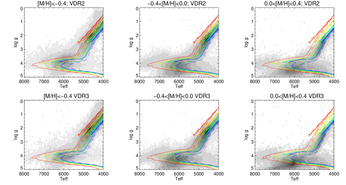
Figure 2: The density of RAVE stars with $S/N\geq 20$ in the $(T_{\rm eff},\log g)$ plane together with Padova isochrones for ages $3\,\rm{Gyr}$ (solid) and $9\,\rm{Gyr}$ (dashed). The colours indicate calibrated metallicities: $\hbox{[M/H]}=-1$ red; $\hbox{[M/H]}=-0.6$ yellow; $\hbox{[M/H]}=-0.2$ green; $\hbox{[M/H]}=0$ light blue; $\hbox{[M/H]}=0.1$ dark blue. The top row shows parameters from the VDR2 pipeline, while the lower row is for the VDR3 pipeline. In each row stars are grouped by metallicity, with the highest metallicities on the right. Note that in several panels, in the temperature range $6000\leq T_{\rm eff}\leq 7000$ the density of stars is high below the lowest isochrone. This anomaly is most pronounced in the lower row.

Given that the Bayesian method can output parallaxes as easily as distances, Burnett & Binney (2010) argued for comparisons with the Hipparcos data to be performed in parallax space. This is what we do in this section. It proves instructive to compare the stars in three groups: “giants” ($\log g<3.5$), “cool dwarfs” ($\log g\geq 3.5$ and $T_{\rm eff}<6000\,{\rm K}$) and “hot dwarfs” ($\log g\geq 3.5$ and $T_{\rm eff}\geq 6000\,{\rm K}$). Fig. 1 shows the normalised residuals

$$\mathcal{R}_{\varpi}\equiv\frac{\langle\varpi\rangle-\varpi_{\rm Hipparcos}}{\sqrt{\sigma_{\varpi}^{2}+\sigma_{\rm Hipparcos}^{2}}}$$ (16)

between the photometric and Hipparcos parallaxes for each of these groups. In each case the dispersion of the residuals is close to unity, which confirms the accuracy of the derived errors. For the cool dwarfs the mean residual is pleasingly close to zero, but the mean residual of the hot dwarfs is distinctly positive, indicating that the photometric parallaxes tend to be larger than the trigonometric ones. Fig. 2 makes the cause of this anomaly clear by showing the density of RAVE stars with $S/N\geq 20$ in the $(T_{\rm eff},\log g)$ plane together with isochrones for ages $3\,\rm{Gyr}$ (full) and $9\,\rm{Gyr}$ (broken) and metallicities ranging from $\hbox{[M/H]}=-1$ (red) to $\hbox{[M/H]}=0.1$ (dark blue). For $T_{\rm eff}\ga 6000\,{\rm K}$ and $\hbox{[M/H]}>-0.4$ there is a clear tendency for stars to be concentrated at higher values of $\log g$ than the isochrones allow. This shortcoming of the data fed to the Bayesian algorithm leads to the systematic under-estimation of the radii and therefore the luminosities of stars. Consequently, the predicted parallaxes are larger than they should be. Fig. 2 shows that the displacement of hot, relatively metal-rich stars to excessive values of $\log g$ is significantly more pronounced with the VDR3 pipeline (lower row) than with the VDR2 pipeline, and the stellar parameters from VDR3 yield a mean value of $\mathcal{R}_{\varpi}$ for the hot dwarfs which is as large as $0.273$.

The top right panel of Fig. 1 shows that the spectrophotometric parallaxes of giants are systematically too small, so $\mathcal{R}_{\varpi}=-0.11$. When the parameters output by the VDR2 pipeline are used for giants, we obtain $\mathcal{R}_{\varpi}=-0.19$. In fact, the VDR3 pipeline returns values of $\log g$ that are systematically larger than those returned by the VDR2 pipeline. For dwarfs the increases are relatively large and for many stars the VDR3 values are physically implausible. For giants the increases are smaller and seem to be beneficial.

The mean and dispersion displayed in Fig. 1 are for the distributions once we clip outliers, defined as stars with normalized residuals of modulus greater than four. This excludes eight stars of the original 4 080. Table 2 lists some data for these objects, one of which has repeat observations. It is notable that stars with $\log g<4$ are predicted to have smaller parallaxes than Hipparcos measured. For example, the $\log g$ value of Hipparcos 6075 is strongly indicative of a giant, so the stellar models predict for it an absolute $J$-magnitude in the range $M_{J}\in(-5.7,0.5)$; combined with its measured $\bar{J}=8.68$ this would imply a parallax in the range $\varpi\in(0.2,4.2)\,{\rm mas}$. Consequently the assignment of $\langle\varpi\rangle\in(0.42,1.04)\,{\rm mas}$ is eminently reasonable but in strong conflict with the Hipparcos value, $28.5\,{\rm mas}$. The Hipparcos magnitude of this star is three magnitudes fainter than its value of $\bar{J}$ from 2MASS. Either the star is exceptionally red, or the Hipparcos and 2MASS data relate to different objects.

Two of the stars with small $\log g$ and under-estimated parallax (Hipparcos 44216 and 46831) lie quite near the Galactic plane and may well be obscured, which would cause the predicted parallax to be too small. At www.rssd.esa.int/SA/HIPPARCOS/docs/vol11_all.pdf Hipparcos 44216 is listed as a periodic variable star with amplitude $0.18\,$mag.

Table 2: Outliers from the analysis of Hipparcos stars. $\mathcal{R}_{\varpi}$ symbolises normalized residuals; parallaxes are measured in mas.

	Hipparcos	Analysis
Hipp ID	${\varpi}\qquad$	$\langle\varpi\rangle\qquad$	$l$	$b$	${J}$	$Hp$	$T_{\rm eff}$	$\log g$	[M/H]	$S/N$
6075	$28.51\pm 2.80$	$0.73\pm 0.31$	290.9	-68.4	8.68	11.67	4355	2.08	-0.32	28
44216	$8.07\pm 1.07$	$0.90\pm 0.15$	279.9	-11.0	8.18	10.38	3967	2.42	-2.30	72
46831	$18.10\pm 1.83$	$1.57\pm 3.56$	269.1	6.0	8.97	11.37	3890	3.53	0.08	21
59320	$13.55\pm 1.73$	$3.43\pm 1.26$	289.4	43.5	8.82	10.71	4724	3.57	0.14	67
65142	$2.85\pm 1.44$	$38.87\pm 3.60$	315.4	54.0	7.21	9.50	6698	4.43	0.19	97
73196	$3.52\pm 1.03$	$11.12\pm 1.31$	343.7	39.0	8.09	8.93	8753	4.84	0.19	92
97962	$13.64\pm 1.71$	$0.27\pm 0.05$	12.6	-25.4	10.67	10.14	34684	4.95	-1.17	51
97962	$13.64\pm 1.71$	$0.54\pm 0.12$	12.6	-25.4	10.67	10.14	18563	4.99	-0.59	30
101250	$1.17\pm 0.85$	$12.44\pm 2.18$	16.0	-33.0	7.69	8.40	8130	4.26	0.63	66

Hipparcos 65142 has $J-K=0.799$, which is consistent with its being either a giant or a dwarf, depending on its metallicity. The RAVE catalogue gives $\hbox{[M/H]}_{\rm raw}=0.2$ and at this high metallicity a dwarf is consistent with the colour. The algorithm chooses this solution because $\log g$ is measured to be $4.4$. On account of the prior, the algorithm returns a probability distribution for $\hbox{[M/H]}_{\rm t}$, $0.04\pm 0.14$, that is centred on a smaller metallicity. If $\hbox{[M/H]}_{\rm t}$ were near the bottom of this range the star could not be a dwarf and the predicted parallax would fall to near the Hipparcos value.

The other outliers in Table 2 with $\log g>4$ all have $T_{\rm eff}>7000\,$K, and with one exception have over-estimated parallaxes. Like Hipparcos 65142, these stars have probably been assigned values of $\log g$ that are too large and are in consequence predicted to be less luminous than they really are. The one star that has under-estimated parallax is Hipparcos 97962. Tsvetkov et al. (2008) have already noted that the spectroscopic distance to this star exceeds the distance inferred from its parallax by a factor $\sim 37$. They conclude that it is a B9V star and a member of a multiple star system. Both of its RAVE spectra imply that it is a very hot star. The highest temperature provided by the model isochrones is $30\,410\,$K, so even with allowance for observational error, the temperature from the higher S/N observation cannot be matched by the program. Moreover, the star’s metallicity, $-1.17$, falls below that of our lowest-metallicity isochrone. Clearly we should exclude from analysis all stars that are so incompatible with the models. In practice we excluded all observations with $T_{\rm eff}$ above the maximum model temperature ($T_{\rm eff}=33\,600\,$K). Fortunately, this cut removed only two stars from the sample.

4.2 Cluster stars

One other test we can perform involves finding the distances to RAVE stars that were identified by Zwitter et al. (2010) as lying in clusters with known distances. Ten of these stars are giants ($\overline{\log g}<3$), so provide a good test bed for the analysis of such stars, which have traditionally proved difficult for spectrophotometric distance techniques to fit (Breddels et al. 2010). The large distances to these stars also provide a good test of the safety of neglecting reddening. Star OCL00277_2236411 has a repeat measurement in the RAVE catalogue and hence we fitted it twice using both sets of results.

The results of our fitting of these fifteen stars are shown in Table 3 and Fig. 3. All but one of the stars lie within $1\sigma$ of their literature distances, implying a reasonable fit to both dwarfs and giants, with no evident bias. The mean value of the normalised residual $\mathcal{R}_{s}=(s-s_{\rm c})/\sigma_{s}$ is $0.28$, where $\sigma_{s}$ is the formal error in our distance $s$. If our distances were unbiased and the literature distances $s_{\rm c}$ were exact, the distribution of $\mathcal{R}_{s}$ would have zero mean and a dispersion of unity, and the dispersion will in practice be greater than unity because the literature distances will contain errors. Hence we expect the mean value of $\mathcal{R}_{s}$ to differ from zero by in excess of $1/\surd{15}$ in addition to any bias in our distances. Hence the actual mean, $\langle{\mathcal{R}_{s}}\rangle=0.28$ is consistent both with no bias and the level of bias revealed by the Hipparcos sample. The best-fit zero-intercept straight-line fit to the points in Fig. 3 has a gradient of 1.03, again consistent with no bias.

We conclude that in contrast to the finding of Breddels et al., our results for giants appear to be as reliable as those for dwarfs. Furthermore the lack of a demonstrable bias for these more distant stars implies that our distances are valid despite our neglect of reddening, which is justified a priori by the use of infrared magnitudes and the arguments of Zwitter et al. (2010).

Table 3: Expectation values $\langle s\rangle$ of the distances to cluster members and their uncertainties both in this paper and in Zwitter et al. (2010).

	Cluster	this paper	Z10
Star ID	distance (pc)	$\langle s\rangle\pm\sigma_{s}$ (pc)	$\langle s\rangle\pm\sigma_{s}$ (pc)
OCL00148_1373319	770	$1401\pm 502$	$1120\pm 230$
OCL00147_1373471	490	$653\pm 250$	$620\pm 100$
OCL00277_2236411	490	$629\pm 208$	$540\pm 50$
OCL00277_2236411	490	$729\pm 267$
OCL00277_2236511	490	$459\pm 169$	$450\pm 60$
T7751_00502_1	938	$994\pm 247$	$1040\pm 150$
J000324.3-294849	270	$238\pm 45$	$240\pm 20$
J000128.6-301221	270	$289\pm 70$	$240\pm 20$
J125905.2-705454	5900	$5908\pm 881$	$5500\pm 800$
M67-0105	910	$788\pm 241$
M67-0135	910	$1126\pm 290$	$1130\pm 290$
M67-0223	910	$867\pm 256$	$890\pm 140$
M67-2152	910	$912\pm 194$	$960\pm 150$
M67-6515	910	$843\pm 300$	$990\pm 190$
J075242.7-382906	1300	$1896\pm 611$	$1290\pm 220$
J075214.8-383848	1300	$1588\pm 583$	$1740\pm 330$

Figure 3: Estimated distances $\langle s\rangle$ to cluster stars plotted against cluster distances from the literature. Dwarf stars are marked by open octagons and giant stars are marked by filled squares. The dotted lines show equal distances and distances that differ by 30%. Stars in the same cluster have been slightly offset horizontally for clarity.

4.3 Repeat observations

A significant number of RAVE stars have been observed more than once. Although these repeat observations will not reveal systematic errors, they do provide a valuable test of the quoted errors.

Fig. 4 shows the outcome of this test, using 45 475 spectra of $19\,094$ distinct stars. The top panel shows the distributions of distance discrepancies divided by the mean distance for giants and dwarfs. For the giants the median fractional distance residual is 9.2%, while for the dwarfs it is only 7.3%. Taking both populations together, we find that 68.2% of the points lie at a scatter of below 13.3%, implying that this may be a more realistic estimate of the average distance error than the value implied by the formal errors, 28% (top left panel Fig. 7 below). The lower panel of Fig. 4 shows the distributions of normalised residuals, where the normalising factor is the quadrature-sum of the formal errors on each distance. For both the giants and the dwarfs, the dispersions of these distributions are considerably smaller than unity, again implying that the formal errors are excessive, undoubtedly because they are based on the conservative estimates of the errors on the stellar parameters derived in Zwitter et al. (2008).

Of course repeat observations will not reveal systematic errors arising from shortcomings in the isochrones and spectral templates, for example. However, the work with Hipparcos and cluster stars described in Sections 4.1 and 4.2 strongly limits the scale of systematic errors, which would not be detected by Fig. 4. Consequently, we conclude that the mean error in our distances is $\la 20\%$, which is a good level of accuracy for a spectrophotometric technique.

In what follows, we use for stars with several spectra the weighted averages of parameters from individual spectra, with the weights taken to be the $S/N$ ratios of the spectra. This leaves us with data for 209 950 distinct stars.

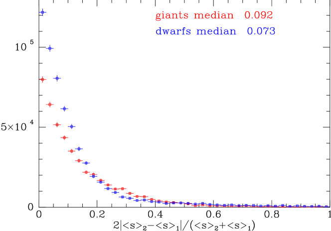
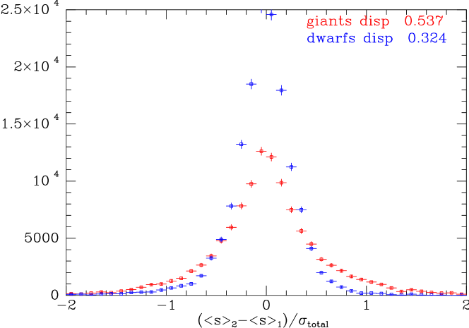
Figure 4: Top: the distribution of fractional differences in distances from repeat observations. Bottom: the distribution of distance differences divided by the quadrature-sum of the formal errors of each distance. As in Fig. 1, the quantity plotted vertically is the number of stars in each bin divided by the bin’s width, and the vertical bars show the statistical uncertainty.

Figure 5: The distribution for $15\,525$ stars with $3.3<\log g<3.7$ of the differences $s_{\rm VDR2}-s_{\rm VDR3}$ normalised by the quadrature sum of the formal errors.

4.4 Consistency of distances to subgiants

Our use of distinct pipelines to assign parameters to stars with $\log g<3.5$ and $\log g>3.5$ raises the question of whether distances are assigned consistently to stars that have $\log g\simeq 3.5$, which may lie on one side of the dividing line rather than the other merely by virtue of noise. Fig. 5 addresses this concern by comparing the VDR2 and VDR3 distances for the $15\,525$ stars with $\log g$ in $(3.3,3.7)$. It shows the distribution of $s_{\rm VDR2}-s_{\rm VDR3}$ normalised by the quadrature sum of the formal errors in each distance. The mean of the distribution is extremely small ($-9\times 10^{-5}$) although the mode of the distribution lies near $0.1$. It is to be expected that the higher values of $\log g$ returned by VDR3 should yield the smaller distances so we expect the peak in Fig. 5 to lie at a positive value of the ordinate. In view of the small value of the mean of the distribution, using one pipeline rather than the other for stars in the transition region cannot be said systematically to bias the derived distance.

4.5 Comparison with Zwitter et al. (2010)

It is interesting to compare our distances with those derived from the same spectra by Zwitter et al. (2010), which gives distances obtained from the VDR3 pipeline with three different isochrone sets. Here we consider only the distances Zwitter et al. obtained from Padova isochrones. We use the “new, revised” distances described in the note added to Zwitter et al. (2010) in proof; these distances use the less conservative error estimates to which the analysis of Siebert et al. (2011) gives rise. Our distances continue to be based on the older, more conservative error estimates of Zwitter et al. (2008).

The final column of Table 3 shows the distances Zwitter et al. find for the cluster stars. The formal errors on these distances are smaller than ours on account of the less conservative errors that Zwitter et al. adopted for the input parameters. Otherwise the agreement with our distances is excellent. In the case of OCL00148_1373319, for which the difference between our distance and the literature value is largest $(1.25\sigma)$, the Zwitter et al. distance lies closer to the literature value than our distance does, although it is still larger than expected by $1.5\sigma$. This star lies at Galactic latitude $b=3.6^{\circ}$, while most RAVE stars lie at much higher latitudes; only 5622 of the spectra under consideration come from $|b|<6^{\circ}$. The distances derived for OCL00148_1373319 from RAVE data may be too large because the star is significantly obscured and we have neglected obscuration.

The upper panel of Fig. 6 shows the distributions of the normalized residuals between our distances and those of Zwitter at al. when all stars are taken together. The mean normalised residual is pleasingly small, $0.02$. The lower panel shows the distribution of normalised residuals for giants and dwarfs taken separately. The dwarfs have quite a narrow distribution of residuals (dispersion 0.52) but they are offset from zero by 0.14, implying that the Zwitter et al. distances to dwarfs are systematically smaller than ours. We saw in §4.1 a tendency for our parallaxes for hot dwarfs to be larger than those measured by Hipparcos, so for these stars our distances are already too small. Thus the Zwitter et al. distances are offset from ours in the opposite direction from what one would expect if they were more accurate than ours. This result undoubtedly reflects the fact that all the Zwitter et al. distances are based on the VDR3 pipeline, which as Figure 2 attests, over-estimates $\log g$ for hot dwarfs.

At $0.52$ the dispersion of the normalised residuals of the dwarfs in Fig. 6 is substantially smaller than unity but larger than the dispersion of repeat observations of dwarfs (Fig. 4). This situation is what one would expect given that the Zwitter et al. distances and ours derive from the same data but processed with different versions of both the reduction pipeline and the algorithm used to extract distances from stellar parameters.

In Fig. 6 the distribution of normalised residuals between the Zwitter et al. distances for giants and ours is quite wide (dispersion $0.86$) and offset in the opposite direction to the distribution of dwarfs: the Zwitter et al. distances for giants tend to be larger than ours. Since the top right panel of Fig. 1 implies that our distances for giants are already larger than the Hipparcos parallaxes imply, the implication is that the Zwitter et al. distances for giants are less accurate than ours.

Whereas in Fig. 6 there is a contribution to the distribution of normalised residuals for dwarfs from the different pipelines used (VDR2 versus VDR3), there is no such contribution to the broader distribution of residuals for giants, and the entire width of the giant distribution derives from the different algorithms used to extract distances from a given set of stellar parameters.

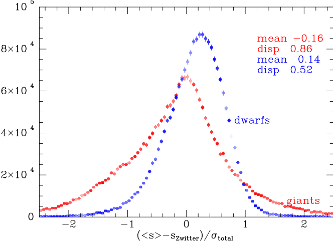
Figure 6: Comparison of our results with those of Zwitter et al. (2010). Top panel: all $215\,167$ stars with two distances; lower panel: stars with $\log g\geq 3.5$ or $<3.5$ grouped separately. The statistical uncertainties can be seen to be smaller than some of the points.

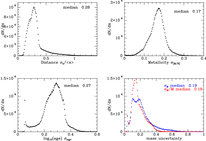
Figure 7: Distributions of output errors for all four stellar parameters: distance $s$ (top left); metallicity (top right); age (lower left); mass (lower right).

In fact the residual distribution can be understood in terms of of the different priors used here and in Zwitter et al.: whereas our prior recognises the existence of three components in the Galaxy, Zwitter et al. used a simple prior involving an IMF and a magnitude-dependent effect to represent the probability of a star entering a magnitude-limited sample under the assumption of constant volume density. First, our prior incorporates the spatial inhomogeneity of the Galaxy’s discs, which pulls stars towards smaller distances, particularly at high Galactic latitudes. The effect on dwarf stars can be expected to be rather small, but the effect on giants is more marked: in order to fall into the survey’s magnitude limits (which include both low- and high-magnitude cuts), a giant would have to be at a reasonable distance from the Sun, at which point (due to RAVE’s range of Galactic latitudes) the disc’s structure begins to play a significant role. This accounts for the leftwards wing of the red histogram in the bottom panel of Fig. 6.

Second, we also have a prior on stellar age that favours older ages. This prior increases the likely luminosity of a star of given initial mass over the most probable luminosity derived from the prior of Zwitter et al.. Consequently, we identify a significant number of stars as giants that Zwitter et al. considered to be dwarfs or subgiants. These stars appear as a noticeable positive wing in the red histogram of Fig. 6.

Aside from these substantial differences in approach, the different IMF and metallicity distributions taken in our study and that of Zwitter et al. make the small remaining spread seen in Fig. 6 eminently reasonable.

5 Output precisions

Fig. 7 shows the distribution of formal errors in each stellar parameter for the whole RAVE sample. Comparing these distributions with those in figs. 3 and 10 of Burnett & Binney (2010), we see that our precisions are noticeably higher than forecast. The median formal error in distance is 28%, and in §4.3 we saw that repeat observations suggested that the random errors are likely only half as large. The median input error in metallicity from the catalogue is $0.237$, while the top right panel of Fig. 7 shows that the median output error is $0.17$, so use of the prior diminishes the uncertainty by 29%. This reduction is consistent with the small scatter in Fig. 1 of Burnett & Binney (2010).

6 The selection function

Even though RAVE has one of the simplest and best-defined selection criteria of any large survey of the Galaxy, selection is based on colour and magnitude on the sky, and it is a non-trivial exercise to compute the resulting fraction of the stars in a given location in space that will be in the catalogue. Until these fractions are better determined, we cannot infer spatial densities of stars in the Galaxy from counts of stars in the RAVE catalogue. Hence at this stage we are restricted to three lines of enquiry: (i) what stars does the survey capture?, (ii) how do the distributions of stellar parameters vary with position in the Galaxy?, and (iii) how do the Galaxy’s kinematics vary with position, age and metallicity? In this section we focus on the first two lines of enquiry. Our distances and other parameters will be used elsewhere to study the Galaxy’s kinematics.

Figure 8: The distribution of derived absolute magnitudes in slices of Galactic latitude ($|b|$). The same vertical scale is used for all four panels so one gets an impression of the latitude-distribution of the entire sample.

Figure 9: The distribution of derived absolute magnitudes in ranges of Galactic longitude ($l$). The same vertical scale is used for all three panels so one gets an impression of the longitude-distribution of the entire sample.

In Fig. 8 we show the distribution of absolute $J$-magnitudes in different slices of Galactic latitude. The distributions are strongly bimodal: the red clump produces a narrow peak at $\langle M_{J}\rangle\sim-1$ and turnoff stars a broader peak around $\langle M_{J}\rangle\sim 3$. At $|b|<25^{\circ}$ clump stars completely dominate, while the turnoff stars outnumber giants above $|b|\sim 40^{\circ}$. This progression reflects the steepening gradient in the density of stars along the line of sight with increasing $|b|$ since clump stars must have a distance modulus of more than 8, and a distance $\ga 400\,\rm{pc}$, to enter the survey, and towards the pole there are many fewer stars at such distances than nearby dwarfs. In the absence of a steep gradient along the line of sight, clump stars dominate the survey because the latter was designed to select disc giants. Moreover the fraction of giants at $|b|<25^{\circ}$ is enhanced by the fact that during most of the survey a colour cut $J-K>0.5$ has been imposed in the region $230^{\circ}<l<315^{\circ}$, $|b|<25^{\circ}$ precisely in order to favour the selection of giants – elsewhere selection has been on magnitude alone.

Fig. 9 shows how the distribution in absolute magnitude varies with Galactic longitude. As the argument just given leads one to expect, giants are less prominent towards the anticentre than towards either the inner Galaxy or the tangent directions. However, the distributions in $l$ are strongly influenced by the survey’s non-uniform sky coverage. Towards the Galactic centre, the RAVE fields extend much closer to the Galactic plane, and in such fields giants will be particularly prominent.

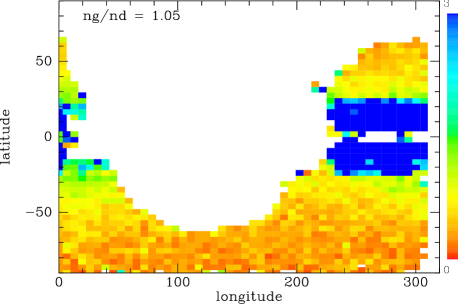
Figure 10: The variation across the sky of the giant/dwarf fraction, with giants defined by $\langle M_{J}\rangle<1$ and dwarfs by $\langle M_{J}\rangle\geqslant 1$. White regions are not sampled by RAVE.

It is interesting to compare the variation over the sky of the giant/dwarf ratio with that predicted by the Galaxy modelling code Galaxia (Sharma et al., 2011) for a survey with RAVE’s selection function. Fig. 10 shows the observed giant/dwarf ratio, while the bottom panel of Fig. 11 shows the prediction of Galaxia for this figure. The top two panels of Fig. 11 show that the predictions of Galaxia depend significantly on the model of extinction by dust (which is that of Bland-Hawthorn et al. 2010) by showing the giant/dwarf ratio predicted with (middle panel) and without (top panel) including extinction. The middle and bottom panels of Fig. 11 show the impact on the predicted giant/dwarf ratio of RAVE’s handling of low-latitude regions, especially the imposition of the colour condition $J-K>0.5$ at $225^{\circ}<l<315^{\circ}$. In both Fig. 10 and the bottom panel of Fig. 11 the giant/dwarf ratio is above unity only within $\sim 25^{\circ}$ of the plane, but near the plane it achieves very large values – in Fig. 10 there are cells with more than 10 dwarfs and $n_{\rm g}/n_{\rm d}>54$ – both on account of the length of sight lines through the disc, and on the imposition of the colour cut $J-K>0.5$, which enhances the giant fraction. Consequently, the dark blue region of Fig.10 is heavily saturated. The numbers in the top left corner of each panel give the ratio $n_{\rm g}/n_{\rm d}$ of the total number of giants to dwarfs, which is $1.05$ for the data and $1.39$ for the model. Given residual uncertainty as to what RAVE’s selection function is at low latitudes, we consider the agreement between the values of $n_{\rm g}/n_{\rm d}$ from the data and Galaxia to be satisfactory.

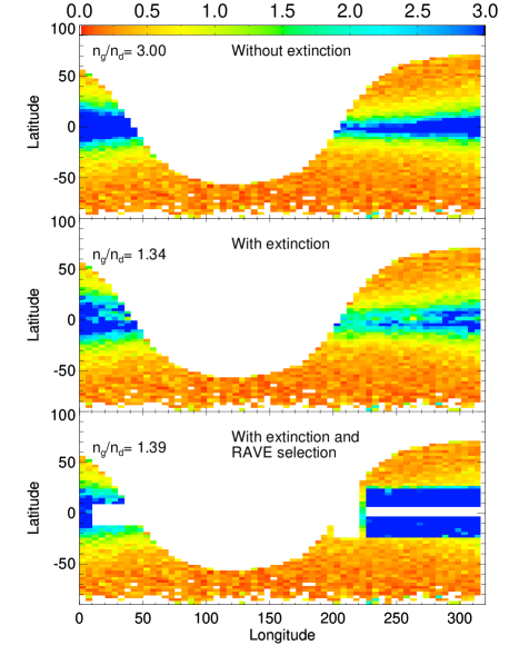
Figure 11: The prediction of the Galaxy modelling code Galaxia (Sharma et al., 2011) for the structure of Fig. 10. The top two panels show all stars with $9<I<12$, without (top) and with (middle) including Galactic extinction. In the bottom panel low-latitude fields have been excluded and for $<225^{\circ}<l<315^{\circ}$ only stars with $J-K>0.5$ are included.

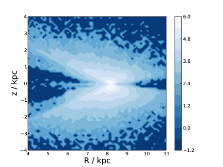
Figure 12: The distribution of observed stars in the $(R,z)$ plane. Contours are logarithmically spaced and represent densities in $\log\!\left({\rm stars\;kpc}^{-2}\right)$.

7 Parameter distributions

What does RAVE tell us about the variation from point to point in the Galaxy in the distribution of stars over age and metallicity? We must bear in mind that our prior has a bigger impact on these stellar parameters than on distances. Consequently, we investigate the effect of our prior on the results.

7.1 Region probed by survey

Fig. 12 shows the density of observed stars in the $(R,z)$ plane. The density seen here is the product of three factors: (i) the intrinsic density of stars in the Galaxy, (ii) variation with distance from the Sun that follows from the survey’s faint and bright magnitude limits and the stellar luminosity function, and (iii) a bias against objects in the plane that is driven by a combination of obscuration and the survey’s avoidance of low-latitude fields. Notwithstanding the strong impact of the biases (ii) and (iii), the basic structure of the Galactic disc is evident in Fig. 12.

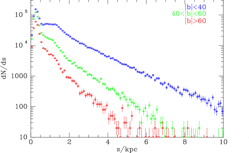
Figure 13: Histograms of the distribution in distance of RAVE stars in three ranges of Galactic latitude.

Regardless of the extent to which the density of observed stars reflects the Galaxy’s intrinsic structure or selection effects, it tells us for which regions the survey carries useful information. At the solar radius this extends to $\sim 3\,\rm{kpc}$ above and below the plane, and beyond the solar circle there is a steady but gradual narrowing in the width in $z$ of the surveyed region with increasing $R$. Towards the centre the surveyed region terminates at larger values of $|z|$ than towards the anticentre. Fig. 13 shows the distribution in distance of stars in three ranges of Galactic latitude: $|b|<40^{\circ}$, $40^{\circ}\leq|b|<60^{\circ}$ and $|b|\geq 60^{\circ}$. The median distances in these three classes are $1.03\,\rm{kpc}$ for $|b|<40^{\circ}$, $450\,\rm{pc}$ for $40^{\circ}\leq|b|<60^{\circ}$ and $372\,\rm{pc}$ for $|b|\geq 60^{\circ}$.

7.2 Metallicity

We now look at the variation of mean metallicity with distance from the Galactic plane. We have two different sets of metallicities to work with, since each star has both an observed value and that returned by the model fitting. We plot both sets of data simultaneously in Fig. 14. Since the model isochrones only cover metallicities down to $\hbox{[M/H]}=-0.914$, distributions of output metallicities for $|z|\geq 1\,\rm{kpc}$ show a tendency for stars to pile up near this limit. At lower heights the output distributions are distinctly tighter than those observed, and below $\sim 300\,\rm{pc}$ they are displaced to slightly lower [M/H]. The output histograms tend to negligible values well ahead of the metallicity of the most metal-rich isochrone ($\hbox{[M/H]}=0.54$), suggesting that there really are extremely few stars with $\hbox{[M/H]}_{\rm t}>0.2$. The median value of the observational error for each slice (estimated via eq. 3 in this paper and eq. 22 of Zwitter et al. 2008) is shown as a red scale bar on each panel, and, given that there are smaller errors on our output metallicities, it can be seen that, apart from the bias to low metallicity just discussed, the scale of these errors is very reasonable to explain the difference between the blue and red distributions in each case.

The progression that would be expected in metallicity is clearly visible as one moves away from the plane: from a narrow thin-disc distribution at low $|z|$, there is a gradual shift to a broader thick-disc distribution beyond around one thin-disc scale height, $\sim 0.3\,\rm{kpc}$, moving towards a significantly lower-metallicity halo distribution as one moves beyond the thick disc scale height, 0.9 kpc. Unfortunately, the isochrones we have used are all too metal-rich for halo stars, so in Fig. 14 the small number of halo stars in the RAVE sample cause an un-physical peak in the blue points at $\hbox{[M/H]}=-0.9$. The metallicity distribution for $1\,\rm{kpc}<|z|<1.8\,\rm{kpc}$ is similar to that found by Bensby et al. (2007) for thick-disc stars except that ours extends $\sim 0.1\,$dex less far on the metal-poor side.

From SDSS data Ivezić et al. (2008) concluded that the median metallicity in the disc decreases from $\hbox{[M/H]}_{\rm t}=-0.6$ at $|z|=500\,\rm{pc}$ to $-0.8$ beyond several kiloparsecs. Fig. 14 implies that at $|z|=500\,\rm{pc}$ the median disc metallicity is $>-0.1$, and even at $|z|>2\,\rm{kpc}$ it is no smaller than $-0.5$.

Close to the plane the natural comparison is with the metallicity distribution within the Geneva-Copenhagen survey (GCS) of Hipparcos stars (Nordström et al., 2004; Holmberg et al., 2009). Unfortunately, the metallicities of these stars are somewhat controversial. Fuhrmann (2008) finds that high-resolution spectroscopy of a sample of only 185 local F and K stars implies that the solar-neighbourhood distribution in [Mg/H] covers $(-0.2,0.2)$, while Haywood (2006) argues that the metallicity distribution of young stars is intrinsically narrow and the spread in measured values of $\sim 0.1\,$dex is dominated by measurement error. The bottom panel of Fig. 14 suggests that near the plane, the intrinsic spread in the metallicity is indeed narrow.

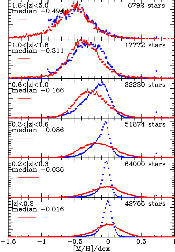
Figure 14: The distribution in metallicity at several distance from the Galactic plane. Red points show observed metallicities, blue points show the output from our analysis. Values of $|z|$ are in kpc, and the median output metallicity for each slice is displayed. The red scale bar in each panel represents the median observational error for that subsample.

The means of the distributions of input and output metallicities shown in Fig. 14 lie close to one another at all values of $|z|$. Fig. 15 makes this fact clear by showing the output distribution in blue superimposed on the wider input distribution, plotted in red. The similarities of these means implies that the blue output metallicities are not merely reproducing our prior.

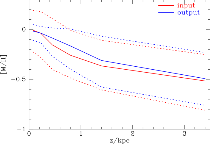
Figure 15: The variation in the metallicity distribution as one moves away from the plane. Red: observed metallicities, blue: output metallicities. The solid line represents the median of each distribution and dashed lines show $1\sigma$ variations from the median.

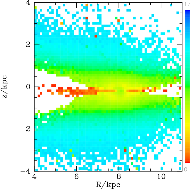
Figure 16: The distribution of average stellar age in the $(R,z)$ plane. The colour scale gives ages in Gyr. Regions for which there is inadequate data are white.

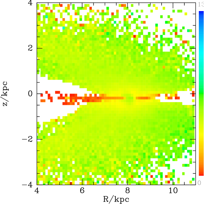
Figure 17: As Fig. 16, but when the data are analysed with a prior that is completely flat in age.

7.3 Stellar ages

Stellar ages are extremely hard to determine reliably. The most reliable ages are those obtained from the location in the $(T_{\rm eff},L)$ of slightly evolved main-sequence stars with independently determined distances. Since we do not know the distances to stars a priori, our ages must be suspect. They are nonetheless of interest as sanity checks on the performance of the algorithm. They may even be serve as indicators of possible trends in the data, since even in the absence of an independent distance estimate for a star, the spectrum combined with the star’s photometry does provide some indication of its age.

Fig. 16 displays a colour-scale plot of the average stellar age across the $(R,z)$ plane. To some extent this distribution reflects our prior, but it is encouraging to see that the map conforms to our intuition: at small $|z|$ a young disc is dominant. This young structure dwindles as one moves outwards in $R$ and away from $z=0$. Far from the plane, the gradient in age becomes small, consistent with these regions being dominated by an old population that is not strongly concentrated to the plane.

Note that shapes of the contours in Fig. 12 and Fig. 16 are quite different. This fact is reassuring, for it tells us that the measured age distribution remains stable even when the survey picks up only a small fraction of the Galaxy’s stars.

Fig. 17 addresses the fear that the age gradient evident in Fig. 16 is an artifact produced by our chosen prior, by showing the distribution one obtains with a prior that is completely flat in age from the present back to age 13.7 Gyr; all other elements of the prior (metallicity, number density, IMF) were unchanged. We see that dropping the prior causes the mean age for many regions to become $\sim 6\,\rm{Gyr}$. This happens because with a flat age prior, the age pdfs of stars become broad and their means shift towards the centre of the permitted range. Although age is less strongly correlated with $|z|$ in Fig. 17 than in Fig. 16, the youngest stars remain concentrated to the plane, and above the plane there is a tendency for mean age to increase with $R$ at fixed $z$ as we expect if a tapering young disc is superimposed on a broader old population of thick-disc and halo stars. Thus although the prior is having a significant effect on the age distribution we recover from RAVE, it is not entirely responsible for the nice age distribution seen in Fig. 16.

In Fig. 16 the immediate vicinity of the Sun seems to have a slightly older population than points just above the plane and $\sim 1\,\rm{kpc}$ further in or out. The number of stars seen near the plane and $\sim 1\,\rm{kpc}$ from the Sun is small (Fig. 12) and the stars we do see have a high probability of being obscured by dust. The obscuration will select against low-luminosity stars and thus favour the entry into the catalogue of hot young stars. It will also affect age determinations, but in an unpredictable way because $T_{\rm eff}$ will be changed as well as the broad-band colours. Moreover, in low-latitude fields unusual objects were deliberately targeted by the RAVE survey. Consequently, the data for low-latitude regions that lie $\sim 1\,\rm{kpc}$ from the Sun are suspect, and the more gradual falloff in age with height near the Sun is likely to be more representative of the disc than the steeper gradient seen further away. A countervailing consideration is that the bright-magnitude limit of RAVE will exclude nearby young stars and thus bias the nearby data towards older stars. Reassuringly, when Galaxia is used to simulate Fig. 16, a similar distribution of ages is produced. In particular, within the plane the mean age of stars decreases with distance from the Sun for $s\la 1\,\rm{kpc}$.

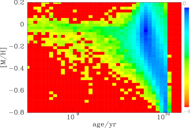
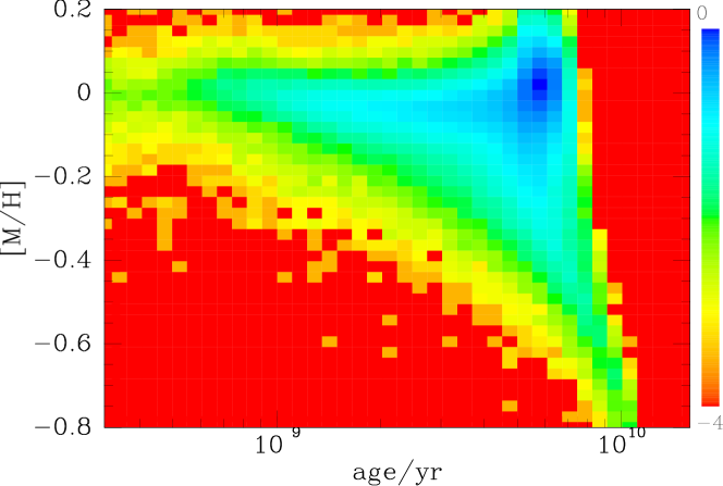
Figure 18: The distribution of stars in the age–metallicity plane at $|z|>500\,\rm{pc}$ (above) and $|z|<500\,\rm{pc}$ (below). The colour encodes the base-10 logarithm of stellar density, with red indicating a complete absence of stars. The values of [M/H] used are the outputs of the distance-finding algorithm.

7.4 Age-metallicity relation

Fig. 18 shows the distribution of stars in the age–metallicity plane at $|z|>500\,\rm{pc}$ in the upper panel and $|z|<500\,\rm{pc}$ in the lower panel. At high $|z|$ we see the expected concentration of thick-disc stars to high ages with a broad metallicity distribution. The ridge line of the population clearly shows a rapid increase in metallicity with time, to solar metallicity at an age of $6\,\rm{Gyr}$. Nearer the plane, there is a significant population of young stars and a lower envelope to the distribution that allows for relatively young stars that have distinctly sub-solar metallicities. The highest density of thin-disc stars occurs at $\hbox{[M/H]}_{\rm t}\simeq 0$ and age $\sim 6\,\rm{Gyr}$, distinctly younger than the maximum permitted age of disc stars. And at $\hbox{[M/H]}_{\rm t}\simeq 0$ the density of stars tails off rapidly at ages in excess of $6\,\rm{Gyr}$. At earlier times only metal-poor stars formed, and the rate at which they did so appears to have been flat or even increasing with time, while at later times the star-formation rate must have declined steadily with time.

While these trends are interesting and consistent with a plausible scenario for the chemical evolution of the Galaxy, they should not be assigned much weight for the reasons given at the start of §7.3. It is also worth noting that the plots in Fig. 18 differ in important respects from equivalent plots produced by Galaxia. In particular, the synthetic plots for $|Z|>500\,\rm{pc}$ do not show a region of high density at $(\tau=6\,\rm{Gyr},\hbox{[M/H]}_{\rm t}>0)$, and, with the expected errors in $\log\tau$, the distribution of ages at $\hbox{[M/H]}<-0.4$ is significantly wider than in Fig. 18.

8 Conclusions

We have derived distances (or parallaxes) to $\sim 216\,000$ stars in the RAVE survey using the Bayesian analysis of Burnett & Binney (2010). We have checked the parallaxes and their associated errors against Hipparcos parallaxes, and conclude that for dwarfs cooler than $T_{\rm eff}=6000\,{\rm K}$ the parallaxes are unbiased, but the parallaxes of hotter dwarfs are systematically too large by $\sim 0.1\sigma$ because even the VDR2 pipeline over-estimates the gravities of hot dwarfs. The parallaxes of giants tend to be too small by $\sim 0.1\sigma$. For all three classes of star, hot dwarfs, cool dwarfs and giants, the scatter in differences between the spectrophotometric and Hipparcos parallaxes is consistent with the formal errors on the parallaxes.

We have checked our distances and our errors against distances to star clusters, which tend to be beyond the reach of Hipparcos. This rather small sample of stars, which contains both dwarfs and giants, is consistent with our distances being unbiased and their errors being accurate.

RAVE has obtained more than one spectrum for $\sim 19\,000$ stars. We have used this sample to assess our errors by comparing independent distances to the same object. The scatter in the difference of distances is only half the quadrature-sum of their formal errors. This is consistent with a significant contribution to the errors coming from factors, such as defects in the spectral analysis and the physics of the stellar models, that are the same for repeated determinations of the distance to a given star.

Comparison of our distances to the spectrophotometric distances of Zwitter et al. (2010) shows that we assign slightly larger distances to dwarfs and smaller distances to giants than do Zwitter et al. Given the signs of our deviations from Hipparcos parallaxes, it follows that for both dwarfs and giants our distances are more accurate than those of Zwitter et al. For dwarfs this finding can be traced to the use by Zwitter et al. of the VDR3 pipeline, which tends to over-estimate $\log g$, especially for hot dwarfs. Our distances to giants benefit from a more sophisticated prior, which tends to pull stars to smaller distances. For dwarfs the distribution of normalised residuals between our distances and those of Zwitter et al. is rather narrow, having a dispersion of only $0.52$, implying that much of the uncertainty in distance arises from errors in the original data and the spectral template library, which are common to the two studies.

Our formal errors are based on the conservative estimates of the errors in the input data given by Zwitter et al. (2008). The conservative nature of these errors is confirmed by the analyses of both repeat observations and the distances of Zwitter et al. (2010). However, the analysis of Hipparcos stars indicates that by happy chance our formal error budget is just large enough to encompass external sources of error, such as spectral mis-match and deficiencies in the stellar models, so our formal errors are close to the final uncertainties in our distances.

We have examined the distributions of the errors returned by the Bayesian analysis for distance, metallicity, age and initial mass. The median formal distance error is $28\%$, the median formal uncertainty in [M/H] is 0.17 dex, the median formal uncertainty in $\log(\tau)$ is 0.27 dex and the median fractional uncertainty in initial mass is $16\%$. These figures show that by using prior knowledge of the structure of our Galaxy and the nature of stellar evolution, one can constrain stellar parameters more narrowly than when each spectrum is considered in isolation.

Data gathered during the pilot part of the RAVE survey has now been released (Siebert et al., 2011), and the distances we derive from these data are contained in the release. In view of our results for the Hipparcos stars, it may be useful to correct the distances of dwarfs with $T>6000\,$K by increasing their distances by 10% of their formal errors, and to correct the distances of giants by decreasing their distances by the same amount.

Our distances reveal which parts of the Galaxy the RAVE survey probes. Roughly half the stars in the RAVE catalogue are giants and half dwarfs. The giant/dwarf ratio varies strongly with Galactic latitude and to a weaker extent with Galactic longitude. The structure of the variation is accurately predicted by Galaxia when obscuration by dust is included, which significantly reduces the fraction of giants seen towards the Galactic Centre. Although the spatial distribution of RAVE stars reflects the survey’s selection function as well as the intrinsic stellar density of the Galaxy, it nonetheless reveals the double-exponential structure of the disc. Moreover, the distribution of stellar ages shows the expected concentration of young stars towards the plane.

The metallicity distribution evolves systematically with distance from the plane, being remarkably narrow and slightly sub-solar at $|z|<150\,\rm{pc}$, to much broader and centred on $\hbox{[M/H]}\simeq-0.5$ more than $2\,\rm{kpc}$ up. Our results support the view that observational errors have the biggest impact on the observed metallicity distribution near the plane.

This work has brought into sharp focus the crucial importance of the pipeline that extracts stellar parameters from the raw spectra. A valuable upgrade to the current pipeline would be to force the parameters assigned to a star to be consistent with models of stellar evolution. This upgrade, which is mandatory from the perspective of Bayesian inference, would eliminate the high density of stars in the bottom-right panel of Fig. 2 at $\log g\simeq 5$ and $T_{\rm eff}>6000\,{\rm K}$. This study also highlights the need for a more sophisticated analysis of the errors in the parameters returned by the pipeline. For example, one would expect the error on $\log g$ to depend on [M/H] in addition to S/N, which we have had to assume has complete control of the errors in the input parameters. Moreover, near the turnoff the errors in $T_{\rm eff}$ and $\log g$ will be quite strongly correlated, and we have had to neglect this fact. All improvements in the pipeline will feed through into more accurate distances.

The distances and stellar parameters described here provide a basis for extensive work on the structure, kinematics and dynamics of our Galaxy. Work on the Galaxy’s kinematics is already underway, and papers in this area will appear shortly. Work on the Galaxy’s dynamics requires characterisation of the intrinsic density distribution of the population(s) whose kinematics have been measured. Determining those densities involves determination of the survey’s selection function. This is the next major task that must be accomplished before the RAVE survey can attain its ultimate goals.

References

- Aumer & Binney (2009) Aumer, M. & Binney, J. J. 2009, MNRAS, 397, 1286
- Bensby et al. (2007) Bensby, T., Zenn, A. R., Oey, M. S., & Feltzing, S. 2007, ApJ, 663, L13
- Bertelli et al. (2008) Bertelli, G., Girardi, L., Marigo, P., & Nasi, E. 2008, A&A, 484, 815
- Bland-Hawthorn et al. (2010) Bland-Hawthorn, J., Krumholz, M. R., & Freeman, K. 2010, ApJ, 713, 166
- Breddels et al. (2010) Breddels, M. A., Smith, M. C., Helmi, A., et al. 2010, A&A, 511, A90+
- Burnett & Binney (2010) Burnett, B. & Binney, J. 2010, MNRAS, 407, 339
- Fuhrmann (2008) Fuhrmann, K. 2008, MNRAS, 384, 173
- Haywood (2006) Haywood, M. 2006, MNRAS, 371, 1760
- Holmberg et al. (2009) Holmberg, J., Nordström, B., & Andersen, J. 2009, A&A, 501, 941
- Ivezić et al. (2008) Ivezić, Ž., Sesar, B., Jurić, M., et al. 2008, ApJ, 684, 287
- Ivezić et al. (2001) Ivezić, Ž., Tabachnik, S., Rafikov, R., et al. 2001, AJ, 122, 2749
- Jørgensen & Lindegren (2005) Jørgensen, B. R. & Lindegren, L. 2005, A&A, 436, 127
- Kroupa et al. (1993) Kroupa, P., Tout, C. A., & Gilmore, G. 1993, MNRAS, 262, 545
- Munari et al. (2009) Munari, U., Siviero, A., Bienaymé, O., et al. 2009, A&A, 503, 511
- Nordström et al. (2004) Nordström, B., Mayor, M., Andersen, J., et al. 2004, A&A, 418, 989
- Perryman (1997) Perryman, M. 1997, The Hipparcos and Tycho Catalogues (Noordwijk: ESA Publications)
- Pont & Eyer (2004) Pont, F. & Eyer, L. 2004, MNRAS, 351, 487
- Seabroke et al. (2008) Seabroke, G. M., Gilmore, G., Siebert, A., et al. 2008, MNRAS, 384, 11
- Sharma et al. (2011) Sharma, S., Bland-Hawthorn, J., Johnson, K., & Binney, J. 2011, ApJ, 730, in press
- Siebert et al. (2008) Siebert, A., Bienaymé, O., Binney, J., et al. 2008, MNRAS, 391, 793
- Siebert et al. (2010) Siebert, A., Famaey, B., Minchev, I., Seabroke, G. M., & RAVE collaboration. 2010, MNRAS, submitted
- Siebert et al. (2011) Siebert, A., Williams, M., Siviero, A., et al. 2011, AJ, xxx
- Skrutskie et al. (2006) Skrutskie, M. F., Cutri, R. M., Stiening, R., et al. 2006, AJ, 131, 1163
- Smith et al. (2007) Smith, M. C., Ruchti, G. R., Helmi, A., et al. 2007, MNRAS, 379, 755
- Steinmetz et al. (2006) Steinmetz, M., Zwitter, T., Siebert, A., et al. 2006, AJ, 132, 1645
- Tsvetkov et al. (2008) Tsvetkov, A. S., Popov, A. V., & Smirnov, A. A. 2008, Astronomy Letters, 34, 17
- van Leeuwen (2007) van Leeuwen, F., ed. 2007, Astrophysics and Space Science Library, Vol. 350, Hipparcos, the New Reduction of the Raw Data
- York et al. (2000) York, D. G., Adelman, J., Anderson, Jr., J. E., et al. 2000, AJ, 120, 1579
- Zwitter et al. (2010) Zwitter, T., Matijevič, G., & et al., M. A. B. 2010, A&A, 522, 54
- Zwitter et al. (2008) Zwitter, T., Siebert, A., Munari, U., et al. 2008, AJ, 136, 421