Terapixel imaging of cosmological simulations

Abstract

The increasing size of cosmological simulations has led to the need for new visualization techniques. We focus on Smoothed Particle Hydrodynamical (SPH) simulations run with the GADGET code and describe methods for visually accessing the entire simulation at full resolution. The simulation snapshots are rastered and processed on supercomputers into images that are ready to be accessed through a web interface (GigaPan). This allows any scientist with a web-browser to interactively explore simulation datasets in both in spatial and temporal dimensions, datasets which in their native format can be hundreds of terabytes in size or more. We present two examples, the first a static terapixel image of the MassiveBlack simulation, a P-GADGET SPH simulation with 65 billion particles, and the second an interactively zoomable animation of a different simulation with more than one thousand frames, each a gigapixel in size. Both are available for public access through the GigaPan web interface. We also make our imaging software publicly available.

1. Introduction

In the 40 years that $N$-body simulations have been used in Cosmology research, visualization has been the most indispensable tool. Physical processes have often been identified first and studied via images of simulations. A few examples are: formation of filamentary structures in the large-scale distribution of matter (Jenkins et al., 1998; Colberg et al., 2005; Springel et al., 2005; Dolag et al., 2006), growth of feedback bubbles around quasars (Sijacki et al., 2007; Di Matteo et al., 2005); cold flows of gas forming galaxies (Dekel et al., 2009; Keres et al., 2005), and the evolution of ionization fronts during the re-ionization epoch (Shin et al., 2008; Zahn et al., 2007). The size of current and upcoming Peta-scale simulation datasets can make such visual exploration to discover new physics technically challenging. Here we present techniques that can be used to display images at full resolution of datasets of hundreds of billions of particles in size.

Several implementations of visualization software for cosmological simulations already exist. IRFIT (Gnedin, 2011) is a general purpose visualization suite that can deal with mesh based scalar, vector and tensor data, as well as particle based datasets as points. YT (Turk et al., 2011) is an analysis toolkit for mesh based simulations that also supports imaging. SPLASH (Price, 2007) is a visualization suite specialized for simulations that use smoothed particle hydrodynamics(SPH) techniques. Aside from the CPU based approaches mentioned above, Szalay et al. (2008) implemented a GPU based interactive visualization tool for SPH simulations.

The Millennium I & II simulations (Springel et al., 2005; Boylan-Kolchin et al., 2009) have been used to test an interactive scalable rendering system developed by Fraedrich et al. (2009). Both SPLASH and the Millennium visualizer support high quality visualization of SPH data sets, while IRFIT treats SPH data as discrete points.

Continuing improvements in computing technology and algorithms are allowing SPH cosmological simulations to be run with ever increasing numbers of particles. Runs are now possible on scales which allow rare objects, such as quasars to form in a large simulation volume with uniform high resolution (see Section 2.1; and Di Matteo et al. (2011, in prep); Degraf et al. (2011, in prep); Khandai et al. (2011, in prep)). Being able to scan through a vast volume and seek out the tiny regions of space where most of the activity is occurring, while still keeping the large-scale structure in context necessitates special visualization capabilities. These should be able to show the largest scale information but at the same be interactively zoomable. However, as the size of the datasets quickly exceeds the capability of moderately sized in-house computer clusters, it becomes difficult to perform any interactive visualizations. For example, a single snapshot of the MassiveBlack simulation (Section 2.1) consists of 8192 files and is over 3 TB in size.

Even when a required large scale high resolution image has been rendered, actually exploring the data requires special tools. The GigaPan collaboration has essentially solved this problem in the context of viewing large images, with the GigaPan viewer enabling anyone connected to the Internet to zoom into and explore in real time images which would take hours to transfer in totality. The viewing technology has been primarily used to access large photographic panoramas, but is easily applicable to simulated datasets. A recent enhancement to deal with the time dimension, in the form of gigapixel frame interactive movies (GigaPan Time Machine) will turn out to give particularly novel and exciting results when applied to simulation visualization.

In this work we combine an off-line imaging technique together with GigaPan technology to implement an interactively accessible visual probe of large cosmological simulations. While GigaPan is an independent project (uploading and access to the GigaPan website is publicly available), we release our toolkit for the off-line visualization as Gaepsi, a software package aimed specifically at GADGET (Springel et al., 2001; Springel, 2005) SPH simulations.

The layout of our paper is as follows. In Section 2 we give a brief overview of the physical processes modeled in GADGET, as well as describing two P-GADGET simulations which we have visualized. In Section 3 we give details of the spatial domain remapping we employ to convert cubical simulation volumes into image slices. In Section 4, we describe the process of rasterizing an SPH density field, and in Section 5 the image rendering and layer compositing. In Section 6 we address the parallelism of our techniques and give measures of performance. In Section 7 we briefly describe the GigaPan and GigaPan Time Machine viewers and present examples screenshots from two visualizations (which are both accessible on the GigaPan websites).

2. Simulation

Adaptive Mesh Refinement(AMR, e.g., Bryan & Norman (1997)) and Smoothed Particle Hydrodynamics (SPH, Monaghan (1992)) are the two most used schemes for carrying out cosmological simulations. In this work we focus on the visualization of the baryonic matter in SPH simulations run with P-GADGET (Springel, 2005).

GADGET is an SPH implementation, and P-GADGET is a version which has been developed specifically for petascale computing resources. It simultaneously follows the self-gravitation of a collision-less N-body system (dark matter) and gas dynamics (baryonic matter), as well as the formation of stars and super-massive black holes. Dark matter particles and gas particle positions and initial characteristics are set up in a comoving cube, and black hole and star particles are created according to sub-grid modeling (Hernquist & Springel, 2003; Di Matteo et al., 2008) Gas particles carry hydrodynamical properties, such as temperature, star formation rate, and neutral fraction.

Although our attention in this paper is limited to imaging properties the of gas, stars and black holes in GADGET simulations, similar techniques could be used to visualize the dark matter content. Also, the software we provide should be easily adaptable to the data formats of other SPH codes (e.g. GASOLINE, (Wadsley et al., 2004))

2.1. MassiveBlack

The MassiveBlack simulation is the state-of-art SPH simulation of a $\mathsf{\Lambda CDM}$ universe (Di Matteo et al., 2011, in prep). P-GADGET was used to evolve $2\times 3200^{3}$ particles in a volume of side length $533\,\mathrm{h^{-1}Mpc}$ with a gravitational force resolution of $5\,\mathrm{h^{-1}Kpc}$. One snapshot of the simulation occupies 3 tera-bytes of disk space, and the simulation has been run so far to redshift $z=4.75$, creating a dataset of order $120$ TB. The fine resolution and large volume of the simulation permits one to usefully create extremely large images. The simulation was run on the high performance computing facility, Kraken, at the National Institute for Computational Sciences in full capability mode with 98,000 CPUs.

2.2. E5

To make a smooth animation of the evolution of the universe typically requires hundreds frames directly taken as snapshots of the simulation. The scale of the MassiveBlack run is too large for this purpose, so we ran a much smaller simulation (E5) with $2\times 336^{3}$ particles in a $50\,\mathrm{h^{-1}Mpc}$ comoving box. The model was again a $\mathsf{\Lambda CDM}$ cosmology, and one snapshot was output per 10 million years, resulting in 1367 snapshots. This simulation ran on $256$ cores of the Warp cluster in the McWilliams Center for Cosmology at CMU.

3. Spatial Domain Remapping

Spatial domain remapping can be used to transform the periodic cubic domain of a cosmological simulation to a patch whose shape is similar to the domain of a sky survey, while making sure that the local structures in the simulation are preserved (Carlson & White, 2010; Hilbert et al., 2009). Another application is making a thin slice that includes the entire volume of the simulation. Our example will focus on the latter case.

A GADGET cosmological simulation is usually defined in the periodic domain of a cube. As a result, if we let $f(X=(x,y,z))$ be any position dependent property of the simulation, then

$$f(X)=f((x+\mu L,y+\nu L,z+\sigma L)),$$

where $\mu,\nu,\sigma$ are integers. The structure corresponds to a simple cubic lattice with lattice constant $a=L$, the simulation box side-length. A bijective mapping from the cubic unit cell to a remapped domain corresponds to a choice of the primitive cell. Figure 1 illustrates the situation in 2 dimensions.

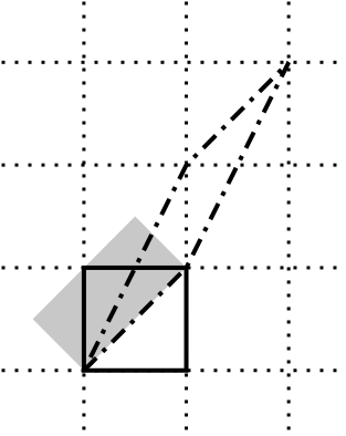
Figure 1.— Transformation of the Primitive Cell. The cubical unit cell is shown using solid lines. The new primitive cell, generated by $\left[\begin{smallmatrix}1&1\\ 1&2\end{smallmatrix}\right]$ is shown with dash-dotted lines. The transformed domain is shown in gray.

Whilst the original remapping algorithm by Carlson & White (2010) results in the correct transformations being applied, it has two drawbacks: (i) the orthogonalization is invoked explicitly and (ii) the hit-testing for calculation of the shifting (see below) is against non-aligned cuboids. The second problem especially undermines the performance of the program. In this work we present a faster algorithm based on similar ideas, but which features a QR decomposition (which is widely available as a library routine), and hit-testing against an AABB (Axis Aligned Bounding Box).

First, the transformation of the primitive cell is given by a uni-modular integer matrix,

$$M=\left(\begin{matrix}M_{11}&M_{12}&M_{13}\\ M_{21}&M_{22}&M_{23}\\ M_{31}&M_{32}&M_{33}\end{matrix}\right),$$

where $M_{ij}$ are integers and the determinant of the matrix $|M|=1$. It is straight-forward to obtain such matrices via enumeration. (Carlson & White, 2010) The $QR$ decomposition of $M$ is

$$M=QR,$$

where $Q$ is an orthonormal matrix and $R$ is an upper-right triangular matrix. It is immediately apparent that (i) application of $Q$ yields rotation of the basis from the simulation domain to the transformed domain, the column vectors in matrix $Q^{T}$ being the lattice vectors in the transformed domain; (ii) the diagonal elements of $R$ are the dimensions of the remapped domain. For imaging it is desired that the thickness along the line of sight is significantly shorter than the extension in the other dimensions, thus we require $0<R_{33}\ll|R_{22}|<|R_{11}|$. Note that if a domain that is much longer in the line of sight direction is desired, for example to calculate long range correlations or to make a sky map of a whole simulation in projection, the choice should be $0<|R_{33}|<|R_{22}|\ll|R_{11}|$.

Next, for each sample position $X$, we solve the indefinite equation of integer cell number triads $I=(I_{1},I_{2},I_{3})^{T}$,

$$\tilde{X} =Q^{T}X+aQ^{T}I,$$

where $a$ is the box size, $\tilde{X}$ is the transformed sample position satisfying $\tilde{X}\in[0,R_{11})\times[0,R_{22})\times[0,R_{33})$. In practice, the domain of $\tilde{X}$ is enlarged by a small number $\epsilon$ to address numerical errors. Multiplying by $Q$ on the left and re-organizing the terms, we find

$$I=\frac{Q\tilde{X}}{a}-\frac{X}{a}.$$

Notice that $Q\tilde{X}$ is the transformed sample position expressed in the original coordinate system, and is bounded by its AABB box. If we let $(Q\tilde{X}/a)_{i}\in[B_{i},T_{i}]$, where $B_{i}$ and $T_{i}$ are integers, and notice $\frac{X_{i}}{a}\in[0,1)$, the resulting bounds of $I$ are given by

$$I_{i}\in[B_{i},T_{i}].$$

We then enumerate the range to find $\tilde{X}$.

When the remapping method is applied to the SPH particle positions, the transformations of the particles that are close to the edges give inexact results. The situation is similar to the boundary error in the original domain when the periodic boundary condition is not properly considered. Figure 2 illustrates the situation by showing all images of the particles that contribute to the imaging domain. We note that for the purpose of imaging, by choosing a $R_{33}$(the thickness in the thinner dimension) much larger than the typical smoothing length of the SPH particle, the errors are largely constrained to lie near the edge. These issues are part of general complications related to the use of a simulation slice for visualization. For example in an animation of the distribution of matter in a slice it is possible for objects to appear and disappear in the middle of the slice as they pass through it. These limitations should be borne in mind, and we leave 3D visualization techniques for future work.

The transformations used for the MassiveBlack and E5 simulations are listed in Table 1.

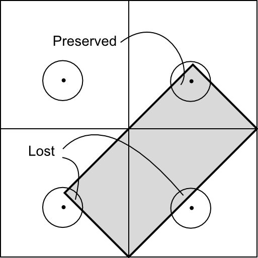
Figure 2.— Boundary effects and Smoothed Particles. Four images of a particle intersecting the boundary are shown. The top-right image is contained in the transformed domain, but the other three are not. The contribution of the two bottom images is lost. By requiring the size of the transformed domain to be much larger than typical SPH smoothing lengths, most particles do not intersect a boundary of the domain and the error is contained near the edges.

Table 1Transformations

Simulation	MassiveBlack	E5
Matrix $M$	$\left[\begin{smallmatrix}5&6&2\\ 3&-7&3\\ 2&7&0\end{smallmatrix}\right]$	$\left[\tiny\begin{smallmatrix}3&1&0\\ 2&1&0\\ 0&2&1\end{smallmatrix}\right]$
$R_{11}$(h-1Mpc)	3300	180
$R_{11}$ Pixels(Kilo)	810	36.57
$R_{22}$(h-1Mpc)	5800	101
$R_{22}$ Pixels(Kilo)	1440	20.48
$R_{33}$(h-1Mpc)	7.9	6.7
Resolution(h-1Kpc)	4.2	4.9

4. Rasterization

In a simulation, many field variables are of interest in visualization.

• scalar fields : density $\rho$, temperature $T$, neutral fraction $x_{\text{HI}}$, star formation rate $\phi$;

• vector fields: velocity, gravitational force.

In an SPH simulation, a field variable as a function of spatial position is given by the interpolation of the particle properties. Rasterization converts the interpolated continuous field into raster pixels on a uniform grid. The kernel function of a particle at position $\mathbf{y}$ with smoothing length $h$ is defined as

$$W(\mathbf{y},h)=\frac{8}{\pi h^{3}}\begin{cases}1-6\left(\frac{y}{h}\right)^{2}+6&\left(\frac{y}{h}\right)^{3},0\leq\frac{y}{h}\leq\frac{1}{2}\\ 2\left(1-\frac{y}{h}\right)^{3},&\frac{1}{2}<\frac{y}{h}\leq 1,\\ 0&\frac{y}{h}>1.\end{cases}$$

Following the usual prescriptions (e.g. Springel, 2005; Price, 2007), the interpolated density field is taken as

$$\rho(\mathbf{x})=\sum_{i}m_{i}W(\mathbf{x}-\mathbf{x}_{i},h_{i}),$$

where $m_{i}$, $\mathbf{x}_{i}$, $h_{i}$ are the mass, position, and smoothing length of the $i$th particle, respectively. The interpolation of a field variable, denoted by $A$, is given by

$$A(\mathbf{x})=\sum_{i}\frac{A_{i}m_{i}W(\mathbf{x}-\mathbf{x}_{i},h_{i})}{\rho(\mathbf{x}_{i})}+O(h^{2}),$$

where $A_{i}$ is the corresponding field property carried by the $i$th particle. Note that the density field can be seen as a special case of the general formula.

Two types of pixel-wise mean for a field are calculated, the

1. volume-weighted mean of the density field,

   $$\bar{\rho}(P) =\frac{M(P)}{P}=\frac{1}{P}\int_{P}d^{3}\mathbf{x}\,\rho(\mathbf{x})$$

   $$=\frac{1}{P}\sum_{i}m_{i}\int_{P}d^{3}\mathbf{x}\,W(\mathbf{x}-\mathbf{x}_{i},h_{i})$$

   $$=\frac{1}{P}\sum_{i}M_{i}(P),$$

   where $M_{i}(P)=m_{i}\int_{P}d^{3}\mathbf{x}\,W(\mathbf{x}-\mathbf{x}_{i},h_{i})$ is the mass overlapping of the $i$th particle and the pixel, and the

2. mass-weighted mean of a field ($A$) ,

   $$\bar{A}(P) = \frac{\int_{P}d^{3}\mathbf{x}\,A(\mathbf{x})\rho(\mathbf{x})}{\int_{P}d^{3}\mathbf{x}\,\rho(\mathbf{x})}$$

   $$= \frac{\sum_{i}A_{i}M_{i}(P)}{M(P)}+O(h^{2}).$$

To obtain a line of sight projection along the third axis, the pixels are chosen to extend along the third dimension, resulting a two dimensional final raster image. The calculation of the overlapping $M_{i}(P)$ in this circumstance is two dimensional. Both formulas require frequent calculation of the overlap between the kernel function and the pixels. An effective way to calculate the overlap is via a lookup table that is pre-calculated and hard coded in the program. Three levels of approximation are used in the calculation of the contribution of a particle to a pixel:

1. When a particle is much smaller than a pixel, the particle contributes to the pixel as a whole. No interpolation and lookup occurs.

2. When a particle and pixel are of similar size of (up to a few pixels in size), the contribution to each of the pixels are calculated by interpolating between the overlapping areas read from a lookup table.

3. When a particle is much larger than a pixel, the contribution to a pixel taken to be the center kernel value times the area of a pixel.

Note that Level 1 and 3 are significantly faster than Level 2 as they do not require interpolations.

The rasterization of the $z=4.75$ snapshot of MassiveBlack was run on the SGI UV Blacklight supercomputer at the Pittsburgh Supercomputing Center. Blacklight is a shared memory machine equipped with a large memory for holding the image and a fairly large number of cores enabling parallelism, making it the most favorable machine for the rasterization. The rasterization of the E5 simulation was run on local CMU machine Warp. The pixel dimensions of the raster images are also listed in Table 1. The pixel scales have been chosen to be around the gravitational softening length of $\sim 5\,\mathrm{h^{-1}Kpc}$ in these simulations in order to preserve as much information in the image as possible.

5. Image Rendering and Layer Compositing

The rasterized SPH images are color-mapped into RGBA (red, green, blue and opacity) layers. Two modes of color-mapping are implemented, the simple mode and the intensity mode.

In the simple mode, the color of a pixel is directly obtained by looking up the normalized pixel value in a given color table. To address the large (several orders of magnitude) variation of the fields, the logarithm of the pixel value is used in place of the pixel value itself.

In the intensity mode, the color of a pixel is determined in the same way as done in the simple mode. However, the opacity is reduced by a factor $f_{m}$ that is determined by the logarithm of the total mass of the SPH fluid contained within the pixel. To be more specific,

$$f_{m}=\begin{cases}0&\log M<a,\\ 1&\log M>b,\\ \left[\frac{\log M-a}{b-a}\right]^{\gamma}&\text{otherwise},\end{cases}$$

where $a$ and $b$ are the underexposure and overexposure parameters: any pixel that has a mass below $10^{a}$ is completely transparent, and any pixel that has a mass above $10^{b}$ is completely opaque.

The RGBA layers are stacked one on top of another to composite the final image. The compositing assumes an opaque black background. The formula to composite an opaque bottom layer $B$ with an overlay layer $T$ into the composite layer $C$ is (Porter & Duff, 1984)

$$C=\alpha F+(1-\alpha)T,$$

where $C$, $B$ and $T$ stand for the RGB pixel color triplets of the corresponding layer and $\alpha$ is the opacity value of the pixel in the overlay layer $T$. For example, if the background is red and the overlay color is green, with $\alpha=50\%$, the composite color is a $50\%$-dimmed yellow.

Point-like (non SPH) particles are rendered differently. Star particles are rendered as colored points, while black hole particles are rendered using circles, with the radius proportional to the logarithm of the mass. In our example images, the MassiveBlack simulation visualization used a fast rasterizer that does not support anti-aliasing, whilst the frames of E5 are rendered using matplotlib (Hunter, 2007) that does anti-aliasing.

The choice of the colors in the color map has to be made carefully to avoid confusing different quantities. We choose a color gradient which spans black, red, yellow and blue for the color map of the normalized gas density field. This color map is shown in Figure 3. Composited above the gas density field is the mass weighted average of the star formation rate field, shown in dark blue, and with completely transparency where the field vanishes. Additionally, we choose solid white pixels for the star particles. Blackholes are shown as green circles. In the E5 animation frames, the normalization of the gas density color map has been fixed so that the maximum and minimum values correspond to the extreme values of density in the last snapshot.

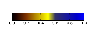
Figure 3.— Fiducial color-map for the gas density field. The colors span a darkened red through yellow to blue.

6. Parallelism and Performance

The large simulations we are interested in visualizing have been run on large supercomputer facilities. In order to image them with sufficient resolution to be truly useful, the creation of images from the raw simulation data also needs significant computing resources. In this section we outline our algorithms for doing this and give measures of performance.

6.1. Rasterization in parallel

We have implemented two types of parallelism, which we shall refer to as “tiny” and “huge”, to make best use of shared memory architectures and distributed memory architectures, respectively. The tiny parallelism is implemented with OpenMP and takes advantage of the case when the image can be held within the memory of a single computing node. The parallelism is achieved by distributing the particles in batches to the threads within one computing node. The raster pixels are then color-mapped in serial, as is the drawing of the point-like particles. The tiny mode is especially useful for interactively probing smaller simulations.

The huge version of parallelism is implemented using the Message Passing Interface (MPI) libraries and is used when the image is larger than a single computing node or the computing resources within one node are insufficient to finish the rasterization in a timely manner. The imaging domain is divided into horizontal stripes, each of which is hosted by a computing node. When the snapshot is read into memory, only the particles that contribute to the pixels in a domain are scattered to the hosting node of the domain. Due to the growth of cosmic structure as we move to lower redshifts, some of the stripes inevitably have many more particles than others, introducing load imbalance. We define the load imbalance penalty $\eta$ as the ratio between the maximum and the average of the number of particles in a stripe. The computing nodes with fewer particles tend to finish sooner than those with more. The color-mapping and the drawing of point-like particles are also performed in parallel in the huge version of parallelism.

6.2. Performance

The time spent in domain remapping scales linearly with the total number of particles $N$,

$$T_{\text{remap}}\sim O(N).$$

The time spent in color-mapping scales linearly with the total number of pixels $P$,

$$T_{\text{color}}\sim O(P).$$

Both processes consume a very small fraction of the total computing cycles.

The rasterization consumes a much larger part of the computing resources and it is useful to analyze it in more detail. If we let $\bar{n}$ be the number of pixels overlapping a particle, then $\bar{n}=K^{-1}N^{-1}P$, where $K^{-1}$ is a constant related to the simulation. Now we let $t(n)$ be the time it takes to rasterize one particle, as a function of the number of pixels overlapping the particle. From the 3 levels of detail in the rasterization algorithm (Section 4), we have

$$t(n)=\begin{cases}C_{1},&n\ll 1\\ C_{2}n&n\sim 1\\ C_{3}n,&n\gg 1\end{cases};$$

with $C_{2}\gg C_{1}\approx C_{3}$ . The effective pixel filling rate $R$ is defined as the total number of image pixels rasterized per unit time,

$$R=P[t(\bar{n)}N]^{-1}=\bar{n}K[t(\bar{n})]^{-1}$$

$$=\begin{cases}\bar{n}KC_{1}^{-1},&\bar{n}\ll 1\\ KC_{2}^{-1}&\bar{n}\sim 1\\ KC_{3}^{-1},&\bar{n}\gg 1\end{cases}.$$

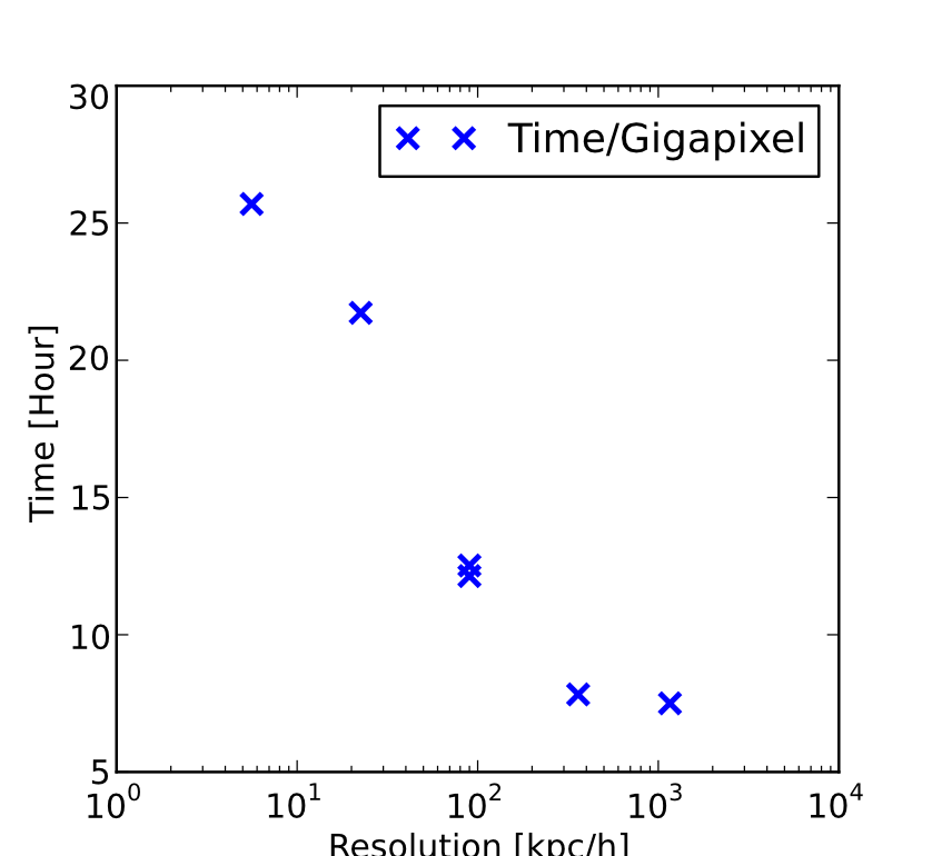
Figure 4.— MassiveBlack Simulation Rasterization Rate. We show the number of pixels fixed as a function of resolution (pixel scale). The rate peaks at $KC_{3}^{-1}$ at the high resolution limit and approaches $KC_{2}^{-1}$ as the resolution worsens. The $\bar{n}\ll 1$ domain is not explored.

The rasterization time to taken to create images from a single snapshot of the MassiveBlack simulation (at redshift 4.75) at various resolutions is presented in Table 2 and Figure 4.

Table 2Time Taken to Rasterize the MassiveBlack Simulation . Here $N$ is the number of SPH particles, Res is the resolution (pixel scale), $\overline{n}$ is mean number of pixels that overlap each particle, $\eta$ is the load unbalance penalty averaged over patches, and the final column, Rate, is the number of kilopixels rasterized per second.

Pixels	Res
($\mathrm{Kpc/px}$)	$\bar{n}$	CPUs	Wall-time
($\mathrm{hours}$)	$\eta$	Rate
($\mathrm{K/sec}$)
5.6G	58.4	80	128	1.63	1.45	11.3
22.5G	29.2	330	256	3.17	1.66	13.4
90G	14.6	1300	512	3.35	1.57	24.0
90G	14.6	1300	512	3.06	1.39	23.3
360G	7.3	5300	512	7.65	1.39	37.2
1160G	4.2	16000	1344	10.1	1.56	37.2

The rasterization of the images were carried out on Blacklight at PSC. It is interesting to note that for the largest images, the disk I/O wall-time, limited by the I/O bandwidth of the machine, overwhelms the total computing wall-time. The performance of the I/O subsystem shall be an important factor in the selection of machines for data visualization at this scale.

7. Image and Animation Viewing

Once large images or animation frames have been created, viewing them presents a separate problem. We use the GigaPan technology for this, which enables someone with a web browser and Internet connection to access the simulation at high resolution. In this section we give a brief overview of the use of the GigaPan viewer for exploring large static images, as well as the recently developed GigaPan Time Machine viewer for gigapixel animations.

7.1. Gigapan

Individual gigapixel-scale images are generally too large to be shared in easy ways; they are too large to attach to emails, and may take minutes or longer to transfer in their entirety over typical Internet connections. GigaPan addresses the problem of sharing and interactive viewing of large single images by streaming in real-time the portions of images actually needed by the viewer of the image, based on the viewers current area of focus inside the image. To support this real-time streaming, the image is divided up and rendered into small tiles of multiple resolutions. The viewer pulls in only the tiles needed for a given view. Many mapping programs (e.g., Google Maps) use the same technique.

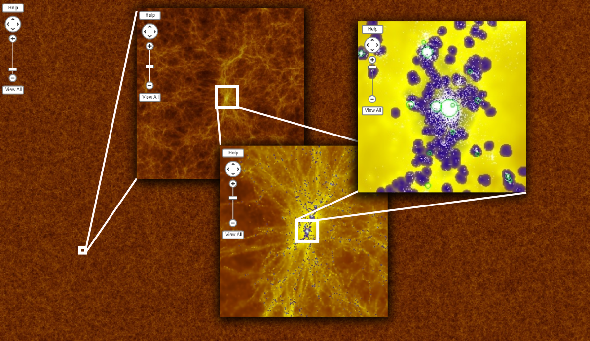
Figure 5.— GigaPan View of the MassiveBlack Simulation at $z=4.75$. The images are screen grab from the GigaPan viewer: we have left the magnification bar visible. The background is an overall view of the entire snapshot. We also show zooms into region around one of the most massive blackholes in the simulation, as shown in the right most zoom with the largest circle. The three zoom levels are $80\,\mathrm{h^{-1}Mpc}$, $8\,\mathrm{h^{-1}Mpc}$, $800\,\mathrm{h^{-1}Kpc}$, from left to right.

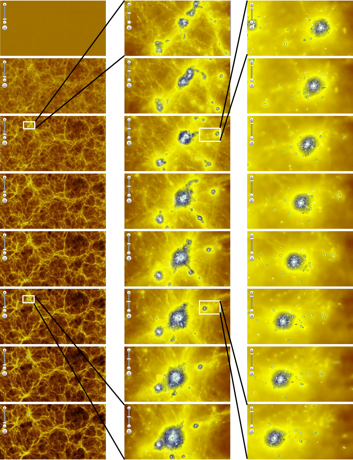
Figure 6.— GigaPan Time Machine Animation of the E5 simulation. These are screen grabs from the GigaPan Time Machine viewer. In the left column we show 8 frames (out of 1367 in the full animation) which illustrate the evolution of the entire simulation volume (at time intervals of $2\,\mathrm{Gyears}$. The middle panel zooms in to show formation of the largest halo through merger event. The right panel shows some of the history of a smaller halo.

We have uploaded an example terapixel image of the redshift $z=4.75$ snapshot of the MassiveBlack simulation to the GigaPan website, which is run as a publicly accessible resource for sharing and viewing large images and movies. The dimension of the image is $1440000\times 810000$, and the finished image uncompressed occupies $3.58\,\mathrm{TB}$ of storage space. The compressed hierarchical data storage in Gigapan format is about 15% of the size, or $0.5\,\mathrm{TB}$. There is no fundamental limits to size, provided the data can be stored on the disk. It is possible to create directly the compressed tiles of a GigaPan, bypassing the uncompressed image as an intermediate step, and thus reducing the requirement on memory and disk storage. We leave this for future work.

On the viewer side, static GigaPan works well at different bandwidths; the interface remains responsive independent of bandwidth, but the imagery resolves more slowly as the bandwidth is reduced. 250 kilobits/sec is a recommended bandwidth for exploring with a $1024\times 768$ window, but the system works well even when the bandwidth is lower.

An illustration of the screen output is shown in Figure 5. The reader is encouraged to visit the website to explore the image.

7.2. GigaPan Time Machine

In order to make animations, one starts with the rendered images of each individual snapshot in time. These can be gigapixel in scale or more. In our example, using the E5 simulation (Section 2.2) we have 1367 images each with 0.75 gigapixels.

One approach to showing gigapixel imagery over time would be to modify the single-image GigaPan viewer to animate by switching between individual GigaPan tile-sets. However, this approach is expensive in bandwidth and CPU, leading to sluggish updates when moving through time.

To solve this problem, we created a gigapixel video streaming and viewing system called GigaPan Time Machine (Sargent et al., 2010), which allows the user to fluidly explore gigapixel-scale videos across both space and time. We solve the bandwidth and CPU problems using an approach similar to that used for individual GigaPan images: we divide the gigapixel-scale video spatially into many smaller videos. Different video tiles contain different locations of the overall video stream, at different levels of detail. Only the area currently being viewed on a client computer need be streamed to the client and decoded. As the user translates and zooms through different areas in the video, the viewer scales and translates the currently streaming video, and over time the viewer requests from the server different video tiles which more closely match the current viewing area. The viewing system is implemented in Javascript+HTML, and takes advantage of recent browser’s ability to display and control videos through the new HTML5 video tag.

The architecture of GigaPan Time Machine allows the content of all video tiles to be precomputed on the server; clients request these precomputed resources without additional CPU load on the server. This allows scaling to many simultaneously viewing clients, and allows standard caching protocols in the browser and within the network itself to improve the overall efficiency of the system. The minimum bandwidth requirement to view videos without stalling depends on the size of the viewer, the frame rate, and the compression ratios. The individual videos in “Evolution of the Universe” (the E5 simulation, see below for link) are currently encoded at 25 FPS with relatively low compression. The large video tiles require a continuous bandwidth of 1.2 megabits/sec, and a burst bandwidth of 2.5 megabits/sec.

We have uploaded an example animation of the E5 simulation, showing its evolution over the interval between redshift $z=200$ and $z=0$ with 1367 frames equally spaced in time by 10 Myr. Again, the reader is encouraged to visit the website to explore the image.

8. Conclusions

We have presented a framework for generating and viewing large images and movies of the formation of structure in cosmological SPH simulations. This framework has been designed specifically to tackle the problems that occur with the largest datasets. In the generation of images, it includes parallel rasterization (for either shared and distributed memory) and adaptive pixel filling which leads to a well behaved filling rate at high resolution. For viewing images, the GigaPan viewers use hierarchical caching and cloud based storage to make even the largest of these datasets fully explorable at high resolution by anyone with an internet connection. We make our image making toolkit publicly available, and the GigaPan web resources are likewise publicly accessible.

References

- Abazajian (2003) Abazajian K. et, al, 2003, AJ, 126, 2081
- Boylan-Kolchin et al. (2009) Boylan-Kolchin M., Springel V., White S. D. M., Jenkins A., and Lemson G., 2009, MNRAS, 398, 1150
- Bryan & Norman (1997) Bryan G. L. & Norman M. L., 1997, ASP Conference Series, 123, 363
- Carlson & White (2010) Carlson J. & White M., 2010, ApJS, 190, 311-314
- Colberg et al. (2005) Colberg J. M., Krughoff K. S., and Connolly A. J., 2005, MNRAS, 359, 272
- Degraf et al. (2011, in prep) Degraf C. et al., 2011 in preparation
- Dekel et al. (2009) Dekel A., Birnboim Y., Engel G. Freundlich J., Mumcuoglu M., Neistein E., Pichon C., Teyssier R., and Zinger E., 2009, Nature, 456, 451
- Di Matteo et al. (2008) Di Matteo T., Colberg J., Springel V., Hernquist L., and Sijacki D., 2008, ApJ, 676, 33-53.
- Di Matteo et al. (2005) Di Matteo T., Springel V., and Hernquist L., 2005, Nature, 433, 604
- Di Matteo et al. (2011, in prep) Di Matteo et al., 2011, in preparation
- Dolag et al. (2006) Dolag K., Meneghetti M., Moscardini L., Rasia E., and Bonaldi A., 2006, MNRAS, 370, 656
- Fraedrich et al. (2009) Fraedrich R., Schneider J., and Westermann R., 2009, IEEE Transactions on Visualization and Computer Graphics 15(6), 1251-1258
- Gnedin (2011) Gnedin, N., http://sites.google.com/site/ifrithome/Home
- Hernquist & Springel (2003) Hernquist L. & Springel V., 2003, MNRAS, 341, 1253
- Hilbert et al. (2009) Hilbert S., Hartlap J., White S.D.M, and Schneider P., 2009, å, 499,31
- Hunter (2007) Hunter J. D., 2011, Computing in Science & Engineering, 9, 3, 90
- Jenkins et al. (1998) Jenkins A. et al., 1998, ApJ, 499, 20
- Keres et al. (2005) Keres D., Katz N., Weinberg D., and Dave R., 2005, MNRAS, 363, 2
- Khandai et al. (2011, in prep) Khandai et al., 2011 in preparation
- Monaghan (1992) Monaghan J. J., 1992, ARA&A, 30, 543
- Porter & Duff (1984) Porter T. & Duff D. 1984, SIGGRAPH Comput. Graph. 18, 3, 253-259.
- Price (2007) Price D. J., 2007, Pub. of the Astro. Society of Australia, 24, 59-173
- Sargent et al. (2010) Sargent R., Bartley C., Dille P., Keller J., Nourbakhsh I., and LeGrand R., 2010, Fine Intl. Conf. on Gigapixel Imaging for Science
- Shin et al. (2008) Shin M., Tray H., and Cen R., 2008, ApJ, 681, 756
- Sijacki et al. (2007) Sijacki D., Springel V., Di Matteo T., and Hernquist L., 2007, MNRAS, 380, 877
- Springel et al. (2001) Springel V., Yoshida N., and White S. D. M., 2005, New Astronomy, 6, 2, 79
- Springel (2005) Springel V., 2005, MNRAS, 364, 1105
- Springel et al. (2005) Springel V., et al. 2005, Nature, 435, 629
- Szalay et al. (2008) Szalay T., Springel V.,Lemson G., 2008 Microsoft eScience Conference. arXiv:0811.2055
- Turk et al. (2011) Turk M. J., Smith, B. D., Oishi J. S., Skory S., Skillman S. W., Abel T., and Norman M., 2011, ApJS, 192, 9.
- Wadsley et al. (2004) Wadsley J. W., Stadel J., and Quinn T., 2004, New Astronomy, 9, 137
- Zahn et al. (2007) Zahn O., Lidz A., McQuinn M., Dutta S., Hernquist L., Zaldarriage M., and Furlanetto S. R., 2007, ApJ, 654, 12