Homogeneous studies of transiting extrasolar planets.
IV. Thirty systems with space-based light curves

Abstract

I calculate the physical properties of 32 transiting extrasolar planet and brown-dwarf systems from existing photometric observations and measured spectroscopic parameters. The systems studied include fifteen observed by the CoRoT satellite, ten by Kepler and five by the Deep Impact spacecraft. Inclusion of the objects studied in previous papers leads to a sample of 58 transiting systems with homogeneously measured properties. The Kepler data include observations from Quarter 2, and my analyses of several of the systems are the first to be based on short-cadence data from this satellite.

The light curves are modelled using the jktebop code, with attention paid to the treatment of limb darkening, contaminating light, orbital eccentricity, correlated noise, and numerical integration over long exposure times. The physical properties are derived from the light curve parameters, spectroscopic characteristics of the host star, and constraints from five sets of theoretical stellar model predictions. An alternative approach using a calibration from eclipsing binary star systems is explored and found to give comparable results whilst imposing a much smaller computational burden.

My results are in good agreement with published properties for most of the transiting systems, but discrepancies are identified for CoRoT-5, CoRoT-8, CoRoT-13, Kepler-5 and Kepler-7. Many of the errorbars quoted in the literature are underestimated. Refined orbital ephemerides are given for CoRoT-8 and for the Kepler planets. Asteroseismic constraints on the density of the host stars are in good agreement with the photometric equivalents for HD 17156 and TrES-2, but not for HAT-P-7 and HAT-P-11.

Complete error budgets are generated for each transiting system, allowing identification of the observations best-suited to improve measurements of their physical properties. Whilst most systems would benefit from further photometry and spectroscopy, HD 17156, HD 80606, HAT-P-7 and TrES-2 are now extremely well characterised. HAT-P-11 is an exceptional candidate for studying starspots. The orbital ephemerides of some transiting systems are becoming uncertain and they should be re-observed in the near future.

The primary results from the current work and from previous papers in the series have been placed in an online catalogue, from where they can be obtained in a range of formats for reference and further study. TEPCat is available at http://www.astro.keele.ac.uk/$\sim$jkt/tepcat/

1 Introduction

Of the 550 planets known to orbit stars other than our Sun, the transiting systems are the most interesting ones. Transiting extrasolar planets (TEPs) are the only planets outside our Solar system whose masses and radii, and thus surface gravities and mean densities, can be measured to reasonable precision. Observational selection effects mean that most known TEPs orbit very close to their parent star and thus have highly irradiated atmospheres whose physical properties can be scrutinised using high-quality astronomical observations.

One hindrance to the study of TEPs is that measurement of their physical properties requires not only transit light curves and radial velocity measurements of the parent stars, but also some sort of additional constraint. This is ordinarily obtained by forcing the properties of the star to match predictions from theoretical stellar models, guided by an effective temperature ($T_{\rm eff}$) and metal abundance ($\left[\frac{\rm Fe}{\rm H}\right]$) obtained from spectral analysis. The dependence on stellar theory leads to systematic errors which can be sizeable for some of the measured quantities, and also allows inhomogeneities to occur between studies which use different theoretical predictions or apply the constraint in a different way. This in turn compromises statistical studies of transiting planets.

For these reasons I am measuring the properties of the known TEPs using strictly homogeneous methods. Paper I (Southworth, 2008) discussed the methodology used to model the transit light curves, paying particular attention to error analysis and the treatment of limb darkening, and applied them to the 14 systems with good observational data at the time. Paper II (Southworth, 2009) explored the application of constraints from seven different sets of theoretical model predictions and alternatively an empirical mass–radius relation obtained from eclipsing binaries. Three of the sets of theoretical predictions were selected to aid in the determination of the physical properties of the same 14 systems, with detailed error budgets including random and systematic contributions. In Paper III (Southworth, 2010) I extended the number of systems to 30 and the number of theoretical predictions used to five sets, improving both the statistical weight of the ensemble and the precision of the systematic errorbars.

In the current work I enlarge the number of TEPs with homogeneous properties to 58, concentrating on those which have been observed by the space missions Kepler (Borucki et al., 2010b), CoRoT (Baglin et al., 2006) and EPOCH (Christiansen et al., 2009). In Paper II I outlined the concept of applying an observational mass–radius relation instead of using constraints from stellar theory, resulting in totally empirical measurements of the properties of TEP systems. This approach was not very successful (see Paper III) because the mass-radius relation did not allow for stellar evolution and had to be calibrated on low-mass eclipsing binary systems whose properties (primarily radius) are affected by magnetic activity arising from comparatively fast rotation. In the current work I follow the alternative approach of Enoch et al. (2010) which relates the radius of the star to its density, $T_{\rm eff}$ and $\left[\frac{\rm Fe}{\rm H}\right]$. This technique is not purely empirical, as it incorporates parameters derived using spectral synthesis techniques for both the TEP hosts and the calibrating sample, but returns results in much better agreement with the default method using theoretical predictions. Finally, I explore the opportunities for further study of the systems studied in this work.

For a small number of TEPs it is possible to either partially or totally avoid systematic errors: the study of transit timing variations (TTVs) allow the masses of some TEPs to be constrained directly (Holman & Murray, 2005; Lissauer et al., 2011); and radial velocities of the planet HD 209458 b have been measured by Snellen et al. (2010a) from infrared absorption lines, allowing the system properties to be calculated in an identical way to double-lined eclipsing binary star systems. These methods are, however, not applicable to the predominant population of TEPs which show no detectable TTVs and are not amenable to direct velocity measurements.

2 Analysis of the light curves

I have modelled the light curves of each TEP using the methods espoused in Paper I. In short, the jktebop code (Southworth et al., 2004a, b) is used to model the available transit light curves. The components are approximated as biaxial spheroids whose shapes are governed by the mass ratio, $q$. The results in this work are all extremely insensitive to the values adopted for $q$.

The main parameters of a jktebop fit are the orbital inclination, $i$, and the fractional radii of the star and planet, $r_{\rm A}$ and $r_{\rm b}$. These are defined as

$$r_{\rm A}=\frac{R_{\rm A}}{a}\qquad\qquad r_{\rm b}=\frac{R_{\rm b}}{a}$$ (1)

where $R_{\rm A}$ and $R_{\rm b}$ are the volume-equivalent stellar and planetary radii and $a$ is the orbital semimajor axis. In jktebop the fractional radii are re-parameterised as their sum and ratio:

$$r_{\rm A}+r_{\rm b}\qquad\qquad k=\frac{r_{\rm b}}{r_{\rm A}}=\frac{R_{\rm b}}{R_{\rm A}}$$ (2)

as these are less strongly correlated. In general the orbital period, $P_{\rm orb}$, is taken from the literature and the time of transit midpoint, $T_{0}$, is included as a fitted parameter.

Each light curve is fitted with a number of different approaches to limb darkening (LD). 1$\sigma$ errorbars are obtained using 1000 Monte Carlo simulations (Southworth et al., 2004c, 2005b). Errorbars are also calculated using a residual permutation (or “prayer bead”) algorithm (Jenkins et al., 2002) which accounts for correlated observational noise, and the largest of the two alternatives is adopted for each parameter.

The LD of the star has an important influence on transit light curves. For each light curve, solutions are obtained using five different LD laws, each with three different approaches to the limb darkening coefficients (LDCs): (1) both fixed (hereafter ‘LD-fixed’); (2) the linear one ($u_{\rm A}$) fitted and the nonlinear one ($v_{\rm A}$) fixed but perturbed by $\pm$0.05 in the error analysis simulations (‘LD-fit/fix’); and (3) both coefficients fitted (‘LD-fitted’). Initial or fixed values for the LDCs are bilinearly interpolated in $T_{\rm eff}$ and $\log g$ within the tabulated theoretical predictions included in the jktld code.

Once the best of the three alternatives (LD-fixed, LD-fit/fix, LD-fitted) is identified, the combined solution for that option is calculated by taking the mean of the solutions for the four two-coefficient LD laws and by taking the largest errorbar from these solutions plus a contribution to account for the scatter in the parameter values. In most cases the LD-fit/fix solutions turn out to be the best compromise between severing the dependence on theoretical calculations and trying to fit too many parameters to the data.

Some TEPs have a non-circular orbit which changes the duration of the transit but has a negligible effect on the light curve shape (Kipping, 2008). I account for this by adding published constraints on orbital eccentricity ($e$) and periastron longitude ($\omega$), with the parameter combinations $e\cos\omega$ and $e\sin\omega$ when possible, using the approach outlined in Paper III and Southworth et al. (2009c).

An additional annoyance for some systems is light from a nearby star contaminating the photometry (e.g. Daemgen et al., 2009). This ‘third light’ makes the transit shallower but cannot be fitted for in the light curve due to strong degeneracy with $r_{\rm A}$, $r_{\rm b}$ and $i$ (see Paper III). When third light is known to exist it is accounted for using the method put forward by Southworth et al. (2010).

2.1 Numerical integration of light curves

Figure 1: Parameters of light curve solutions of an undersampled light curve, closely resembling that of Kepler-6, with different numbers of numerical integration points used in the solution. Unbroken lines show the correct parameter values and dotted lines show the $\pm$1% intervals for these parameters.

Figure 2: Plot of a model light curve closely resembling that of Kepler-6, but covering 32 instead of 12 orbital periods (blue points). This is compared to the best fit obtained without using numerical integration (red line). The residuals of the fit are plotted at the base of the figure offset from zero.

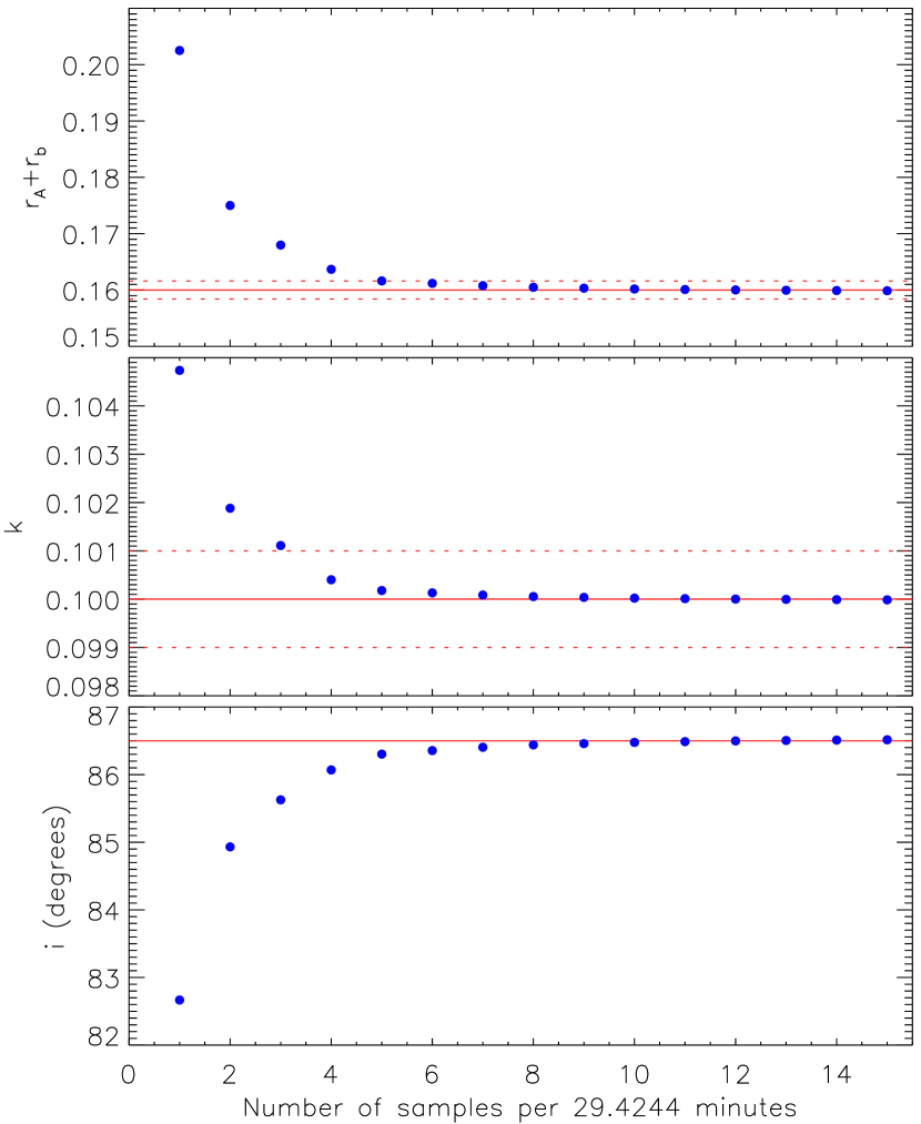
In some light curves the sampling rate is a significant fraction of the transit duration, leading to a smearing of the transit shape. If left uncorrected this could cause errors of up to 30% (worst-case scenario) in the physical properties of TEPs. The prime candidates for this problem are the Kepler planets, whose long-cadence photometric points consist of summations of 270 consecutive datapoints leading to an overall sampling rate of one datum every 29.4244 min (Jenkins et al., 2010b). Some of the CoRoT satellite data are also affected, as the standard cadence for this instrument is 512 s. Most CoRoT TEPs also have short-cadence sampling with a rate of 32 s; these data do not suffer from temporal undersampling.

For the current work I have modified jktebop to optionally perform numerical integration to cope with the Kepler and CoRoT data. The approach is to calculate a given number of model datapoints ($N_{\rm int}$) evenly spread over a given time interval, and sum them to create an integrated datapoint which can be directly compared with observations. The next question is: how fine a time sampling is necessary? I created a dataset very similar to that of the TEP Kepler-6 by generating a model light curve ($r_{\rm A}+r_{\rm b}=0.16$, $k=0.10$, $i=86.5^{\circ}$, quadratic LD), extending it over 12 orbital cycles, and summing it into 29.4 min bins. This was then fitted with $N_{\rm int}$ varied from 1 (i.e. no numerical integration) to 15 (equivalent to a 1.96 min sampling rate). The resulting values of $r_{\rm A}+r_{\rm b}$, $k$ and $i$ are plotted in Fig. 1 and show that $r_{\rm A}+r_{\rm b}$ is more affected than $k$ and $i$. Using $N_{\rm int}=10$ means we incur an error of only 0.1% in $r_{\rm A}+r_{\rm b}$; using $N_{\rm int}=5$ would engender a 1% error. TEPs with shorter orbital periods (i.e. quicker transits) or higher $i$ (sharper partial phases) will be more strongly affected.

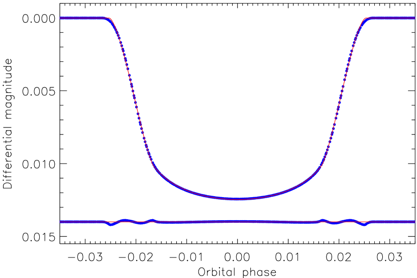
Fig. 2 shows the Kepler-6-like model light curve extended to cover 32 orbital cycles and summed into 29.4 min bins. This has been fitted by jktebop but without performing numerical integration, in order to demonstrate the effect of neglecting the undersampling. The fitted model is unable to correctly reproduce the synthetic data during the partial phases of the transit, the discrepancy being worst at the first and last contact points where the light curve derivative is of greatest magnitude. This suggests that it would be possible to fit for the amount of numerical integration needed for a high-quality dataset, although it is very unlikely that such an option will ever be useful. The amount of numerical integration needed will also be quite sensitive to LD, particularly around the limb of the star.

3 Calculation of physical properties

3.1 Via stellar models

Analysis of a transit light curve gives the quantities $P_{\rm orb}$, $T_{0}$, $r_{\rm A}$, $r_{\rm b}$ and $i$. Radial velocity (RV) measurements of the parent star yield its orbital velocity amplitude, $K_{\rm A}$. Measuring the physical properties of the system requires an additional constraint, which is normally taken from theoretical stellar evolutionary models. The observed stellar effective temperature, $T_{\rm eff}$ and metal abundance, $\left[\frac{\rm Fe}{\rm H}\right]$, are useful to guide this process, which is discussed in detail in Paper II and Paper III.

I use the velocity amplitude of the planet ($K_{\rm b}$) to control the solution process. A starting value is guessed, and is combined with the measured $P_{\rm orb}$, $r_{\rm A}$, $r_{\rm b}$, $i$ and $K_{\rm A}$ to obtain the physical properties of the system using standard formulae (e.g. Hilditch, 2001). The resulting calculated stellar mass ($M_{\rm A}$) and measured $\left[\frac{\rm Fe}{\rm H}\right]$ are used to obtain the expected stellar radius ($R_{\rm A}$) and $T_{\rm eff}$ by interpolation in a set of tabulated theoretical predictions. $K_{\rm b}$ is then iteratively refined to obtain the best agreement with the calculated $R_{\rm A}$ and observed $T_{\rm eff}$ by minimising the figure of merit:

$${\rm fom}=\left[\frac{r_{\rm A}^{\rm(obs)}-(R_{\rm A}^{\rm(calc}/a)}{\sigma{\rm(r_{\rm A}^{\rm(obs)})}}\right]^{2}+\left[\frac{T_{\rm eff}^{\rm(obs)}-T_{\rm eff}^{\rm(pred)}}{\sigma(T_{\rm eff}^{\rm(obs)})}\right]^{2}$$ (3)

This process is performed for a range of ages from the zero-age to the terminal-age main sequence (curtailed at a maximum of 20 Gyr) to find the overall best fit. The code which performs this step (jktabsdim) has been profiled in order to improve its speed, which has allowed the step size in age to be decreased from 0.1 Gyr to 0.01 Gyr for the current work.

The uncertainties on the input parameters to jktabsdim are propagated using a perturbation analysis (Southworth et al., 2005a), resulting in a complete error budget for every output parameter. This allows identification of which type of observations would be best to improve our understanding of each TEP (see Sect. 9).

Apart from the random errors, which are calculated using the propagation analysis, systematic errors arise from the use of theoretical stellar models. These can be estimated by running solutions with a range of different model predictions. As in Paper III I use five sets of model predictions: Claret (Claret, 2004, 2005, 2006, 2007), Y² (Demarque et al., 2004), Teramo (Pietrinferni et al., 2004), VRSS (VandenBerg et al., 2006) and DSEP (Dotter et al., 2008). jktabsdim is run with each of these five sets, and the final results are taken to be the unweighted mean of the individual values for each output quantity. The statistical error is taken to be the largest of the individual uncertainties from the perturbation analysis, and the systematic error to be the standard deviation of the values from each of the model sets. The final results therefore rest evenly on the predictions of all five model sets. Since Paper III I have obtained additional tabulations for the Claret models, for fractional metal abundances of $Z=0.005$ and $Z=0.015$, to allow for $\left[\frac{\rm Fe}{\rm H}\right]$ values down to $-0.60$. I have also identified and fixed a mistake in my reformatting of the VRSS models which caused the wrong $M_{\rm A}$ values to be used for a small number of tabulations.

The final results from five runs of jktabsdim with different theoretical model sets is the following parameters with statistical and systematic errorbars: the mass, radius, surface gravity and density of the star ($M_{\rm A}$, $R_{\rm A}$, $\log g_{\rm A}$, $\rho_{\rm A}$) and of the planet ($M_{\rm b}$, $R_{\rm b}$, $g_{\rm b}$, $\rho_{\rm b}$). In additional to this I calculate a surrogate for the equilibrium temperature for the planet:

$$T_{\rm eq}^{\,\prime}=T_{\rm eff}\left(\frac{R_{\rm A}}{2a}\right)^{1/2}=T_{\rm eff}\left(\frac{r_{\rm A}}{2}\right)^{1/2}$$ (4)

and also its Safronov (1972) number:

$$\Theta=\frac{1}{2}\left(\frac{V_{\rm esc}}{V_{\rm orb}}\right)^{2}=\left(\frac{a}{R_{\rm b}}\right)\left(\frac{M_{\rm b}}{M_{\rm A}}\right)=\frac{1}{r_{\rm b}}\frac{M_{\rm b}}{M_{\rm A}}$$ (5)

Three quantities are independent of stellar theory: $g_{\rm b}$ (Southworth et al., 2007b), $\rho_{\rm A}$ (Seager & Mallén-Ornelas, 2003) and $T_{\rm eq}^{\,\prime}$ (Paper III).

3.2 Via eclipsing binary relations

Table 1: Coefficients of the equations for $\log_{10}M$ and $\log_{10}R$ derived using eclipsing binary star systems. Extra significant figures are provided to guard against round-off errors.

Calibration parameter	$\log_{10}M$		$\log_{10}M$		$\log_{10}R$		$\log_{10}R$
Valid mass range ($\,{\rm M}_{\odot}$)	0.2 to 27.0		0.2 to 3.0		0.2 to 27.0		0.2 to 3.0
$c_{1}$	0.01092 $\pm$	0.00176	0.01384 $\pm$	0.00263	0.003759 $\pm$	0.000933	0.007055 $\pm$	0.000930
$c_{2}$	1.0826 $\pm$	0.0178	1.0569 $\pm$	0.0268	0.36325 $\pm$	0.00711	0.37796 $\pm$	0.00729
$c_{3}$	0.4028 $\pm$	0.0259	0.360 $\pm$	0.107	0.1317 $\pm$	0.0102
$c_{4}$	$-$0.15139 $\pm$	0.00536	$-$0.16236 $\pm$	0.00936	$-$0.38296 $\pm$	0.00161	$-$0.37880 $\pm$	0.00175
$c_{5}$	$-$0.0008 $\pm$	0.00159	$-$0.01405 $\pm$	0.00589
$c_{6}$	0.1803 $\pm$	0.0105	0.1755 $\pm$	0.0102	0.06020 $\pm$	0.00417	0.06004 $\pm$	0.00422
Scatter (dex)	0.0286		0.0268		0.00953		0.00907

In Paper II I found a way to bypass the use of stellar models entirely, by defining an empirical mass–radius relation based on well-studied and unevolved detached eclipsing binary star systems (dEBs). The chief advantages of this approach were tractability and the avoidence of a dependence on stellar theory. The primary disadvantage was that the results were much inferior to those calculated using stellar models. This arose because the known well-studied dEBs tend to have substantially larger radii than predicted by the models (see e.g. López-Morales 2007; Ribas et al. 2008), so a more massive star was needed to reproduce the density obtained from the light curve solutions. Stellar evolution was also not allowed for, so the systems with more evolved stars were found to be rather more massive than they actually are. These problems make a simple mass–radius relation untenable.

An alternative approach would be to use the empirical relations for dEBs defined by Torres et al. (2010), which give $\log M$ and $\log R$ in terms of $\log T_{\rm eff}$, $\log g$ and $\left[\frac{\rm Fe}{\rm H}\right]$. These account for evolution and also for metal abundance, and have a modest scatter of $\sigma=0.027$ in $\log M$ and $\sigma=0.014$ in $\log R$. As noted by Enoch et al. (2010), a better approach for TEPs would be to replace $\log g$ with $\log\rho$ as the former quantity is rather tricky to derive from spectra of solar-like stars, whereas the latter quantity is almost directly measurable from transit light curves (Seager & Mallén-Ornelas, 2003). Enoch et al. (2010) found that this modified approach yields lower scatters of $\sigma=0.023$ in $\log M$ and $\sigma=0.009$ in $\log R$.

There are several possible criticisms of the implementation of this method by Enoch et al. (2010). Firstly, they included only those dEBs with metallicity measurements (19 out of the 95 systems in the compilation by Torres et al. 2010) so could suffer from small-number statistics. Also, many of the TEP host stars are of mass $\la$1.3$\,{\rm M}_{\odot}$ where metal abundance has a much smaller effect on the stellar properties. Secondly, they included component stars of dEBs with masses up to 15$\,{\rm M}_{\odot}$, which are of uncertain value for studying the currently know TEP hosts. Finally, a plot of density versus $T_{\rm eff}$ does not allow one to conclude that the dEBs are good calibrators of TEP host stars: the former might be systematically less dense than the latter (see Fig. 3). This leads to concerns that the relations have to be extrapolated to TEP hosts rather than interpolated. However, the Enoch et al. (2010) approach yields results which are quick to calculate and are in good agreement with stellar theory, so is worthy of further investigation.

Figure 3: Plot of density versus $T_{\rm eff}$ for TEP host stars compared to well-studied dEBs. Filled (red) circles represent data from Paper III and the current work and open circles show data from the literature. Plusses and crosses (blue) denote the primary and secondary components of dEBs, respectively.

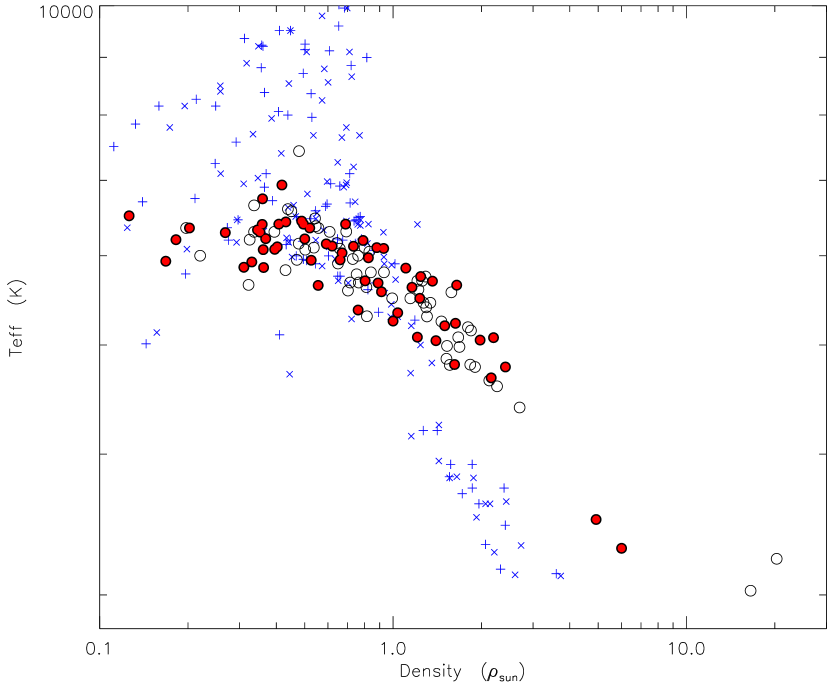
I have therefore obtained my own calibration of $\log_{10}M$ and $\log_{10}R$ in terms of $\log_{10}T_{\rm eff}$, $\log_{10}\rho$ and $\left[\frac{\rm M}{\rm H}\right]$. The calibration sample is taken from DEBCat and includes all stars but one with masses up to 3$\,{\rm M}_{\odot}$. Objects without a metallicity measurement were assigned $\left[\frac{\rm M}{\rm H}\right]=0\pm 100$. The final sample contains 90 dEBs (180 stars), and benefits in particular from the six new low-mass dEBs studied by Kraus et al. (2011).

The adopted equations are:

$$\log_{10}M = c_{1}+c_{2}\log_{10}X+c_{3}(\log_{10}X)^{2}$$ (6)

$$+c_{4}\log_{10}\rho+c_{5}(\log_{10}\rho)^{2}+c_{6}\left[\frac{\rm M}{\rm H}\right]$$

$$\log_{10}R = c_{1}+c_{2}\log_{10}X+c_{3}(\log_{10}X)^{2}$$ (7)

$$+c_{4}\log_{10}\rho+c_{5}(\log_{10}\rho)^{2}+c_{6}\left[\frac{\rm M}{\rm H}\right]$$

where $X=\log_{10}(T_{\rm eff}/T_{\rm eff,\odot})$, $T_{\rm eff,\odot}=5781$ K, and mass, radius and density are given in solar units. The coefficients of the fit, $c_{i}$, were found using a downhill simplex algorithm and are given in Table 1. The equation adopted for the current paper is for $\log_{10}R$ with a range of validity of 0.2–3.0$\,{\rm M}_{\odot}$. The scatter around the calibration is only 0.009 dex, in good agreement with Enoch et al. (2010). The coefficients are much more precise because of the larger calibration sample, but are not directly comparable because of a different choice of normalisation parameter for $T_{\rm eff}$. The calibration has been implemented into the jktabsdim code, and its scatter is propagated through into the final results using the perturbation method.

3.3 Constants and units

In previous papers in this series the densities of TEPs were given relative to that of Jupiter. The density of Jupiter was calculated incorrectly, using the equatorial radius rather than the volume-equivalent radius. The former is larger by 2.26% due to the oblateness of the planet, leading to a scale in which the density of the planet Jupiter was counterintuitively 1.0694$\,\rho_{\rm Jup}$. Starting with the present work I account for this effect, leading to planetary densities which are lower by 6.94%. No other quantities are affected by this oversight. In Table 2 I give the corrected densities of those planets which were studied in previous papers (see Paper III). It is likely that this error has occurred several times before in the literature, and in these cases $\rho_{\rm b}$ should be divided by 1.0694. In the Appendix I make no attempt to perform this correction to published values as it is not clear which of them are affected.

Table 2: Corrected planetary densities of the TEPs studied in Paper III.

System	$\rho_{\rm b}$ ($\,\rho_{\rm Jup}$)
GJ 436	$1.41^{+0.18}_{-0.02}$
HAT-P-1	$0.271^{+0.025}_{-0.002}$
HAT-P-2	$4.8^{+1.4}_{-0.0}$
HD 149026	$1.57\,^{+0.67}_{-0.53}\,{}^{+0.01}_{-0.01}$
HD 189733	$0.706\,^{+0.062}_{-0.062}\,{}^{+0.008}_{-0.008}$
HD 209458	$0.254^{+0.004}_{-0.002}$
OGLE-TR-10	$0.125^{+0.036}_{-0.000}$
OGLE-TR-56	$0.70^{+0.32}_{-0.32}$
OGLE-TR-111	$0.40^{+0.10}_{-0.00}$
OGLE-TR-113	$0.85^{+0.15}_{-0.01}$
OGLE-TR-132	$0.55^{+0.22}_{-0.00}$
OGLE-TR-182	$0.311^{+0.104}_{-0.002}$
OGLE-TR-211	$0.348\,^{+0.109}_{-0.124}\,{}^{+0.001}_{-0.001}$
OGLE-TR-L9	$0.96^{+0.35}_{-0.01}$
TrES-1	$0.536^{+0.052}_{-0.009}$
TrES-2	$0.584^{+0.048}_{-0.006}$
TrES-3	$0.804\,^{+0.047}_{-0.053}\,{}^{+0.006}_{-0.004}$
TrES-4	$0.138^{+0.037}_{-0.001}$
WASP-1	$0.246\,^{+0.055}_{-0.033}\,{}^{+0.001}_{-0.001}$
WASP-2	$0.70^{+0.13}_{-0.01}$
WASP-3	$0.63^{+0.10}_{-0.00}$
WASP-4	$0.463\,^{+0.014}_{-0.017}\,{}^{+0.005}_{-0.006}$
WASP-5	$0.93^{+0.13}_{-0.01}$
WASP-10	$2.43^{+0.36}_{-0.05}$
WASP-18	$6.21^{+0.84}_{-0.05}$
XO-1	$0.492^{+0.059}_{-0.005}$
XO-2	$0.532\,^{+0.111}_{-0.067}\,{}^{+0.012}_{-0.010}$
XO-3	$5.69^{+0.63}_{-0.06}$
XO-4	$0.66\,^{+0.12}_{-0.37}\,{}^{+0.01}_{-0.00}$
XO-5	$0.79^{+0.17}_{-0.00}$

This seems an appropriate point to specify the values of all constants and adopted quantities used in the present series of papers. The measured physical properties of the star are given in solar units for mass, radius and mean density, and in c.g.s. for $\log g$. For the planet, mass, radius and density are given in Jupiter units, and surface gravity in  m s^-2. Table 3 gives all constants used, plus the ensuing values of some quantities of interest. Since this paper was submitted, Harmanec & Prša (2011) have proposed a standardisation of the physical constants used in astronomy. They propose that a nominal solar mass, radius and luminosity are defined as exact quantities for use by all researchers. The values they propose are in full agreement with those used in the current work.

Table 3: Physical constants and adopted quantities used in the current work. The lower part of the Table gives the value of several quantities resulting from the adopted physical constants.
References: (1) US National Institute of Standards and Technology (2006 constants); (2) IERS Conventions 2010 (Petit & Luzum, 2010); (3) 2010 Astronomical Almanac; (4) Brown & Christensen-Dalsgaard (1998); (5) Bahcall et al. (1995); (6) JPL DE405 Ephemerides; (7) NASA NSSDC Jupiter fact sheet.

Parameter	Value	Unit	Ref.
Stefan-Boltzmann constant	$5.67040\times 10^{-8}$	W m-2 K-4	1
$G$	$6.67428\times 10^{-11}$	m3 kg-1 s-1	1
$GM_{\odot}$	$1.32712421\times 10^{20}$	m3 s-2	2
AU	$1.49597871\times 10^{11}$	m	3
$R_{\odot}$	$6.95508\times 10^{9}$	m	4
$L_{\odot}$	$3.844\times 10^{26}$	W	5
$R_{\rm Jup}$ (equatorial)	$7.1492\times 10^{8}$	m	3
$M_{\odot}$/$M_{\rm Jup}$	$1.0473486\times 10^{3}$		6
Volume of Jupiter	$1.43128\times 10^{24}$	m3	7
$M_{\odot}$	$1.98842\times 10^{30}$	kg
$\log g_{\odot}$	$4.43831$	(c.g.s.)
$\rho_{\odot}$	$1410.95$	kg m-3
$M_{\rm Jup}$	$1.89852\times 10^{27}$	kg
$g_{\rm Jup}$ (equatorial)	$24.7916$	m s-2
$\rho_{\rm Jup}$	$1326.45$	kg m-3

4 Light curve morphology

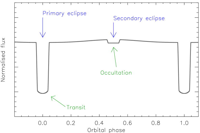
The literature contains a proliferation of terms for the different types of eclipses in TEP systems. The correct terminology has been established for many years for eclipsing binary systems (e.g. Hilditch, 2001) – and a TEP is simply a special case of an eclipsing binary. A ‘transit’ is when a smaller object passes in front of a larger object, for example a planet in front of a star. An ‘occultation’ is when a smaller object passes behind a larger object. Transits and occultations are two types of eclipses, and the third type is a ‘partial eclipse’. Fig. 4 is a schematic representation of the situation.

The definition of ‘primary eclipse’ is when the hotter object is behind the cooler object, and ‘secondary eclipse’ denotes to the reverse situation. This ordinarily means that the primary eclipse is deeper than the secondary, although exceptions to the rule are possible in the case of eccentric orbits (where different surface areas are covered at the two types of eclipse). For almost all TEPs, primary eclipses are transits and secondary eclipses are occultations.

Eclipsing systems can have only one transit per orbit, so references to a ‘primary transit’ or ‘anti-transit’ are misleading. The phrase ‘secondary transit’ is incorrect and should not be used.

Table 4: Parameters from the light curve analyses presented here and in previous works, and used here to determine the physical properties of the TEPs. The orbital periods are either from this work or from the literature, and the bracketed numbers represent the uncertainty in the preceding digits. Systems for which orbital eccentricity or third light was accounted for are indicated with a $\star$ in the column marked “$e$?” or “$L_{3}$?”, respectively.

System	Orbital period	$e$?	$L_{3}$?	Orbital inclination,		Fractional stellar		Fractional planetary		Reference
	(days)			$i$ (degrees)		radius, $r_{\rm A}$		radius, $r_{\rm b}$
CoRoT-1	1.5089686 (6)		$\star$	84.42 $\pm$	0.31	0.2073 $\pm$	0.0020	0.02924 $\pm$	0.00041	This work
CoRoT-2	1.7429935 (10)	$\star$	$\star$	87.45 $\pm$	0.34	0.1478 $\pm$	0.0023	0.02462 $\pm$	0.00035	This work
CoRoT-3	4.2567994 (35)		$\star$	85.80 $\pm$	0.77	0.1266 $\pm$	0.0067	0.00857 $\pm$	0.00056	This work
CoRoT-4	9.20205 (37)		$\star$	$89.96^{+0.04}_{-0.79}$		$0.0585^{+0.0046}_{-0.0015}$		$0.00608^{+0.00060}_{-0.00020}$		This work
CoRoT-5	4.0378962 (19)	$\star$	$\star$	86.24 $\pm$	0.53	0.0977 $\pm$	0.0067	0.01129 $\pm$	0.00091	This work
CoRoT-6	8.886593 (4)		$\star$	88.88 $\pm$	0.25	0.0567 $\pm$	0.0013	0.00662 $\pm$	0.00019	This work
CoRoT-7	0.853585 (24)			79.6 $\pm$	3.2	0.264 $\pm$	0.039	0.0047 $\pm$	0.0012	This work
CoRoT-8	6.21229 (3)		$\star$	87.44 $\pm$	0.56	0.0659 $\pm$	0.0056	0.00537 $\pm$	0.00060	This work
CoRoT-9	95.2738 (14)	$\star$		89.97 $\pm$	0.13	0.01083 $\pm$	0.00072	0.001233 $\pm$	0.000089	This work
CoRoT-10	13.2406 (2)	$\star$	$\star$	88.57 $\pm$	0.18	0.0326 $\pm$	0.0023	0.00424 $\pm$	0.00038	This work
CoRoT-11	2.994330 (11)		$\star$	83.13 $\pm$	0.19	0.1452 $\pm$	0.0022	0.01549 $\pm$	0.00023	This work
CoRoT-12	2.828042 (13)		$\star$	85.79 $\pm$	0.43	0.1235 $\pm$	0.0035	0.01638 $\pm$	0.00074	This work
CoRoT-13	4.035190 (30)		$\star$	85.27 $\pm$	0.47	0.1161 $\pm$	0.0053	0.01173 $\pm$	0.00063	This work
CoRoT-14	1.51214 (13)		$\star$	79.7 $\pm$	1.4	0.206 $\pm$	0.019	0.0181 $\pm$	0.0013	This work
CoRoT-15	3.06036 (3)		$\star$	$89.9^{+0.1}_{-5.0}$		$0.138^{+0.034}_{-0.009}$		$0.0109^{+0.0034}_{-0.0008}$		This work
HAT-P-4	3.0565195 (25)			$89.2^{+0.8}_{-1.5}$		$0.1666^{+0.0080}_{-0.0027}$		$0.01431^{+0.00072}_{-0.00028}$		This work
HAT-P-7	2.2047304 (24)			83.40 $\pm$	0.12	0.23880 $\pm$	0.00095	0.018401 $\pm$	0.000090	This work
HAT-P-11	4.88781501 (68)	$\star$		89.36 $\pm$	0.36	0.06148 $\pm$	0.00082	0.003604 $\pm$	0.000071	This work
HD 17156	21.216398 (16)	$\star$		86.94 $\pm$	0.34	0.04222 $\pm$	0.00079	0.003107 $\pm$	0.000081	This work
HD 80606	111.4367 (4)	$\star$		89.232 $\pm$	0.029	0.01056 $\pm$	0.00024	0.001045 $\pm$	0.000019	This work
Kepler-4	3.213658 (38)		$\star$	$89.2^{+0.8}_{-2.6}$		$0.153^{+0.026}_{-0.010}$		$0.00391^{+0.00076}_{-0.00034}$		This work
Kepler-5	3.548469 (15)		$\star$	$87.1^{+1.0}_{-0.6}$		$0.1445^{+0.0042}_{-0.0033}$		$0.01163^{+0.00032}_{-0.00027}$		This work
Kepler-6	3.2347020 (33)		$\star$	$89.9^{+0.1}_{-0.7}$		$0.1321^{+0.0017}_{-0.0006}$		$0.01259^{+0.00022}_{-0.00007}$		This work
Kepler-7	4.8854948 (82)		$\star$	85.31 $\pm$	0.43	0.1494 $\pm$	0.0035	0.01250 $\pm$	0.00041	This work
Kepler-8	3.5225047 (76)		$\star$	84.23 $\pm$	0.16	0.1432 $\pm$	0.0018	0.01360 $\pm$	0.00021	This work
KOI-428	6.87349 (64)			$86.5^{+3.5}_{-3.6}$		$0.139^{+0.029}_{-0.019}$		$0.0079^{+0.0021}_{-0.0013}$		This work
LHS 6343	12.71382 (4)	$\star$	$\star$	89.247 $\pm$	0.088	0.02388 $\pm$	0.00090	0.00489 $\pm$	0.00018	This work
TrES-2	2.47061323 (7)		$\star$	83.925 $\pm$	0.030	0.12568 $\pm$	0.00041	0.015979 $\pm$	0.000027	This work
TrES-3	1.30618700 (72)			81.93 $\pm$	0.13	0.1682 $\pm$	0.0014	0.02750 $\pm$	0.00035	This work
WASP-3	1.8468373 (14)			83.72 $\pm$	0.39	0.1994 $\pm$	0.0032	0.02125 $\pm$	0.00041	This work
WASP-7	4.9546416 (35)			87.03 $\pm$	0.93	0.1102 $\pm$	0.0061	0.01053 $\pm$	0.00070	Southworth et al. (2011)
XO-4	4.1250828 (40)			$89.9^{+0.1}_{-3.9}$		$0.1300^{+0.0283}_{-0.0051}$		$0.01124^{+0.00334}_{-0.00054}$		Paper III

Table 5: Measured quantities for the parent stars which were adopted in the analysis presented in this work.

System	Velocity amplitude ( m s-1)			$T_{\rm eff}$ (K)		Reference	$\left[\frac{\rm Fe}{\rm H}\right]$		Reference
CoRoT-1	188 $\pm$	11	Barge et al. (2008)	5950 $\pm$	150	Barge et al. (2008)	$-$0.30 $\pm$	0.25	Barge et al. (2008)
CoRoT-2	603 $\pm$	18	Gillon et al. (2010a)	5696 $\pm$	70	Chavero et al. (2010)	0.03 $\pm$	0.06	Chavero et al. (2010)
CoRoT-3	2170 $\pm$	27	Triaud et al. (2009)	6740 $\pm$	140	Deleuil et al. (2008)	$-$0.02 $\pm$	0.06	Deleuil et al. (2008)
CoRoT-4	63 $\pm$	6	Aigrain et al. (2008)	6190 $\pm$	60	Moutou et al. (2008)	0.05 $\pm$	0.07	Moutou et al. (2008)
CoRoT-5	$59.1^{+6.2}_{-3.1}$		Rauer et al. (2009)	6100 $\pm$	95	Rauer et al. (2009)	$-$0.25 $\pm$	0.06	Rauer et al. (2009)
CoRoT-6	280 $\pm$	30	Fridlund et al. (2010)	6090 $\pm$	70	Fridlund et al. (2010)	$-$0.20 $\pm$	0.10	Fridlund et al. (2010)
CoRoT-7	5.04 $\pm$	1.09	Hatzes et al. (2010)	5250 $\pm$	60	Bruntt et al. (2010)	0.12 $\pm$	0.06	Bruntt et al. (2010)
CoRoT-8	26 $\pm$	4	Bordé et al. (2010)	5080 $\pm$	80	Bordé et al. (2010)	0.31 $\pm$	0.05	Bordé et al. (2010)
CoRoT-9	38 $\pm$	3	Deeg et al. (2010)	5625 $\pm$	80	Deeg et al. (2010)	$-$0.01 $\pm$	0.06	Deeg et al. (2010)
CoRoT-10	301 $\pm$	10	Bonomo et al. (2010)	5075 $\pm$	75	Bonomo et al. (2010)	0.26 $\pm$	0.07	Bonomo et al. (2010)
CoRoT-11	280 $\pm$	40	Gandolfi et al. (2010)	6440 $\pm$	120	Gandolfi et al. (2010)	$-$0.03 $\pm$	0.08	Gandolfi et al. (2010)
CoRoT-12	$125.5^{+8.0}_{-7.5}$		Gillon et al. (2010b)	5675 $\pm$	80	Gillon et al. (2010b)	0.16 $\pm$	0.10	Gillon et al. (2010b)
CoRoT-13	157.8 $\pm$	7.7	Cabrera et al. (2010)	5945 $\pm$	90	Cabrera et al. (2010)	0.01 $\pm$	0.07	Cabrera et al. (2010)
CoRoT-14	1230 $\pm$	34	Tingley et al. (2011)	6035 $\pm$	100	Tingley et al. (2011)	0.05 $\pm$	0.15	Tingley et al. (2011)
CoRoT-15	7360 $\pm$	110	Bouchy et al. (2011)	6350 $\pm$	200	Bouchy et al. (2011)	0.1 $\pm$	0.2	Bouchy et al. (2011)
HAT-P-4	81.1 $\pm$	1.9	Kovács et al. (2007)	5860 $\pm$	80	Kovács et al. (2007)	0.24 $\pm$	0.08	Kovács et al. (2007)
HAT-P-7	211.8 $\pm$	2.6	Winn et al. (2009a)	6350 $\pm$	80	Pál et al. (2008)	0.26 $\pm$	0.08	Pál et al. (2008)
HAT-P-11	11.8 $\pm$	0.9	Hirano et al. (2011)	4780 $\pm$	50	Bakos et al. (2010)	0.31 $\pm$	0.05	Bakos et al. (2010)
HD 17156	272.7 $\pm$	2.1	Winn et al. (2009c)	6079 $\pm$	56	Fischer et al. (2007)	0.24 $\pm$	0.05	Fischer et al. (2007)
HD 80606	476.1 $\pm$	2.2	Winn et al. (2009b)	5574 $\pm$	72	Santos et al. (2004)	0.34 $\pm$	0.05	Gonzalez et al. (2010)
Kepler-4	$9.3^{+1.1}_{-1.3}$		Borucki et al. (2010a)	5857 $\pm$	120	Borucki et al. (2010a)	0.17 $\pm$	0.06	Borucki et al. (2010a)
Kepler-5	227.5 $\pm$	2.8	Koch et al. (2010)	6297 $\pm$	60	Koch et al. (2010)	0.04 $\pm$	0.06	Koch et al. (2010)
Kepler-6	80.9 $\pm$	2.6	Dunham et al. (2010)	5647 $\pm$	50	Dunham et al. (2010)	0.34 $\pm$	0.05	Dunham et al. (2010)
Kepler-7	42.9 $\pm$	3.5	Latham et al. (2010)	5933 $\pm$	50	Latham et al. (2010)	0.11 $\pm$	0.05	Latham et al. (2010)
Kepler-8	68.4 $\pm$	12.0	Jenkins et al. (2010a)	6213 $\pm$	150	Jenkins et al. (2010a)	$-$0.055 $\pm$	0.05	Jenkins et al. (2010a)
KOI-428	179 $\pm$	27	Santerne et al. (2011)	6510 $\pm$	100	Santerne et al. (2011)	$0.10^{+0.15}_{-0.10}$		Santerne et al. (2011)
LHS 6343	9600 $\pm$	300	Johnson et al. (2011)	3300 $\pm$	200	This work	0.04 $\pm$	0.08	Johnson et al. (2011)
TrES-2	181.3 $\pm$	2.6	O’Donovan et al. (2006)	5850 $\pm$	50	Sozzetti et al. (2007)	$-$0.15 $\pm$	0.10	Sozzetti et al. (2007)
TrES-3	369 $\pm$	11	Sozzetti et al. (2009)	5650 $\pm$	75	Sozzetti et al. (2009)	$-$0.19 $\pm$	0.08	Sozzetti et al. (2009)
WASP-3	286.5 $\pm$	7.8	This work	6400 $\pm$	100	Pollacco et al. (2008)	0.00 $\pm$	0.20	Pollacco et al. (2008)
WASP-7	97 $\pm$	13	Hellier et al. (2009b)	6400 $\pm$	100	Hellier et al. (2009b)	0.00 $\pm$	0.10	Hellier et al. (2009b)
XO-4	165.8 $\pm$	6.2	Narita et al. (2010)	6397 $\pm$	70	McCullough et al. (2008)	$-$0.04 $\pm$	0.05	McCullough et al. (2008)

5 Data acquisition

The CoRoT data used here are the N2 public version obtained from the public archive on 2010/12/03 (except for CoRoT-14 which was obtained on 2011/01/11) and interpreted using the N2 data description document. The CoRoT data are of two types: short-cadence and long-cadence. The total integration times for the two cadences are 32 s and 512 s, respectively. Many of the CoRoT TEPs have both types of data, and these are treated separately in each case.

Figure 4: Representation of a transit light curve with the main features indicated and labelled.

The Kepler data used are the public data obtained from the Multimission Archive at STScI (MAST). The Kepler quarter 0 (Q0) and quarter 1 (Q1) data were used in the original version of this work, but the analysis was revised to include quarter 2 (Q2) data when these became available. These data were downloaded from MAST on 2011/04/11. As with CoRoT, the Kepler data come in short-cadence and long-cadence flavours. The total integration times are 58.84876 s (Gilliland et al., 2010) and 29.4244 min (Jenkins et al., 2010b), respectively.

In order to account for slow variations in the mean flux level of the systems in the CoRoT and Kepler data (both astrophysical and instrumental), the data surrounding each transit were extracted from the full time-series and normalised to unit flux using a straight-line fit to the out-of-transit datapoints. In general the number of points used was roughly double the number in the transit, split equally before and after the transit. A straight line was used because it was adequate for the job and it cannot distort transit profiles. In a few cases entire transits were rejected because of a jump in observed flux during the transit or because the observations did not cover all of the transit event.

In cases where the number of datapoint was too large for Monte Carlo simulations to be completed in a reasonable length of time, the datasets were reduced down to a manageable size. This was done by converting the timestamps to orbital phase, sorting them, and then binning $N$ consecutive datapoints where $N$ ranged from 20 to 100. The value of $N$ was carefully chosen to ensure the sampling rate was still sufficiently high that numerical integration was not needed. The averaging process tends to convert correlated noise into white noise, but does not cause a problem for the error estimates of the resulting parameters. The phased and binned datapoints will be referred to as ‘normal points’ below, a term which was once used extensively in studies of eclipsing binaries. At the request of the referee I have analysed the CoRoT 32s-sampled data for CoRoT-1 both with and without phase-binning, in order to check that the binning process does not affect the solutions. The resulting light curve parameters differ by negligible amounts, supporting the use of phase-binning below.

6 Results for individual systems

In this section I present the photometric (jktebop) and absolute-dimensions (jktabsdim) analyses of 32 TEPs based on published high-quality data obtained from space missions, complemented with ground-based data where possible. The results are obtained using the same methods as those in Paper III, leading to homogeneous measurements for a sample of 58 TEPs. The final jktebop results of the 32 TEPs are collected in Table 4, which also includes the orbital periods and indicates for which systems a non-circular orbit was adopted. The adopted spectroscopic parameters ($T_{\rm eff}$, $\left[\frac{\rm Fe}{\rm H}\right]$ and $K_{\rm A}$) are given in Table 5, with a lower limit on the errorbars of $\pm$50 K for $T_{\rm eff}$ and $\pm$0.05 dex for $\left[\frac{\rm Fe}{\rm H}\right]$ (see Paper II). Extensive tables of results, plus a comparison with literature values, can be found in the online-only Appendix.

6.1 CoRoT-1

Figure 5: Phased light curves of CoRoT-1 compared to the best fit found using jktebop and the quadratic LD law. The residuals are plotted at the base of the figure, offset from unity. The purple line through some data show the best-fitting model without numerical integration – in these cases the difference between this model with and without numerical integration is shown by another purple line through the residuals. From top to bottom the light curves are the binned CoRoT 32 s data, the CoRoT 512 s data, the FORS2 $R$-band data and the FORS2 $B$-band data.

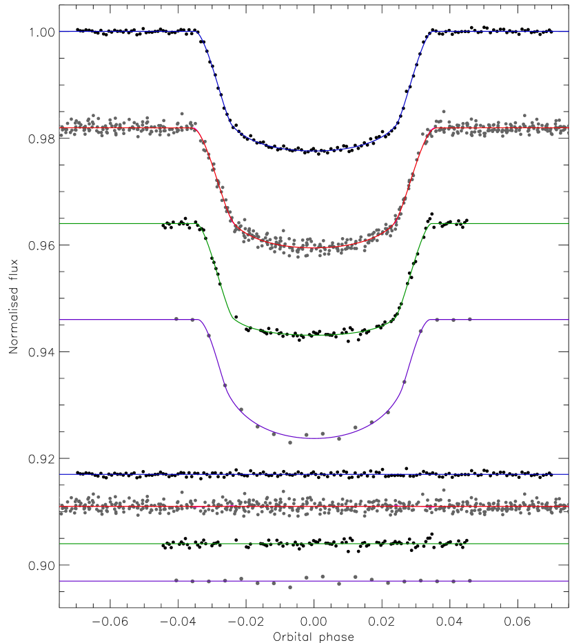
CoRoT-1 was the first TEP discovered by the CoRoT satellite (Barge et al., 2008), and was originally called CoRoT-Exo-1. The CoRoT data have been subjected to TTV analyses by Bean (2009) and Csizmadia et al. (2010) with null results. Gillon et al. (2009) observed a transit in the $R$-band using VLT/FORS2 and an occultation at 2.09 $\mu$m using VLT/HAWKI. The transit data are of very high precision (0.52 mmag scatter) but do not fully sample the transit. Pont et al. (2010) presented the same $R$-band data supplemented with a smaller number of $B$-band observations of the same transit taken with the same instrument. Pont et al. (2010) also obtained RV observations during a transit and detected a Rossiter-McLaughlin (RM) effect which show that the orbital axis of CoRoT-1 b is not aligned with the stellar spin axis. Occultation studies by Alonso et al. (2009b) and Rogers et al. (2009) and Deming et al. (2011) have found no evidence for orbital eccentricity, so I assumed that the orbit is circular.

The CoRoT data show 20 transits observed at long cadence (512 s) and 17 observed at short cadence (32 s). Each transit was normalised (Sect. 5) and the two cadences were treated separately in the jktebop analysis. After a preliminary fit the 32 s data were phase-binned with each phased datapoint representing 50 original ones. Seven out of 546 of the 512 s datapoints were rejected as 4$\sigma$ outliers. The 512 s data were modelled using numerical integration with $N_{\rm int}=3$. The $R$-band and $B$-band data were also studied (Fig. 5).

The results for the CoRoT 32 s data are given in Table A1 and are of sufficiently high quality for the LD-fitted solutions to be adopted. LD-fit/fix solutions were adopted for the CoRoT 512 s (Table A2) and the VLT $R$-band (Table A3) data, and in both cases correlated noise was found to be unimportant. Correlated noise is moderately important for the $B$-band data (the residual-permutation errorbars are larger than the Monte-Carlo errorbars) but the data were good enough to allow the LD-fit/fix solutions to be adopted (Table A4).

The photometric results are given in Table A5 and show good agreement except for $k$ (which has a reduced $\chi^{2}$ of $\chi_{\nu}^{\,2}=3.2$). This phenomenon has been noted several times before (Paper I, Paper II, Southworth et al. 2009b) and is attributable to correlated residuals (both instrumental and astrophysical) in the data. The $B$-band data cannot match their counterparts so I combine the other three sets of results together to get the final photometric parameters. These are in good agreement with those of the discovery paper (Barge et al., 2008) and of Bean (2009), but not with Gillon et al. (2009).

The physical properties of CoRoT-1 have been calculated using jktabsdim. The individual solutions are given in Table A6 and compared with literature values, where a good agreement is found (except for $\rho_{\rm A}$ from Gillon et al. 2009 due to their somewhat different photometric results). My measurements of $g_{\rm b}$, which is quite similar to the Earth’s surface gravity, and $\Theta$ appear to be the first ones published. Our understanding of the system would benefit from further spectroscopy to give improved values of $T_{\rm eff}$, $K_{\rm A}$ and $\left[\frac{\rm Fe}{\rm H}\right]$ in particular.

6.2 CoRoT-2

Figure 6: The 32 s light curve of CoRoT-2 compared to the jktebop best fit. Other comments are the same as Fig. 5.

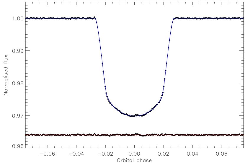
The discovery of CoRoT-2 was announced by Alonso et al. (2008) based on a 142 d light curve from the CoRoT satellite which exhibited transit events every 1.74 d and significant starspot activity on longer timescales. CoRoT-2 A is a young star hosting a relatively massive planet (3.6$\,{\rm M}_{\rm Jup}$). Bouchy et al. (2008) obtained RV measurements through transit and modelled the RM effect to find that the planetary orbital and projected stellar spin axes are aligned to within 7.2^∘ (1.6$\sigma$). The occultation of the planet has been found in the CoRoT data by Alonso et al. (2009a) and Snellen et al. (2010b), and its time of occurrence is consistent with a circular orbit. Gillon et al. (2010a) presented Spitzer observations of the secondary eclipse at 4.5 $\mu$m and 8 $\mu$m, finding a small but significant eccentricity characterised as $e\cos\omega=-0.00291^{+0.00063}_{-0.00061}$ and $e\sin\omega=0.0139^{+0.0079}_{-0.0084}$. Similar results have been obtained by Deming et al. (2011) from Warm-Spitzer observations at 3.6 $\mu$m: $e\cos\omega=-0.0030\pm 0.0004$.

The spot activity of CoRoT-2 A deserves mention. It is an active star with a rotation period of only 4.5 d and probable differential rotation (Lanza et al., 2009; Fröhlich et al., 2009; Huber et al., 2010; Silva-Valio & Lanza, 2011). One of the standard assumptions of modelling transit light curves of TEPs is that the surface brightness of those parts of the star eclipsed by the planet is the same as that of the rest of the star, modulo effects such as LD and gravity darkening. In the case of starspots this is certainly not a reliable assumption. However, the effect will average out over a large number of transits if the starspots do not show a preference for particular latitudes. But we know from the Sun that this is not the case: sunspots appear mostly within 30^∘ of the equator, and their preferred latitudes vary throughout the 11 yr solar activity cycle. A different effect is noticed in the study of active stars (e.g. Olah et al., 1997; Barnes, 2005) and eclipsing binaries, where light curve solutions often favour large polar spots (Hilditch, 2001). It is not usually possible to account for this problem in TEP studies because of the difficulty in detecting starspots outside the area eclipsed by the planet. The effect of starspots on the analysis of the CoRoT-2 system has been studied by Czesla et al. (2009) and Huber et al. (2010), who agree that the spot coverage on the chord of the planet transit is greater than the average for the stellar disc, and that the planet is therefore a few percent larger than standard analyses would suggest.

In the current work I have modelled the CoRoT 32 s light curve, which covers 79 transits. The 512 s data are not used as they only spread over three transits with partial coverage. 148 points of the 32 s data were rejected by a 4$\sigma$ clip and the remaining 50 666 points were phase-binned by a factor of 200 into 254 normal points. In the jktebop analysis I did not account for starspots, as this is beyond the scope of the current work, so have produced a baseline solution which is more easily comparable to the results for other TEPs. This is equivalent to assuming that the starspots affect all parts of the star equally on average. A third light of $L_{3}=0.053\pm 0.003$ (Alonso et al., 2008) and the small eccentricity (Gillon et al., 2010a) is accounted for in the ways described in Paper III. The VLT data from Gillon et al. (2010a) were not modelled because they only cover half a transit.

For the phase-binned 32 s data I found that correlated noise is not important and that the LD-fitted solutions are reliable enough to be adopted as the final photometric results (Table A7). A comparison with literature measurements (Table A8) shows an acceptable agreement except compared to the more sophisticated analysis of Czesla et al. (2009). My best fit to the 32 s data is plotted in Fig. 6.

The young age of CoRoT-2 (it is expected to be of Pleiades age) manifests itself in the jktabsdim analysis by the best solutions in some cases being on the zero-age edge of the grids of theoretical predictions. A modestly lower $T_{\rm eff}$ would alleviate this problem whilst not having a significant effect on the resulting physical properties. The edge effects can lead to underestimated errorbars for the affected solutions (see Paper II) but this is not a problem because the final results then rest on the errorbars from the unaffected solutions. The edge effect do, though, cause an increase in the systematic errorbars (Table A9).

CoRoT-2 A would benefit from an improved $T_{\rm eff}$ measurement: the discovery value of $5625\pm 120$ K (Alonso et al., 2008) is comparatively uncertain, the alternative measurement of $5608\pm 37$ K by Ammler-von Eiff et al. (2009) accompanies a $\log g$ which is too high (4.71 versus 4.53), and the value of $5696\pm 70$ K found by Chavero et al. (2010) is higher so causes stronger edge effects. A more precise measurement of $K_{\rm A}$ would be useful.

6.3 CoRoT-3

Figure 7: The 32 s (upper) and 512 s (lower) CoRoT light curves of CoRoT-3. Other comments are the same as Fig. 5.

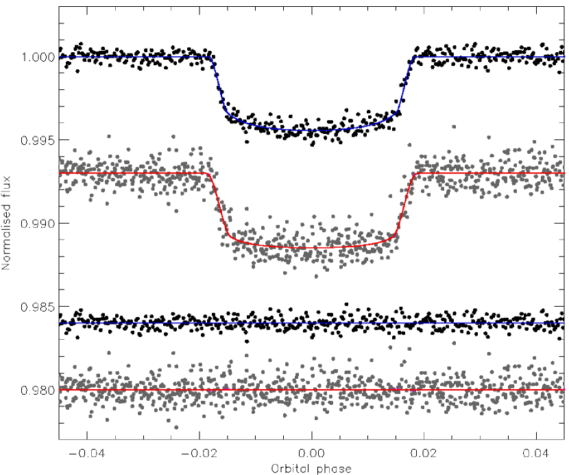
CoRoT-3 was announced by Deleuil et al. (2008) and was the first brown-dwarf-mass object with a precisely measured mass and radius. Its F3 V host star is rather hot (6740 K), making photometry and RV measurements difficult due to a shallow transit and high stellar $v\sin i$. An RM study has been presented by Triaud et al. (2009), whose measurements are consistent with a circular and axially aligned orbit.

The 32 s data cover 19 transits with a total of 196 691 datapoints. Of the 19 046 points in the regions of the transits, 20 were rejected by a 4$\sigma$ clip and the remainder were phase-binned by a factor of 40 to get 477 normal points. The 512 s data cover 16 transits and were fitted using $N_{\rm int}=3$. A circular orbit was assumed and a third light of $L_{3}=0.082\pm 0.007$ was adopted (Deleuil et al., 2008).

The results for the 32 s data are given in Table A10: correlated noise is not important (as usual for phase-binned datapoints) and the LD-fitted solutions yield the lowest scatter and reasonable LDCs. For the 512 s data (Table A11) correlated noise is again unimportant and the LD-fit/fix solutions are best. The best fits are plotted in Fig. 7. The final photometric parameters are the weighted means of the 32 s and 512 s values. They are compared to published values in Table A12, where a very good agreement is found.

The measured physical properties of CoRoT-3 are given in Table A13 and agree well with literature values. I provide the first measurement of $T_{\rm eq}^{\,\prime}$ and $\Theta$. The star could do with a better $T_{\rm eff}$ measurement, and an improved light curve would also be useful.

6.4 CoRoT-4

Figure 8: The 32 s (upper) and 512 s (lower) CoRoT light curves of CoRoT-4. Other comments are the same as Fig. 5.

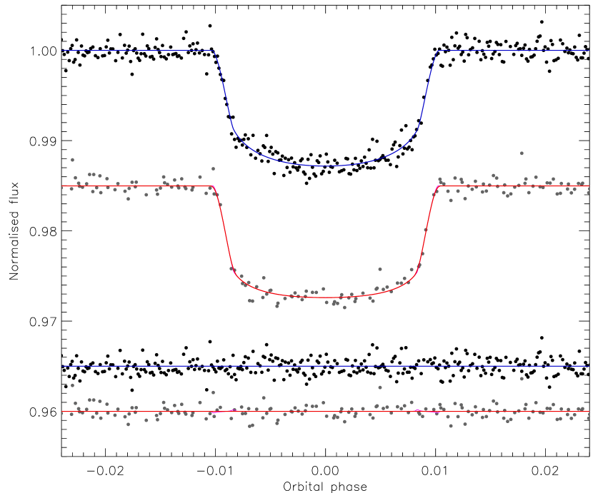
CoRoT-4 was discovered by Aigrain et al. (2008) and Moutou et al. (2008). It has a relatively long orbital period of 9.2 d, and thus one of the lower $T_{\rm eq}^{\,\prime}$s despite having a late-F host star. There are three transits each in the 32 s and the 512 s data. The 32 s data were phase-binned by a factor of 10 after 4$\sigma$ clipping to remove a small number of outliers. The 512 s data were modelled using $N_{\rm int}=3$.

The jktebop solutions favour a central transit, which causes the photometric parameters to have asymmetric errorbars. Correlated noise is unimportant for the phase-binned 32 s data but is important for the 512 s data. In both cases the LD-fit/fix results are the best (Tables A14 and A15). These were combined into final photometric parameters by multiplying their probability density functions (Table A16). The best fits are shown in Fig. 8. The agreement between my results and those of Aigrain et al. (2008) is excellent.

The physical properties of the CoRoT-4 system are given in Table A17 and show good agreement with those of Moutou et al. (2008) except for larger errorbars for some properties (notably $M_{\rm A}$ and $R_{\rm A}$). I provide the first published measurements of $\rho_{\rm A}$, $g_{\rm b}$ and $\Theta$. The long orbital period and short observing run conspire together to allow only six transits to be observed by CoRoT: a better light curve would be useful, as would a more precise $K_{\rm A}$.

6.5 CoRoT-5

Figure 9: The 32 s (upper) and 512 s (lower) CoRoT light curves of CoRoT-5. Other comments are the same as Fig. 5.

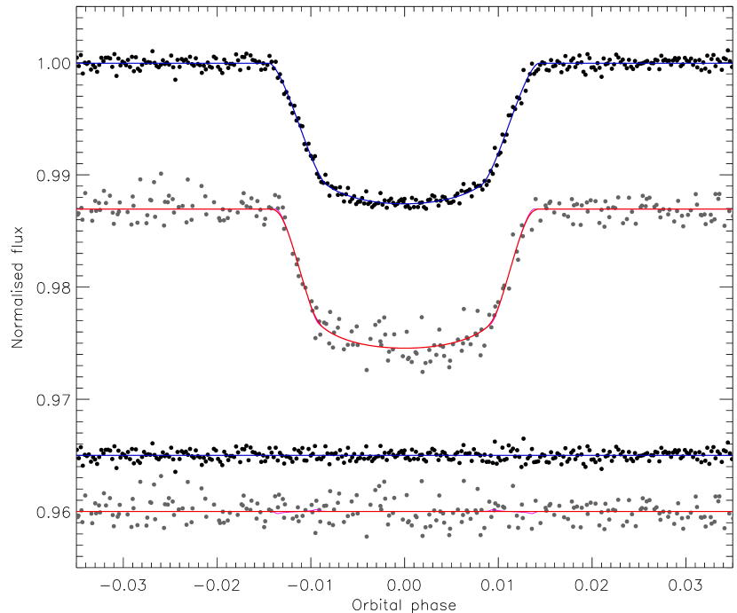
Discovered by Rauer et al. (2009), CoRoT-5 is a fairly normal system containing a low-density TEP. The 32 s data contain 23 transits, which were cut out of the light curve, 4$\sigma$ clipped and phase-binned as usual. The 512 s light curve contains six transits and these data were solved using $N_{\rm int}=3$. Rauer et al. (2009) found a preliminary third light of 8.6% (no uncertainty) so I adopted $L_{3}=0.086\pm 0.020$ for the jktebop analysis. Note that Rauer et al. (2009) removed this contaminating light from the light curve prior to modelling it, so neglected the uncertainty in $L_{3}$. Eccentricity is significant at the 3$\sigma$ level so this was included via the constraints $e\cos\omega=-0.057^{+0.048}_{-0.020}$ and $e\sin\omega=-0.071^{+0.147}_{-0.130}$.

The jktebop results are shown in Tables A18 and A19, and the best fits are plotted in Fig. 9. In both cases correlated noise was unimportant and the LD-fit/fix solutions were adopted. The two sets of results do not appear to agree very well, but are consistent to within 1$\sigma$. The errorbars are large primarily due to the poorly constrained orbital parameters: $e\cos\omega$ and $e\sin\omega$ are both uncertain and the latter is significantly correlated with $r_{\rm A}$ and $r_{\rm b}$. The combined results (Table A20) are in poor agreement with those of Rauer et al. (2009), presumably due to differences in the analysis methods.

The jktabsdim results are given in Table A21 and show a good agreement between the different model sets (and with the dEB constraint discussed in Sect. 3.2). As expected given the discrepant light curve results, I find physical properties which differ from those of Rauer et al. (2009) by up to 2$\sigma$. I find star and planet radii which are notably smaller than those of Rauer et al. (2009), and errorbars which are substantially larger (by a factor of 5 for $M_{\rm A}$). The properties of CoRoT-5 are more uncertain than previously thought, and additional RV measurements are the best route to fixing this.

6.6 CoRoT-6

Figure 10: The 32 s light curve of CoRoT-6. See Fig. 5 for details.

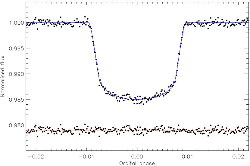
Comparatively speaking, CoRoT-6 is a massive (2.96$\,{\rm M}_{\rm Jup}$) and dense (1.66$\,\rho_{\rm Jup}$) TEP with a long orbital period (8.89 d) around a moderately active F9 V star. The discovery light curve from CoRoT (Fridlund et al., 2010) contains 331 397 datapoints at short cadence, covering 14 complete transits. A study of the starspot activity has been given by Lanza et al. (2011).

I adopted $e=0$ and $L_{3}=0.028\pm 0.007$ (Fridlund et al., 2010). 40 out of the 23 802 near-transit datapoints were rejected by a 4$\sigma$ clip and the remainder were phase-binned by a factor of 50 into 476 normal points. The jktebop results are given in Table A22 and are in good agreement with those of Fridlund et al. (2010). Correlated noise is completely negligible and the LD-fit/fix solution is the best choice (Table A23). The best fit is plotted in Fig. 10.

The physical properties of CoRoT-6 are given in Table A24, where the agreement between theoretical models, the dEB constraint and with Fridlund et al. (2010) is excellent. I provide the first measurements of $\rho_{\rm A}$, $g_{\rm b}$ and $\Theta$. The system could do with more spectroscopy to obtain an improved $K_{\rm A}$ and $\left[\frac{\rm Fe}{\rm H}\right]$.

6.7 CoRoT-7

Figure 11: The 32 s light curve of CoRoT-7. See Fig. 5 for details.

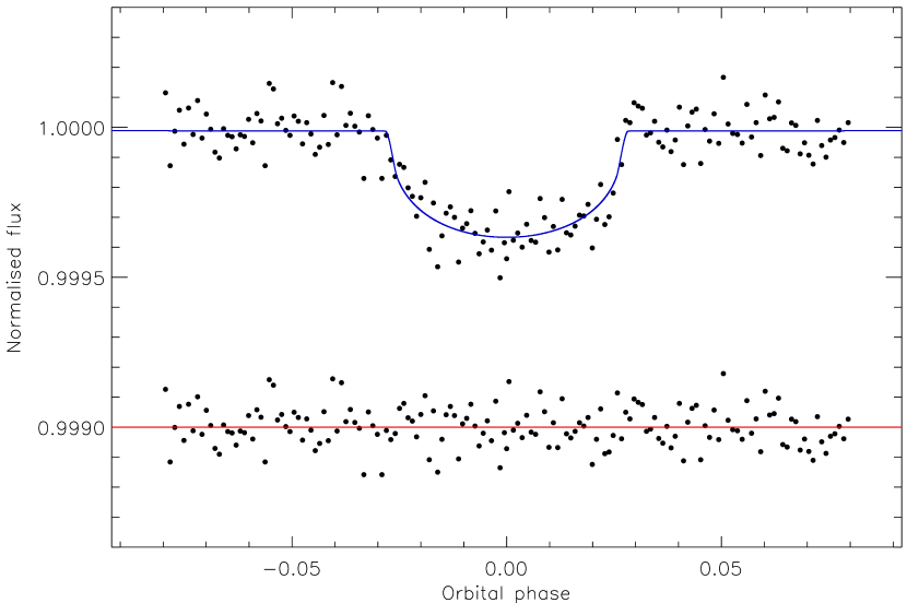
CoRoT-7 is one of the most important known planets. At the time of discovery it was both the smallest and least massive TEP discovered so far. The CoRoT light curve shows a transit of depth only 0.034% recurring on a period of only 0.85 d. A detailed analysis of these data, plus two high-precision RVs, proved the planetary nature of this object (Léger et al., 2009). Extensive RV measurements using the HARPS spectrograph (Queloz et al., 2009) confirmed the nature of the planet, with a mass of $4.8\pm 1.8$$\,{\rm M}_{\oplus}$, and allowed the discovery of a second one which is more massive (8.4$\,{\rm M}_{\oplus}$) and on a longer-period orbit (3.70 d). A study of the atmospheric parameters of the star by Bruntt et al. (2010) yielded a smaller $R_{\rm A}$ and therefore $R_{\rm b}$.

CoRoT-7 A is a G9 dwarf star with significant chromospheric activity. This activity causes larger RV variations that those of the planets’ orbits, making the properties of the system somewhat controversial. Lanza et al. (2010) studied the stellar activity and starspots and found a false-alarm probability of $<$10^-4 that the RV oscillations attributed to CoRoT-7 b and CoRoT-7 c are spurious effects of noise and activity. Hatzes et al. (2010) performed a comprehensive re-analysis of the RVs, finding a larger mass for CoRoT-7 b ($6.9\pm 1.4$$\,{\rm M}_{\oplus}$), confirming the RV signal of the second planet (CoRoT-7 c) and tentatively detecting a third RV signal which could be caused by another planet, CoRoT-7 d, with a mass of $16.7\pm 0.4$$\,{\rm M}_{\oplus}$ and a period of 9.02 d. However, Pont et al. (2011) performed a similar analysis, including a phenomenological model to describe the properties and evolution of many starspots, and found the RV signal of CoRoT-7 b to be a lot smaller and only significant at the 1.2$\sigma$ level ($M_{\rm b}=2.3\pm 1.5$$\,{\rm M}_{\oplus}$). The huge number of parameters in their starspot model could be expected to lead to more hazy results compared to those of other researchers. Ferraz-Mello et al. (2010) showed that previous analyses have tended to remove some of the planetary RV signal when squashing the effects of the stellar activity, and thus underestimate the masses. They found $M_{\rm b}=8.5\pm 1.5$$\,{\rm M}_{\oplus}$ and $M_{\rm c}\sin^{3}i_{\rm c}=13.5\pm 1.5$$\,{\rm M}_{\oplus}$, and that CoRoT-7 d is an artefact rather than an astrophysical signal. Boisse et al. (2011) also modelled the starspot-induced RV variations and confirmed planets b and c with false-alarm probabilities of $<5\times 10^{-4}$. They found masses of $M_{\rm b}=5.7\pm 2.5$$\,{\rm M}_{\oplus}$ and $M_{\rm c}\sin^{3}i_{\rm c}=13.2\pm 4.1$$\,{\rm M}_{\oplus}$. Just before the present paper was submitted, Hatzes et al. (2011) produced a re-analysis which confirmed their previous results for CoRoT-7 b. The difference in $K_{\rm A}$ ($5.15\pm 0.95$ m s^-1 versus $5.06\pm 1.06$ m s^-1) is so small that there was no need to recalculate my results.

The CoRoT light curve contains 308 947 datapoints, all at 32 s cadence. The 47 702 points near transits were phase-binned by a factor of 300 to give 160 normal points. The transit is so shallow (Fig. 11) that there was no point in calculating LD-fitted models. The results for the LD-fit/fix solutions (Table A25) show a good mutual agreement whereas the LD-fixed solutions do not. I therefore adopted the LD-fit/fix solutions. Compared to Léger et al. (2009), my results are in good agreement but have much larger errorbars (Table A26). This wraps over into the physical properties (Table A27). My analysis approach may not be optimal for this system, as I do not apply any external constraints to the light curve model (e.g. and spectroscopically derived $\log g$ or $\rho_{\rm A}$), but changing this would cause an inhomogeneity with the other TEPs treated in this work. CoRoT-7 would benefit from improved photometric and RV observations, although these are observationally highly demanding.

6.8 CoRoT-8

Figure 12: The 32 s (upper) and 512 s (lower) CoRoT light curves of CoRoT-8. Other comments are the same as Fig. 5.

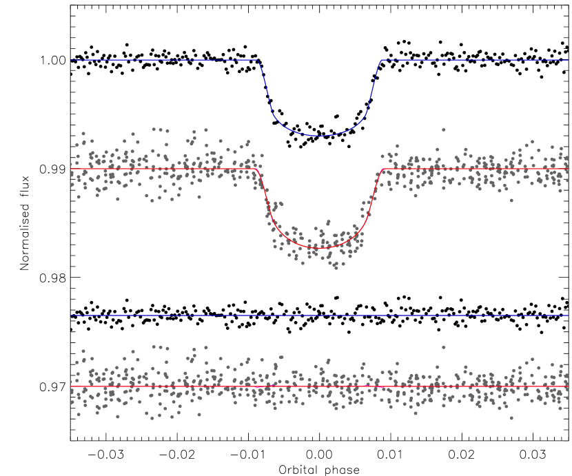
CoRoT-8 was discovered by Bordé et al. (2010) and is a small and low-mass planet in a relatively long-period orbit (6.21 d) around a metal-rich K dwarf. Bordé et al. (2010) quote a third light value of 0.9% without an errorbar; I adopted $L_{3}=0.009\pm 0.003$ in my photometric analysis. The 32 s data cover 12 transits with 19 413 datapoints. 46 were rejected by a 4$\sigma$ clip and the remainder were phase-binned by a factor of 40 to give 483 normal points. The 512 s observations harbour 11 transits; nine out of 946 points were rejected by a 4$\sigma$ clip and the remaining data were solved using $N_{\rm int}=3$.

In the course of extracting the transits from the CoRoT data it became clear that the ephemeris in Bordé et al. (2010) predicts transits to occur too early. I therefore binned up the 32 s data by a factor of 16 to match the 512 s data and fitted both datasets together to get a new orbital ephemeris:

$$T_{0}={\rm HJD}\,\,2\,454\,239.03311(78)\,+\,6.212381(57)\times E$$

where $E$ is the number of orbital cycles after the reference epoch and the bracketed quantities denote the uncertainty in the final digit of the preceding number. The errobars come from Monte Carlo and residual permutation simulations, which are in good agreement. Compared to the ephemeris of Bordé et al. (2010) I obtain larger errorbars, a consistent orbital period, and a $T_{0}$ which is later by 0.059 d (67$\sigma$). P. Bordé (private communication) has kindly confirmed that this discrepancy has been noted elsewhere, by two amateur astronomers who have found that the transits of CoRoT-8 occur later than predicted from the ephemeris in the discovery paper.

The 32 s and 512 s datasets were then fitted individually, the latter with $N_{\rm int}=3$. For both, correlated noise is unimportant and the LD-fit/fix solutions are adopted (Tables A28 and A29). The best fits are shown in Fig. 12. The combined solution of the two datasets (Table A30) does not agree well with the results of Bordé et al. (2010), in particular $r_{\rm A}$ (1.6$\sigma$) and $k$ (2.8$\sigma$). The errorbars found by Bordé et al. (2010) seem to be too small (e.g. 0.1^∘ compared to my 0.6^∘ for $i$), especially in light of the disagreement.

The physical properties of CoRoT-8 were not straightforward to derive. The long evolutionary timescale of the host star caused the best fits for the Teramo and VRSS models to be slightly discrepant with ages formally in excess of a Hubble time. However, reasonable solutions could be found by restricting the age range to 0–10 Gyr. My results (Table A31) again differ from those of Bordé et al. (2010), most obviously for the radii of the star ($0.90\pm 0.09$ versus $0.77\pm 0.02$) and planet ($0.71\pm 0.08$ versus $0.57\pm 0.02$). The masses of the components agree well with my results, and I present the first measurements of $g_{\rm b}$, $T_{\rm eq}^{\,\prime}$ and $\Theta$. I find that the density of the planet is less than half the value in the discovery paper. Further light curves and RVs would be useful for this object, in order to improve the system parameters and confirm the orbital ephemeris determined above.

6.9 CoRoT-9

Figure 13: The 32 s light curve of CoRoT-9. See Fig. 5 for details.

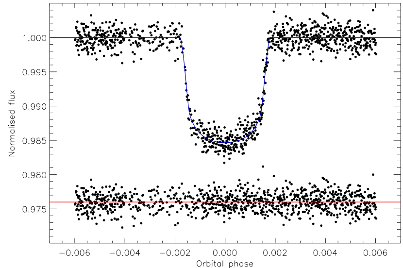
The discovery of the 93.7-d period CoRoT-9 system was announced by Deeg et al. (2010): the system has the longest $P_{\rm orb}$ of all TEPs bar HD 80606 (which was discovered in the course of an RV rather than a photometric survey). The CoRoT data cover only two transits of which one lacks coverage of ingress. The data were cut from the full light curve and phase-binned by a factor of 5 to yield 946 datapoints (Fig. 13). The orbital shape was constrained using $e=0.11\pm 0.04$ and $\omega=37^{+9}_{-37}$ (Deeg et al., 2010). The jktebop solutions show that correlated noise is not important and that the LD-fit/fix alternative is best (Table A32). The agreement with the results of Deeg et al. (2010) is excellent, both for the photometric parameters (Table A33) and the physical properties (Table A34). CoRoT-9 would benefit from further light curves and RVs.

6.10 CoRoT-10

Figure 14: The CoRoT 32s (upper) and 512s (lower) light curves of CoRoT-10. Other comments are the same as Fig. 5.

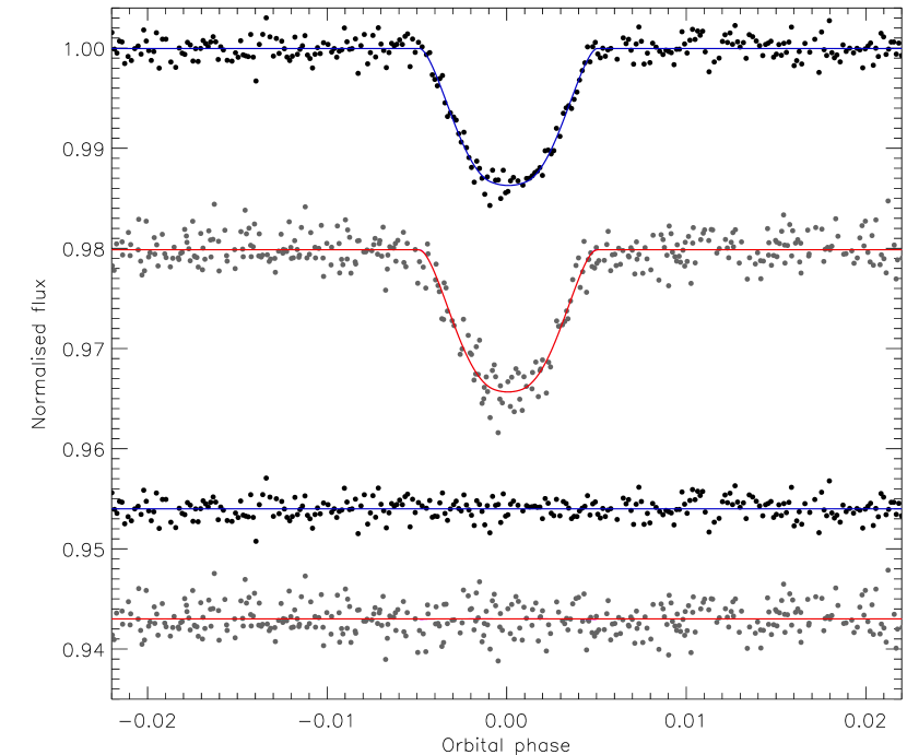
CoRoT-10 was discovered by Bonomo et al. (2010) and comprises a relatively massive TEP (2.78$\,{\rm M}_{\rm Jup}$) in a long-period (13.24 d) and highly eccentric ($e=0.53\pm 0.04$) orbit around a K1 dwarf. Five transits were observed at 512 s sampling and five more at 32 s sampling, of which one was ignored because it is affected by a data jump. A third light of $L_{3}=0.055\pm 0.003$ was found by Bonomo et al. (2010).

The 32 s data have 7190 points in the vicinity of a transit, of which 16 were rejected by a 4$\sigma$ clip and the rest phase-binned by a factor of 20 to give 369 normal points. No clipping or binning was needed for the 512 s data, which were solved using $N_{\rm int}=3$. The best fits are shown in Fig. 14 and the solutions arranged in Tables A35 and A36. My final photometric parameters (Table A37) agree well with those of Bonomo et al. (2010).

The physical properties of the system are not precisely defined (Table A38). It appears to be a young system, resulting in edge effects with the model grids (see CoRoT-2) and therefore larger systematic errorbars than is typical, especially for $M_{\rm A}$. However, the agreement with the Bonomo et al. (2010) parameters is good. A better light curve would be beneficial.

6.11 CoRoT-11

Figure 15: The CoRoT 32 s (upper) and 512 s (lower) light curves of CoRoT-11. Other comments are the same as Fig. 5.

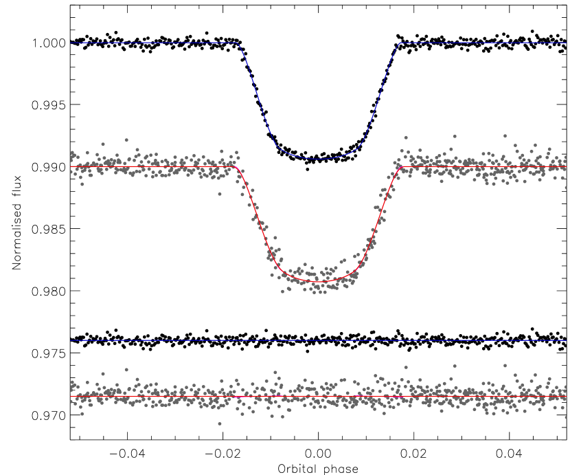
The star in the CoRoT-11 system is one of the earliest-type (F6 V) and most rapidly rotating ($40\pm 5$ km s^-1) TEP hosts known (Gandolfi et al., 2010). The planet itself is comparatively massive (2.34$\,{\rm M}_{\rm Jup}$) and has a high $T_{\rm eq}^{\,\prime}$ (1735 K). Gandolfi et al. (2010) found a third light of $L_{3}=0.130\pm 0.015$ which is included in the jktebop analysis.

The CoRoT 32 s data have 26 382 points near transits, of which 46 were rejected by a 4$\sigma$ clip and the rest phase-binned by a factor of 50 to get 527 normal points. The 512 s data contain 707 near transit of which 4 were rejected by a 4$\sigma$ clip and the remainder modelled using $N_{\rm int}=3$. For both light curves the LD-fit/fix solutions are the best and correlated noise is inconsequential (Tables A39 and A40). The fitted data are exhibited in Fig. 15. The results for the two datasets are unusual in that $k$ is the most consistent, whilst the other parameters agree to within less good 1.1$\sigma$. They were combined with this trifling disagreement accounted for in the errorbars. The final results are very similar to those of Gandolfi et al. (2010), and are among the better results for the known TEPs (TableA 41). This is helped by the relatively low $i$, which means the light curve fits are well-constrained.

The jktabsdim results for different model sets and for the dEB constraint (Table A42) agree well with each other and with Gandolfi et al. (2010). Further spectroscopic study of CoRoT-11 would be profitable.

6.12 CoRoT-12

Figure 16: The CoRoT 32 s (upper) and 512 s (lower) light curves of CoRoT-12. Other comments are the same as Fig. 5.

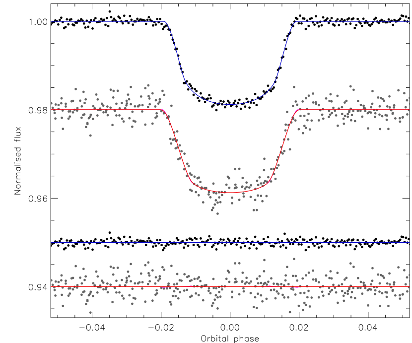
The discovery paper for the CoRoT-12 system (Gillon et al., 2010b) presents a system which is rather typical of the known population. The 32 s data comprise 242 558 datapoint of which 29 114 are adjacent to one of the 36 transits. A 4$\sigma$ clip discards 76 points and the remainder end up in 291 phase-binned normal points. The 512 s data cover 11 transits of which 413 points remain after rejecting 2780 which are away from eclipse and six which are over 4$\sigma$ away from a preliminary fit.

For the jktebop fits I adopted a circular orbit because the $e\cos\omega$ and $e\sin\omega$ values in Gillon et al. (2010b) are consistent with zero at the 1$\sigma$ level. A third light of $L_{3}=0.033\pm 0.005$ was used and $N_{\rm int}=3$ was employed for the 512 s data. The best fits are shown in Fig. 16 and the model solutions in Tables A43 and A44. In both cases correlated noise is unimportant and the LD-fit/fix solutions the most reliable. The results (Table A45) again show a slight disagreement between the two cadences, with $k$ the worst offender (1.7$\sigma$) and the other parameters divergent by an acceptable 1.2$\sigma$. The combined results agree reasonably well with those of Gillon et al. (2010b). A better light curve would be useful.

The final physical properties (Table A46) agree very well with Gillon et al. (2010b). Unusually, many of my error estimates are smaller than those found in the literature, which is attributable to the standard assumption of $e=0$ which neglects any uncertainty in the orbital shape. CoRoT-12 could do with further spectroscopic observations for both RV and spectral synthesis studies.

6.13 CoRoT-13

Figure 17: The CoRoT 32 s (upper) and 512 s (lower) light curves of CoRoT-13. Other comments are the same as Fig. 5.

Figure 18: Plot of the masses and radii of the known TEPs (dark blue crosses for those studied in this series of papers and light red crosses for other objects). The black open circle shows CoRoT-13 b (results from Cabrera et al. 2010) and the black filled circle shows CoRoT-13 b (results from this work). The grey dotted lines show the loci where density is equal to $\,\rho_{\rm Jup}$, $0.5\,\rho_{\rm Jup}$ and $0.25\,\rho_{\rm Jup}$.

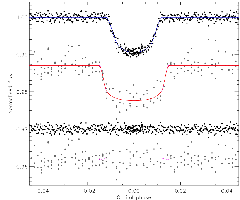
The discovery paper of this TEP is Cabrera et al. (2010). CoRoT observed 217 186 datapoints at 32 s cadence, covering 23 transits. Of the 22 020 points near transit, 54 were 4$\sigma$ clipped and the rest phase-binned by a factor of 50 to get 441 normal points. Of the 2403 512 s datapoints, 196 are near transit and were solved using $N_{\rm int}=3$. The quality of the 512 s light curve is relatively poor due to the faintness of the star. A third light of $L_{3}=0.11\pm 0.01$ was adopted from the discovery paper.

The best fits of the 32 s and the 512 s data are strikingly different (Fig. 17); I have verified that they arrived in the same datafile. The solutions for the 32 s data are in Table A47 and show that correlated noise is unimportant and that LD-fit/fix is to be preferred. Models with LDCs fixed at theoretical values have stronger LD and return $r_{\rm A}$ and $r_{\rm b}$ smaller by 1$\sigma$.

The 512 s light curve was difficult to model and suffered from instability of solution. This can be seen in most clearly by inspecting the inclination values in Table A48, which veer from grazing in the quadratic LD-fit/fix and square-root LD-fit/fix solutions to equatorial in the other 12 solutions. Other parameters are similarly affected. A greater consistency might be obtained by guiding the offending best fits towards the area of parameter space inhabited by the other best fits, but at the expense of mathematical rigour. A better idea is to reject the 512 s data, which are in any case of much lower weight than the much more extensive and better-sampled 32 s data. For my final photometric parameters I accordingly adopt the 32 s LD-fit/fix solution. Correlated noise is not important for this light curve.

A comparison with the results of Cabrera et al. (2010) is given in Table A49 and shows a poor agreement, most likely because the solution in the discovery paper rests on the unreliable 512 s data as well as the reliable 32 s data. My results are therefore to be preferred, and also have larger and more representative errorbars.

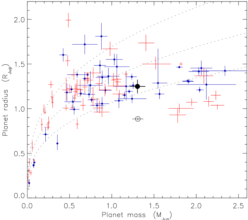
The final physical properties of CoRoT-13 (Table A50) unsurprisingly do not agree well with those of Cabrera et al. (2010). I find radii which are much larger: 26% (3.4$\sigma$) for $R_{\rm A}$ and 41% (4.9$\sigma$) for $R_{\rm b}$. In turn, $g_{\rm b}$ and $\rho_{\rm b}$ are smaller by over a factor of 2. The $\log g_{\rm A}$ also decreases from $4.46\pm 0.05$ to $4.26\pm 0.04$, and the spectroscopically derived $\log g$ for the host star ($4.30\pm 0.10$) is in slightly better agreement with my value. A comparison of the different results for CoRoT-13 b in the context of other TEPs is given in Fig. 18 and shows that my results put it in a region of parameter space occupied by many other TEPs whereas the Cabrera et al. (2010) results make it unusually dense. An improved light curve for the system is urgently needed to verify the revised parameters that I find for the system.

6.14 CoRoT-14

Figure 19: The CoRoT 32 s (upper) and 512 s (lower) light curves of CoRoT-14. Other comments are the same as Fig. 5.

Discovered by Tingley et al. (2011), CoRoT-14 contains a very hot Jupiter ($T_{\rm eq}^{\,\prime}=1936$ K) on a short-period orbit around an F9 V star. The planet’s large mass ($M_{\rm b}=7.7$$\,{\rm M}_{\rm Jup}$) is unusual and is second only to WASP-18 (Hellier et al., 2009a; Southworth et al., 2009c) for objects with $P_{\rm orb}<2$ d. It is rather faint ($V=16.0$) so the light curve is quite scattered, but the RVs are quite sufficient due to its large mass.

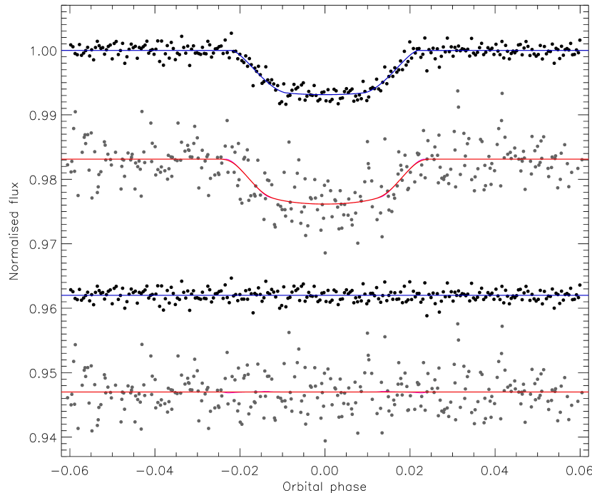
The 32 s data total 217 262 points and 26 279 of these cover 60 transits; after 4$\sigma$-clipping 49 points and phase-binning by a factor of 100 I obtained 263 normal points. The 512 s data comprise 2400 points of which 291 are near transit. One of the 14 transits was rejected due to partial coverage. The remaining 512 s data were modelling using $N_{\rm int}=3$. A third light of $L_{3}=0.07\pm 0.005$ (Tingley et al., 2011) was taken into account.

The best fits are shown in Fig. 19 and tabulated in Tables A51 and A52; correlated noise is unimportant. The LD-fit/fix solutions of the 32 s data are good, but only the LD-fixed solutions are reliable for the 512 s data. The two light curve solutions agree well with each other (Table A53) and with Tingley et al. (2011), as do the resulting physical properties (Table A54). Improved photometry and spectroscopy would be beneficial.

6.15 CoRoT-15

Figure 20: The 512 s light curve of CoRoT-15. See Fig. 5 for details.

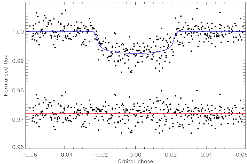
The CoRoT-15 system contains a transiting brown dwarf (Bouchy et al., 2011) with a mass (65$\,{\rm M}_{\rm Jup}$) very similar to those of WASP-30 b (61$\,{\rm M}_{\rm Jup}$; Anderson et al. 2011b) and LHS 6343 Ab (63$\,{\rm M}_{\rm Jup}$; Sect. 6.27). CoRoT-15 is the most difficult to study because of its faintness ($V=15.5$). The CoRoT light curve lasts only 31.7 d and covers ten transits at 512 s cadence. Of the 395 datapoints near transit, four are rejected by a 3$\sigma$ cut and the rest are modelled using $N_{\rm int}=3$ and $L_{3}=0.019\pm 0.003$ (Bouchy et al., 2011).

The jtkebop solutions point to a central transit, and therefore asymmetric errorbars. The LD-fixed and LD-fit/fix solutions agree well (LD-fitted solutions were not tried) so the latter are adopted. Unusually for the CoRoT data, correlated noise was found to be important, with the residual-permutation errorbars slightly larger than the Monte-Carlo ones. The best fit is in Fig. 20 and the model details are in Table A55. My photometric parameters (Table A56) are concordant with those of Bouchy et al. (2011). I find a similarly good match for the physical properties of CoRoT-15 (Table A57), which could be improved by further observations of all relevant types.

6.16 HAT-P-4

Figure 21: Phased light curves of HAT-P-4 compared to the best fits found using jktebop and the quadratic LD law. The transit light curves are, from top to bottom, $z$-band from Kovács et al. (2007), FLWO $i$-band from Winn et al. (2011), FTN $i$-band from Winn et al. (2011), and the EPOCH dataset from Christiansen et al. (2011). The residuals are plotted at the base of the figure, offset from zero.

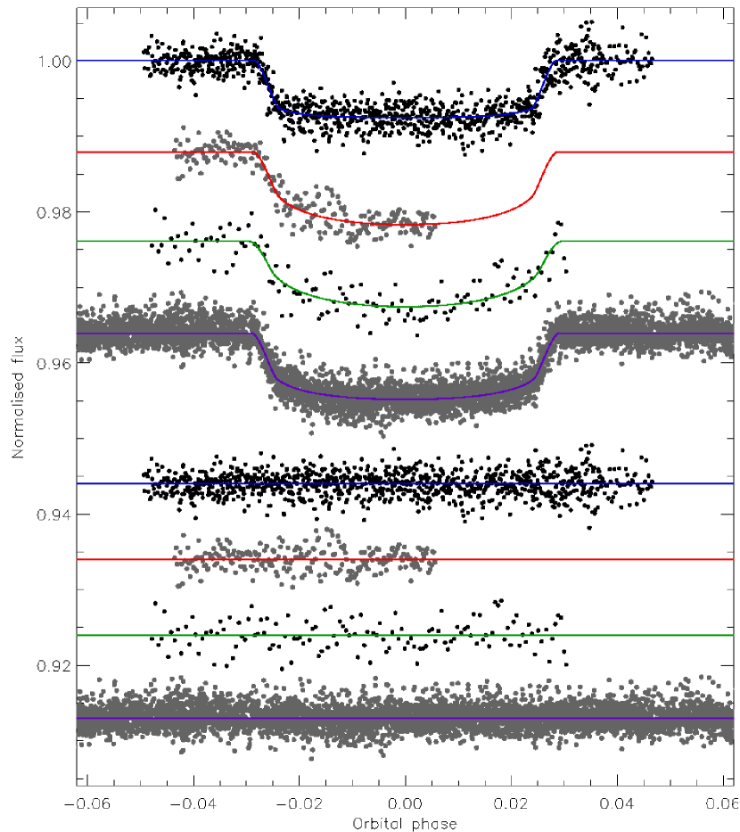
We now leave the CoRoT objects behind and turn to a TEP system with a light curve from the EPOCH project performed by the NASA Deep Impact satellite (Christiansen et al., 2011). HAT-P-4 was discovered by Kovács et al. (2007) to be a low-density TEP orbiting a metal-rich late-F star. Kovács et al. obtained follow-up photometry using the FLWO 1.2 m telescope and KeplerCam, which was subsequently reanalysed by Torres et al. (2008). Further light curves were collected by Winn et al. (2011), who also presented RV observations consistent with alignment of the planetary orbital and stellar rotational axes. Christiansen et al. (2011) analysed the EPOCH data, which cover seven consecutive transits followed by three more taken five months later.

The light curve from Kovács et al. (2007) contains 985 datapoints spread over two transits, whose uncertainties I have multiplied by 1.67 to get $\chi_{\nu}^{\,2}\approx 1$. The LD-fit/fix solutions are clearly better than LD-fixed (larger residuals) and LD-fitted (unphysical LDCs). Correlated noise is slightly important. The parameters are given in Table A58 and the best fit is shown in Fig. 21.

Winn et al. (2011) observed two transits in the $i$-band, a full one with FTN and a partial one with KeplerCam. I binned the 662 points in the first dataset by a factor of 5 to get 133 normal points. The second dataset was modelled using constraints on the time of transit midpoint (Southworth et al., 2007a). In both cases LD-fitted solutions were not attempted (Tables A59 and A60).

I rejected one of the EPOCH transits due to insufficient observational coverage. Of the 6704 points near the other transits, 68 were lost to a 4$\sigma$ clip. The data contain substantial correlated noise due to pointing wander, so I did not phase-bin them. The residual-permutation errorbars are indeed 50% larger than the Monte-Carlo ones. Table A61 shows the results, of which the LD-fit/fix were adopted.

The four final light curve solutions are in good agreement ($\chi_{\nu}^{\,2}<0.04$) except for $k$ ($\chi_{\nu}^{\,2}=1.3$), and were combined by multiplying their probability density functions to get final photometric parameters (Table A62). These are comparatively imprecise because the transit is central, and accord well with literature results.

The jktabsdim results show a significant systematic error from different theoretical model sets, but the final results are reasonable and agree with literature values (Table A63). HAT-P-4 would benefit from a better light curve.

6.17 HAT-P-7

Figure 22: Phased light curves of HAT-P-7 from the Kepler satellite (upper), Winn et al. (2009a) (middle) and EPOCH (lower) compared to the best fits found using jktebop and the quadratic LD law. The residuals are plotted at the base of the figure, offset from zero.

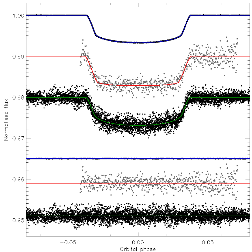
Discovered by Pál et al. (2008), HAT-P-7 was the second TEP found in the Kepler field. It is a relatively massive planet (1.8$\,{\rm M}_{\rm Jup}$) orbiting a relatively massive star (1.5$\,{\rm M}_{\odot}$), and was the second planet found to have a retrograde orbit from RM observations (Winn et al., 2009a) after WASP-17 (Anderson et al., 2010). Kepler has been observing it at short cadence since the start of the mission, and here I have analysed the public data from Q0, Q1 and Q2. These data have already been used to establish the optical phase curve of the planet (Borucki et al., 2009) and the ellipsoidal effect of the star (Welsh et al., 2010). The Kepler data have also be subjected to an asteroseismic investigation by Christensen-Dalsgaard et al. (2010), who used the oscillation spectrum of the data to determine $\rho_{\rm A}$ to high precision. This constraint was not made use of in the current analysis, in order to retain homogeneity of approach. The follow-up light curve from the discovery paper covers only part of the transit and cannot compete with the Kepler data, so was not modelled here.

The Kepler observations are stunning (Fig. 22) and cover 59 transits (five in Q0, 15 in Q1, 39 in Q2). 37 611 of the 186 786 original datapoints are near a transit, of which 55 were rejected by a 4$\sigma$ clip and the rest were phase-binned by a factor of 50 to get 753 normal points. The LD-fitted solutions are good (Table A64) and show that both LDCs need to be fitted to account for data with this level of precision, although correlated noise is formally important.

In order to provide a consistency check on the Kepler data I have also modelled the $i$-band observations of one transit (Table A65) by Winn et al. (2009a) and the EPOCH space-based light curve (Table A66) presented by Christiansen et al. (2010). Whilst the latter again have substantial red noise, they agree well with the Kepler data and the two solutions are therefore combined to obtain the final photometric parameters. The level of agreement with the results of Welsh et al. (2010) is not as good as expected (Table A67). Despite this, HAT-P-7 is one of the best-measured TEP systems, alongside HD 209458 (Paper I) and TrES-2 (Sect. 6.28).

The resulting physical properties are contained in Table A68 and are highly unusual in that the radii of the star and planet are measured to precisions approaching 1%. The agreement with literature results is good overall but with one caveat. Christensen-Dalsgaard et al. (2010) obtained a measurement of $\rho_{\rm A}=0.1926\pm 0.0023$$\,\rho_{\odot}$ by analysing the oscillation spectrum of HAT-P-7 A, which is 2.9$\sigma$ adrift from my transit-derived value of $\rho_{\rm A}=0.2023\pm 0.0024$$\,\rho_{\odot}$. This discrepancy may either gradually sort itself out as additional data appear from Kepler, or alternatively might signal the need to include more sophisticated physics in one or both of the analysis methods.

6.18 HAT-P-11

Figure 23: Individual transits of HAT-P-11 as seen by Kepler. Successive transits are offset by $-$0.03 flux units for clarity.

Figure 24: Phased light curves of HAT-P-11 from the Kepler satellite (upper) and in the $z$-band (lower) from Bakos et al. (2010). See Fig. 22 for further details.

The third TEP discovered in the Kepler field (Bakos et al., 2010) is a low-mass planet (0.084$\,{\rm M}_{\rm Jup}$) in an eccentric orbit around a low-mass star (0.81$\,{\rm M}_{\odot}$). It has been found to have a very oblique orbit through RM observations (Winn et al., 2010; Hirano et al., 2011). Kepler has observed it in short cadence from the start of the mission. As with HAT-P-7 above, Christensen-Dalsgaard et al. (2010) analysed the Q0 and Q1 data and measured a $\rho_{\rm A}$ value which has a very a high precision but an undetermined accuracy.

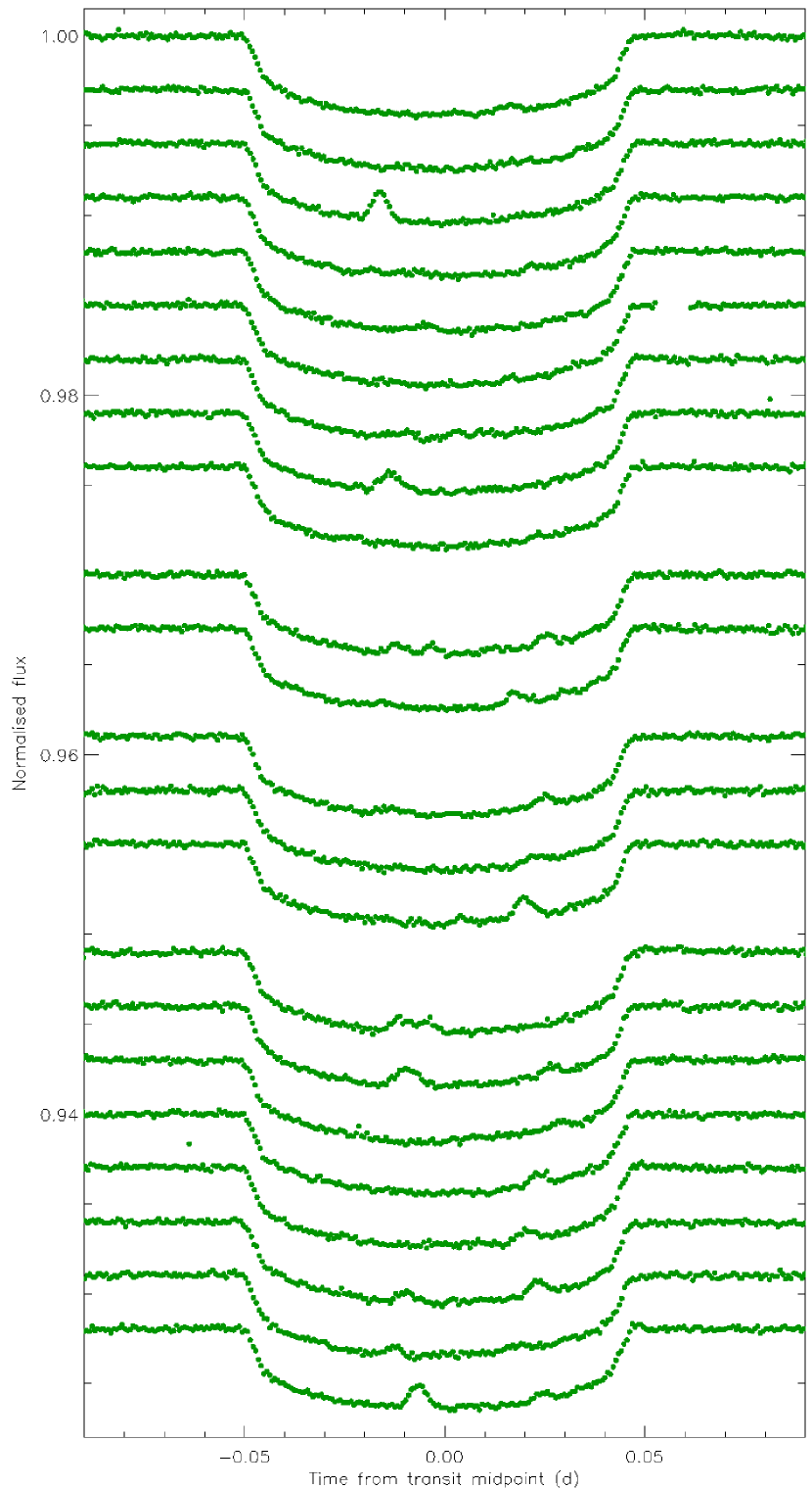
Analysis of the Kepler data is not straightforward, because there is clear evidence of spot activity on the star. Of the 25 transits observed (three in Q0, six in Q1 and 16 in Q2), many are marvellous examples of the phenomenon of a planet transiting a starspot or starspot complex and all are affected to some degree (see Fig. 23). The ratio of the planetary orbital to stellar spin periods is close to 6.0, so every sixth transit will cross over nearly the same part of the stellar surface and thus be similarly affected by spots which evolve on a timescale of 29 d or less, a situation that was predicted by Winn et al. (2010). Fig. 23 certainly shows that there are two preferred orbital phases for spot activity in the Kepler data. A detailed analysis of the spot characteristics will be very interesting.

In the current work I model the Kepler data using my usual approach. The effects of the starspot will therefore be treated as correlated noise. The oblique orbit of HAT-P-11 b means that it transits, at some point, a much greater fraction of the stellar surface than an aligned system would, and with a wide distribution of latitudes. The assumption that the transited parts of the stellar surface on average behave the same as the non-transited areas is therefore more justifiable than in cases such as CoRoT-2. Due to LD, the effects of starspots are much stronger near the centre of the star than its limb (e.g. Sanchis-Ojeda et al., 2011). In contrast, starspot deviations have the greatest effect on a photometric model when they occur at the partial phases of the transit. Treating them as correlated noise is therefore more likely to lead to an overestimate rather than an underestimate of the errorbars.

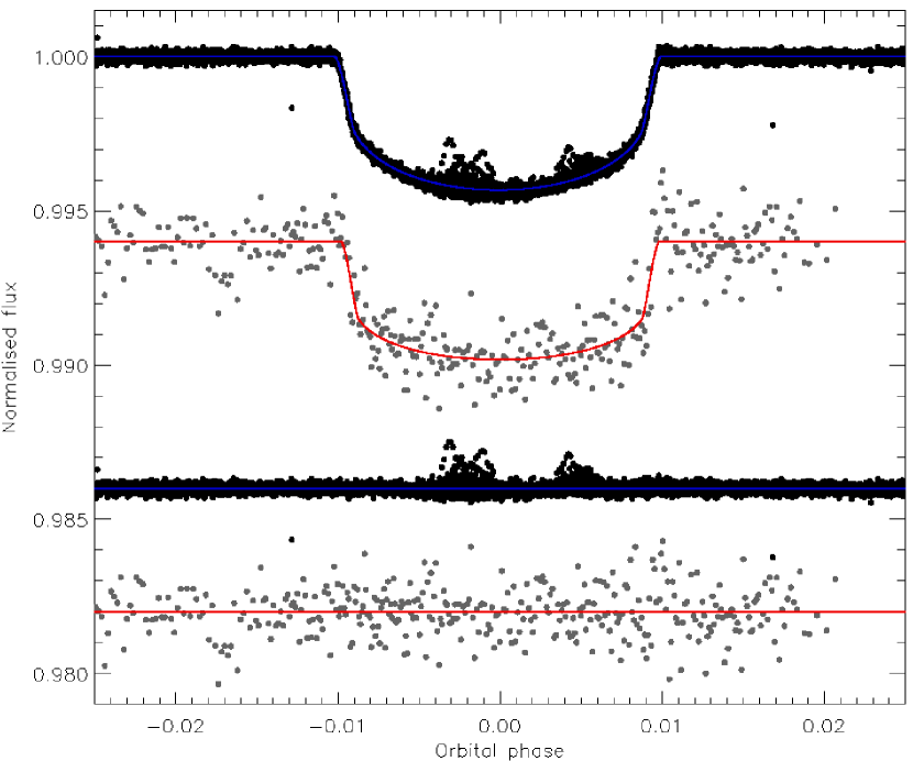
The Kepler Q0 to Q2 data comprise 186 802 datapoints of which 12 535 are adjacent to a transit. They were not phase-binned, as this might affect the estimation of the starspot-induced correlated residuals of the fit. The Kepler data don’t agree exactly with previous orbital ephemerides of the system so the $T_{0}$ from Bakos et al. (2010) was included as a constraint following the approach of Southworth et al. (2007a). I also accounted for orbital eccentricity using $e\cos\omega=0.261\pm 0.082$ and $e\sin\omega=0.085\pm 0.043$ (Winn et al., 2010). The LD-fitted solutions are poor and have unphysical LDCs so the LD-fit/fix solutions were preferred (Table A69). The residual-permutation errors were larger than the Monte Carlo ones for the inclination but not for the other photometric parameters, supporting the approach taken to fit the data. The best fit is in Fig. 24.

Additional light curves are available from Bakos et al. (2010), comprising eight transits observed in the $z$-band using KeplerCam, one in the $r$-band with the same instrument, and three in the $I$-band with the Konkoly Schmidt. The first of these datasets is worth solving as a check of the Kepler data: the 4110 datapoints were phase-binned by a factor of ten to obtain 410 normal points. Correlated noise was not found to be important, and the LD-fit/fix solutions were adopted (Table A70). The agreement with the Kepler data is good (Table A71). Literature results are in moderate agreement, but the current results are to be preferred as they are the first to be based on the Kepler observations.

The jktabsdim results suggest that the measured $T_{\rm eff}$ of the host star is quite high ($4780\pm 50$ K), causing the system to occupy the zero-age edge of the model grids. A hefty decrease of 300 K in $T_{\rm eff}$ would be needed to assuage this problem, and would shift $M_{\rm A}$ from 0.82 to 0.75$\,{\rm M}_{\odot}$ with other parameters less strongly affected. I therefore acquired some alternative $T_{\rm eff}$ estimates from a number of sources. The Tycho $B-V$ value (Høg et al., 1997) supplemented by the calibration of Sousa et al. (2008) returns $T_{\rm eff}=4852$ K. $B-V$ is not generally regarded as a good $T_{\rm eff}$ indicator for late-type dwarfs: the same value for this colour index equates to a K5 star with $T_{\rm eff}=4410$ K using the tables of Zombeck (1990). Using the 2MASS $JHK_{s}$ (Skrutskie et al., 2006) magnitudes is a better bet: the $V-K_{s}$ colour index and the calibration of Casagrande et al. (2008) yields $T_{\rm eff}=4765$ K. Dr. B. Smalley has kindly calculated the luminosity of HAT-P-11 A from the available broad-band optical and infrared photometry and the Hipparcos parallax (Perryman et al., 1997) to be $\log(L/\,{\rm L}_{\odot})=-0.61$. This agrees with the jktabsdim solutions for the measured $T_{\rm eff}$ of the star ($-0.63$) but not with those for the lower $T_{\rm eff}$ ($-0.77$). The $T_{\rm eff}$ measurement from Bakos et al. (2010) is supported by the investigations above.

Table A72 shows my calculated physical properties for HAT-P-11 b compared to literature solutions. Bakos et al. (2010) find smaller radii for the two components which may be down to differences in analysis. In the HAT methodology the stellar parameters are forced to agree with a theoretical stellar model (usually interpolated from the Y² isochrones); in my solution process I find the point of closest agreement but do not require this to exactly reproduce a point in a grid of theoretical predictions. I find a very young but poorly constrained age, which is in accordance with the starspot activity seen in both the Kepler and the HAT data. Christensen-Dalsgaard et al. (2010) derived $\rho_{\rm A}=1.7846\pm 0.0006$$\,\rho_{\odot}$ (errorbar does not account for systematic errors) from the oscillation spectrum of HAT-P-11 A in the Kepler light curve. This indicates a much less dense star than I find ($2.415\pm 0.097$$\,\rho_{\odot}$), a similar situation to HAT-P-7 but with a much stronger discrepancy. Further investigation is needed to understand the disagreement; extra RV measurements would be useful to refine the $K_{\rm A}$, $e\cos\omega$ and $e\sin\omega$ values.

6.19 HD 17156

Figure 25: The light curves of HD 17156 compared to the jktebop best fit. Top is HST/FGS, middle and bottom are $(b+y)/2$ and $z$ from Winn et al. (2009c). See Fig. 22 for further details.

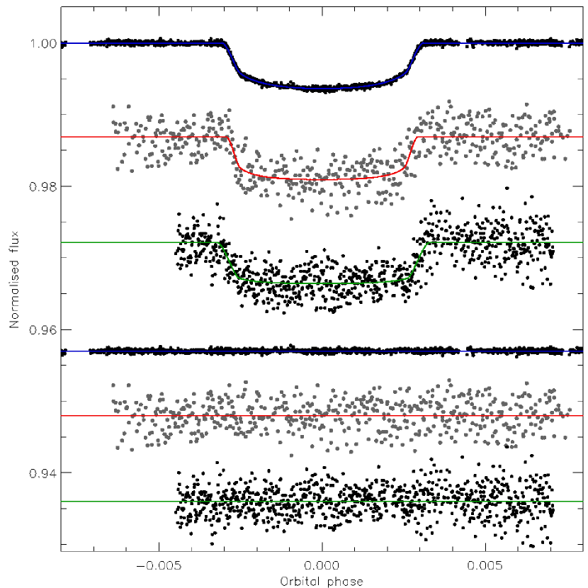
The planet orbiting HD 17156 was discovered by the RV method by Fischer et al. (2007), who also searched for transits but did not detect them or rule out their existence. A transit was soon observed using three telescopes by Barbieri et al. (2007), as part of the transitsearch.org network (Seagroves et al., 2003). Further transit light curves were obtained by Gillon et al. (2008), Barbieri et al. (2009) and Irwin et al. (2008). Two good light curves were presented by Winn et al. (2009c), covering the transit on Christmas Day in 2007. The RM effect has been observed on multiple occasions (Narita et al., 2008; Cochran et al., 2008; Barbieri et al., 2009; Narita et al., 2009) and overall indicates axial alignment.

An extensive analysis of HD 17156 was performed by Nutzman et al. (2011) and Gilliland et al. (2011) based on data obtained using the HST/FGS. The asteroseismic study (Gilliland et al., 2011) yielded a mean density and age for the star. The theoretical uncertainty of the former quantity is probably small, but is significant for the latter quantity. The HST/FGS data cover three transits, which were used by Nutzman et al. (2011) to measure the physical properties of the system. Analyses including the asteroseismic $\rho_{\rm A}$ as a constraint are in good agreement with standard analyses, but with smaller errorbars (by a factor of three for $R_{\rm A}$ and $R_{\rm b}$). I did not include the asteroseismic constraint in my analysis, in order to retain homogeneity with the results for other systems.

I have solved the two light curves from Winn et al. (2009c), which are in the $(b+y)/2$ and $z$ passbands, each covering one transit. I also modelled the HST data from Nutzman et al. (2011), which comprises partial coverage of each of three transits, using a light curve which has been corrected for instrumental effects. The FGS data were taken with the F583W filter which covers 440–710 nm, so I adopted for LDCs appropriate for a combined $g$+$r$ filter. The orbital shape of HD 17156 was accounted for by adopting $e=0.6768\pm 0.0304$ and $\omega=121.71\pm 0.43$ deg (Nutzman et al., 2011). The best fits are exhibited in Fig. 25.

The results for the HST light curve are given in Table A73 and LD-fit/fix is the best alternative. Correlated noise is marginally important. The $(b+y)/2$ data prefer a higher $i$ and thus smaller $r_{\rm A}$ and $r_{\rm b}$ (Table A74), whereas the $z$ observations yield the opposite situation (Table A75). The two datasets agree with the HST results overall, so the HST ones are adopted as the final parameters (Table A76). Their agreement with published values is reasonable.

The physical properties of HD 17156 are shown in Table A77 and reveal some model-dependent error which stems primarily from the DSEP models. The agreement with literature values is again good, and I provide the first measurement of $T_{\rm eq}^{\,\prime}$ and $\Theta$. HD 17156 is a well-characterised system which is not in need of further observations.

6.20 HD 80606

Figure 26: The Spitzer light curve of HD 80606 (Hébrard et al., 2010). See Fig. 22 for further details.

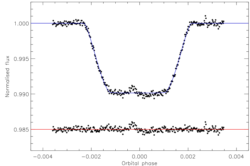
HD 80606 b was found to be a planetary-mass object with a period of 111.8 d by Naef et al. (2001) from extensive RV observations. At the time of discovery it was the most eccentric exoplanet known ($e=0.927$). Laughlin et al. (2009) observed an occultation of the planet whilst using Spitzer to probe the heating of the planet around periastron. Based on the parameters then known, Laughlin et al. calculated a probability of 15% that a transit also occurs, and encouraged follow-up observations to detect it. The system was monitored over the next predicted time of transit and duly found to be a TEP by Moutou et al. (2009), Garcia-Melendo & McCullough (2009) and Fossey et al. (2009).

RM observations of HD 80606 have been obtained and studied by Moutou et al. (2009), Pont et al. (2009), Hébrard et al. (2010) and Winn et al. (2009b), with a good agreement that the orbit is oblique to high confidence. Coupled with the high eccentricity, this has bearing on its formation and evolution mechanisms (Naef et al., 2001; Mardling & Lin, 2002; Matsuo et al., 2007). The relatively high mass of the planet (4.11$\,{\rm M}_{\rm Jup}$) agrees with the established pattern that TEPs in eccentric orbits are generally the massive ones (Southworth et al., 2009c).

Spectral synthesis analyses of the parent star have been performed by Naef et al. (2001), Santos et al. (2004) and Gonzalez et al. (2010): I adopt the $T_{\rm eff}$ from Santos et al. (2004) as it is the middle of the three values and its errorbar encompasses the other two; I use the Gonzalez et al. (2010) $\left[\frac{\rm Fe}{\rm H}\right]$ value because all three agree and it has an equitable errorbar. I take the $K_{\rm A}$ value from the most recent detailed RV analysis, Winn et al. (2009b).

Good light curves of HD 80606 are difficult to obtain due to the long transit duration (nearly 12 hours) and orbital period. The transit discovery light curves (Moutou et al., 2009; Garcia-Melendo & McCullough, 2009; Fossey et al., 2009) all missed ingress as it occurred during daylight. Winn et al. (2009b) combined data from eight observing sites spread through mainland USA and Hawaii to obtain full coverage of the 2009 June transit, but the resulting light curve was still a long way from definitive. Shporer et al. (2010) and Hidas et al. (2010) performed similar observing campaigns covering several transits, but the data are unfortunately strongly affected by systematics. Hébrard et al. (2010) used Spitzer to obtain a complete and high-quality light curve of the 2010 January transit in the IRAC 4.5 $\mu$m passband. This is by far the best light curve of any transit of HD 80606, and is the only one analysed here.

The Spitzer data were binned by a factor of 100 to lower the number of datapoints from 31 767 to 318. The resulting time resolution is 215 s, which is reasonable for such a long-duration transit. A disturbance near mid-eclipse is noticable and can be attributed to starspots (Fig. 26); this was treated as correlated noise in the jktebop analysis (see Sect. 6.18). The flux from the planet in this near-infrared passband must be accounted for, which was done by including a light ratio of $0.001\pm 0.001$ with the method described by Southworth et al. (2007a). This light ratio gives a secondary eclipse of similar depth to that observed by Laughlin et al. (2009), with a conservative errorbar to allow for inefficient energy redistribution within the planetary atmosphere. The orbital shape was accounted for using $e\cos\omega=0.4774\pm 0.0018$ and $e\sin\omega=-0.8016\pm 0.0017$ (Hébrard et al., 2010). The LD-fitted solutions yield unphysical LDCs so the LD-fit/fix solution was adopted (Table A78). Correlated noise is important, due to the treatment of the starspot. The final photometric parameters (Table A79) are in reasonable agreement with published values.

The jktabsdim results show that the systematic error (model disagreement) is relatively high, and dominates the error budget for $M_{\rm A}$, $M_{\rm b}$ and $a$ (Table A80). The solution with the dEB constraint is also somewhat different to the solutions using theoretical models. The source of these problems is not obvious, but the discrepancies are small enough that HD 80606 is one of the best-characterised TEP systems.

6.21 Kepler-4

Figure 27: Phased long-cadence (top) and short-cadence (second from top) light curves of Kepler-4 compared to the best fit found using jktebop and the quadratic LD law. For the long-cadence data the fit is shown by a blue line, and an evaluation of the same model but without numerical integration is shown by a purple line. The residuals are plotted at the base of the figure, offset from unity. The purple line through the residuals shows the difference between the fit to the data and an evaluation of the same model but without numerical integration.

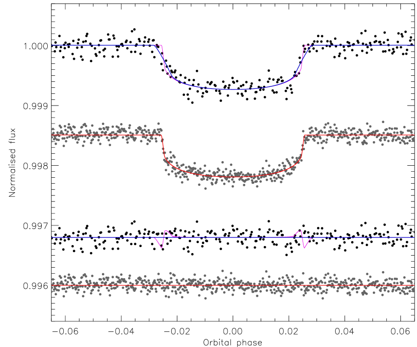
Kepler-4 was the first TEP system to be announced as a discovery of the Kepler satellite (Borucki et al., 2010a) and is a very low-mass object (0.075$\,{\rm M}_{\rm Jup}$) orbiting a slightly evolved star ($\log g=4.17$). It has also been studied by Kipping & Bakos (2011b). Eccentricity is significant at only 2$\sigma$ and additional RV measurements are necessary to investigate this further. The available Kepler data cover 13 shallow transits at long cadence (29.4 min) in Q0 and Q1 and 26 transits at short cadence (58.8 s) in Q2.

The addition of Q2 data over Q0 and Q1 allows an improvement of the orbital ephemeris. The short-cadence data were binned to the time resolution of the long-cadence data. The long-cadence and binned short-cadence data were then modelled using jktebop and $N_{\rm int}=10$ to find:

$$T_{0}={\rm HJD}\,\,2\,454\,956.61132(92)\,+\,3.213658(38)\times E$$

where the bracketed quantities give the uncertainties in the preceding digit, and the uncertainties come from 100 MC simulations.

The long-cadence transit data were cut from the full light curve and normalised as described in Sect. 5, giving 323 datapoints out of the original 2101. The 123 536 short-cadence observations were treated similarly, then phase-binned by a factor of 25 to yield 708 normal points. I assumed a circular orbit and a third light of $L_{3}=0.02\pm 0.02$. The long-cadence data do not constrain the fit well; parameter perturbations could not be applied in the Monte Carlo analysis so these errorbars may be optimistic. The long-cadence data were solved using $N_{\rm int}=10$ (Table A81) and the short-cadence data were solved without using numerical integration (Table A82). The best fits are given in Fig. 27. In both cases the LD-fit/fix solutions were best. The residual-permutation errorbars were much larger than the Monte-Carlo ones for the long-cadence light curve, which is likely due to the inability to apply parameter perturbations in this case.

The solutions for the two datasets agree well and were combined by multiplying their probability density functions to give final photometric parameters (Table A83). The photometic parameters from Kipping & Bakos (2011b) disagree with those from Borucki et al. (2010a): the latter find a lower inclination and thus larger $r_{\rm A}$ and $r_{\rm b}$. My results support those of Borucki et al. (2010a) and I am unable to completely reproduce the Kipping & Bakos (2011b) results by modifying my treatment of eccentricity or numerical integration.

The physical properties of Kepler-4 (Table A84) show a reasonable agreement with literature results albeit with substantially larger errorbars in some cases. This is despite the availability of much more extensive (and higher-cadence) observations available for my analysis. The Kepler satellite continues to observe the system at short cadence so a much improved light curve will gradually accumulate. Additional spectroscopy to improve the $T_{\rm eff}$ and $K_{\rm A}$ measurements should be a high priority.

6.22 Kepler-5

Figure 28: Phased light curves of Kepler-5. See Fig. 27 for further details.

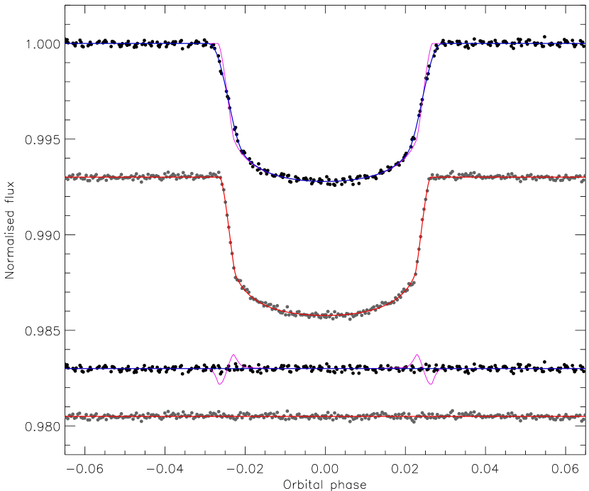
The discovery of Kepler-5 was announced by Koch et al. (2010): the planet is relatively massive (2.04$\,{\rm M}_{\rm Jup}$) and the star is quite evolved ($\log g=4.17$). It has also been studied by Kipping & Bakos (2011b). The available Kepler data now comprise 12 transits studied at long cadence during Q0 and Q1, of which 330 of the 2101 datapoints occur near to a transit, and 23 transits at short cadence after rejection of one transit due to systematic noise. The 123 536 short-cadence datapoints were reduced into 379 normal points. A revised orbital ephemeris was measured from the Q0, Q1 and Q2 data:

$$T_{0}={\rm HJD}\,\,2\,454\,955.90059(36)\,+\,3.548469(15)\times E$$

using the same approach as for Kepler-4.

A third light of $L_{3}=0.02\pm 0.002$ and a circular orbit were assumed (Koch et al., 2010) and the long-cadence data were modelled using $N_{\rm int}=10$. The jktebop solutions (Tables A85 and A86) show that correlated noise is unimportant and that the LD-fitted results are viable. Agreement between the two datasets is not good and can be attributed to information loss at the long cadence. I therefore adopt the short-cadence solutions as final (Table A87). I find a notably smaller $r_{\rm A}$ and $r_{\rm b}$ than Koch et al. (2010) and Kipping & Bakos (2011b), which reflects the difference between the long-cadence data (which were available for those studies) and the better short-cadence observations (which were not). The uncertainties given by Koch et al. (2010) are too low. The best fits are shown in Fig. 28.

The jktabsdim results are contained in Table A88 and expectedly disagree with literature studies based on only the long-cadence data: I find smaller masses and radii for both star and planet. The discovery paper (Koch et al., 2010) obtained two solutions corresponding to different evolutionary stages for the host star (with masses 1.21 and 1.38 $\,{\rm M}_{\odot}$), and endorsed the more evolved alternative. I do not find this problem, due to my refined photometric parameters. Additional photometric observations are needed, are currently being obtained by the satellite, and will make Kepler-5 one of the best-charaterised TEP systems.

6.23 Kepler-6

Figure 29: Phased light curves of Kepler-6. See Fig. 27 for further details.

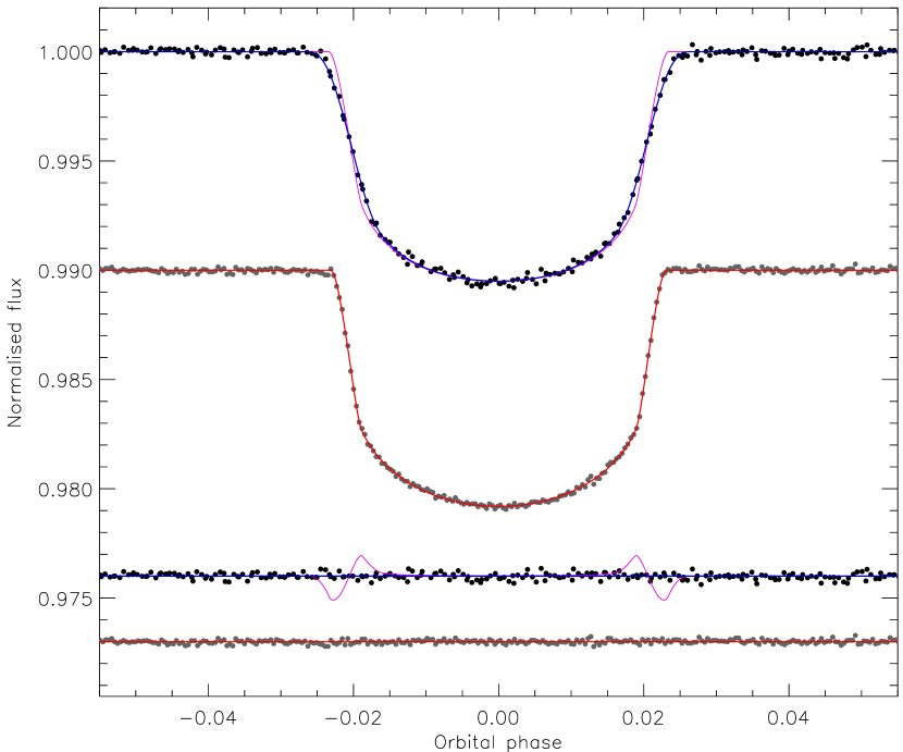
Kepler-6 was found to be a TEP by Dunham et al. (2010) and is interesting because of the high metallicity of the host star ($\left[\frac{\rm Fe}{\rm H}\right]=0.34\pm 0.05$). The same long-cadence data were studied by Kipping & Bakos (2011b), who found a solution with a higher orbital inclination and 2.6$\sigma$ signficant signal in the TTV peridogram which may indicate stellar activity. The Kepler Q0 and Q1 data cover 13 transits at long cadence, whereas the Q2 data include 41 transits at short cadence. A new orbital ephemeris was determined from these data:

$$T_{0}={\rm HJD}\,\,2\,454\,954.485805(64)\,+\,3.2347020(33)\times E$$

The long cadence data comprise 2102 points of which 246 are near a transit. These were modelled using $N_{\rm int}=10$ to yield the results in Table A89. The solutions are very sensitive to the treatment of LD: LD-fixed gives a poor internal agreement and LD-fitted returns unphysical LDCs, so the LD-fit/fix results were adopted. The 123 536 short-cadence datapoints were reduced into 34 normal points and the LD-fit/fix solutions were best (Table A90). In both cases $L_{3}=0.033\pm 0.004$ (Dunham et al., 2010) was incorporated and correlated noise was found to be inconsequential. The two datasets agree well so the parameters were combined (Table A91). Published studies agree well with my results, although their errorbars are questionable. The best fits are shown in Fig. 29.

The physical properties of Kepler-6 are given in Table A92. The DSEP model solutions disagree with the others so are not included in the final results. I find a somewhat smaller planet and star compared to Dunham et al. (2010), whereas Kipping & Bakos (2011b) agree with my results within the errors. Kepler continues to observe Kepler-6 at short cadence and additional RV measurements would also be useful.

6.24 Kepler-7

Figure 30: Phased long-cadence light curve of Kepler-7. See Fig. 27 for further details.

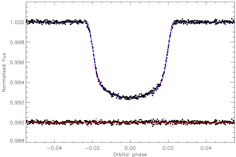
Discovered by Latham et al. (2010), this a very low-density TEP (0.10$\,\rho_{\rm Jup}$) around a slightly evolved star ($\log g=3.96$). The same data were also studied by Kipping & Bakos (2011b), who detected an occultation with a significance level of 3.5$\sigma$. The Q2 data are long-cadence, so no short-cadence data are available for analysis. The Q0, Q1 and Q2 observations cover 26 transits, and 947 of the 6177 datapoints were retained for the jktebop analysis. $L_{3}=0.025\pm 0.005$, a circular orbit and $N_{\rm int}=10$ were adopted. The updated orbital ephemeris is:

$$T_{0}={\rm HJD}\,\,2\,454\,967.27598(11)\,+\,4.8854948(82)\times E$$

The LD-fitted results are reliable and have reduced residuals compared to the LD-fit/fix solutions (Table A93). Correlated noise is insignificant. I find a lower inclination and therefore a higher $r_{\rm A}$ and $r_{\rm b}$ than previous studies (Table A94), and investigations reveal that this is primarily due to inclusion of the Q2 data. The best fits are shown in Fig. 30.

The physical properties of Kepler-7 (Table A95) reveal that the star is one of the most evolved known to host a TEP, and the planet itself is the second-most rarefied known after WASP-17 (Anderson et al., 2010, 2011a). As expected from the photometric parameters, my physical properties do not agree well with those previously published. Confirmation of this will be possible soon, as Kepler-7 has been observed in short cadence by Kepler from Quarter 3 onwards. New RV measurements would also be worthwhile.

6.25 Kepler-8

Figure 31: Phased light curves of Kepler-8. See Fig. 27 for further details.

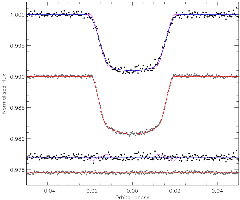
Like Kepler-7, Kepler-8 is a low-density TEP (0.21$\,\rho_{\rm Jup}$) orbiting a slightly evolved star ($\log g=4.18$). Jenkins et al. (2010a) and Kipping & Bakos (2011b) have studied the Kepler Q0 and Q1 long-cadence data, whereas the Q2 short-cadence observations are now available. A refined orbital ephemeris was established as:

$$T_{0}={\rm HJD}\,\,2\,454\,954.11844(18)\,+\,3.5225047(76)\times E$$

The long-cadence observations cover 13 transits, and I retain 265 of the original 2098 datapoints (solved using $N_{\rm int}=10$). The Q2 data consist of 123 536 points covering 24 transits, which I phase-binned down to 299 normal points. The third light value given by Jenkins et al. (2010a) does not have an errorbar, so I adopt $L_{3}=0.0075\pm 0.0075$ to be conservative. The best fits can be seen in Fig. 31. Models of the long-cadence data are rather sensitive to the treatment of LD and are also in comparatively poor agreement with the short-cadence models (Tables A96 and A97). I therefore adopt the LD-fit/fix flavour of the latter (Table  A98), which is also in accord with and more precise than literature studies. The errorbars found by Jenkins et al. (2010a) are smaller than expected.

The absolute dimensions of Kepler-8 (Table A99) agree well with published values and establish it as a well-understood system. Kepler continues to observe Kepler-8 photometrically and further RV observations are merited.

6.26 KOI-428

Figure 32: Phased light curve of KOI-428. See Fig. 27 for further details.

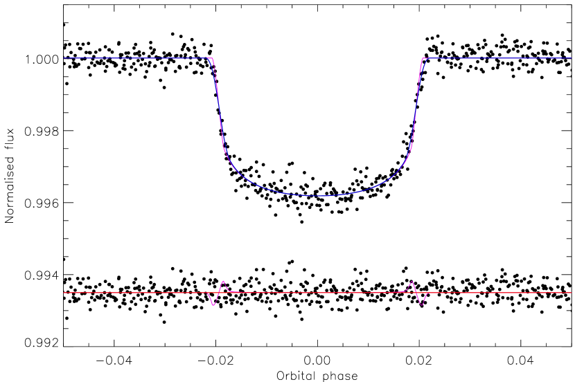
KOI-428 was one of the 306 Kepler Objects of Interest that was presented to the astronomical community by Borucki et al. (2011); the 400 brightest ones were retained for in-house analysis by the Kepler Team. Follow-up spectroscopic observations by Santerne et al. (2011) have subsequently shown this to be a system containing a relatively massive planet (2.1$\,{\rm M}_{\rm Jup}$) orbiting a comparatively hot star (6510 K).

The Kepler Q1 and Q2 data contain 12 transits observed at long cadence, compared to only four in the Q1 data available to Santerne et al. (2011). 741 of the 5708 datapoints were retained; one of the 12 transits was rejected because it is deformed by instrumental artefacts arising from a pointing jump. These were solved using $N_{\rm int}=10$, a circular orbit and no $L_{3}$ (Table A100). Correlated noise is negligible. I find a lower inclination and thus larger $r_{\rm A}$ and $r_{\rm b}$ compared to Santerne et al. (2011), but the values are within their errorbars (Table A101). Fig. 32 shows the best fit to the light curve. The revised orbital ephemeris is:

$$T_{0}={\rm HJD}\,\,2\,455\,005.51858(50)\,+\,6.873130(75)\times E$$

jktabsdim returns a noticably larger but less massive star compared to Santerne et al. (2011), as expected given the slightly different photometric parameters (Table A102). The model fits prefer a $T_{\rm eff}$ lower by 80 K (0.8$\sigma$), so this may indicate that analysis of the Kepler data in isolation results in a star which is too large. KOI-428 remains on the Kepler target list so additional data will be available soon. The errorbars quoted by Santerne et al. (2011) are too small. Further spectroscopic study of this object is warranted.

6.27 LHS 6343

Figure 33: Phased light curve of LHS 6343. See Fig. 27 for further details.

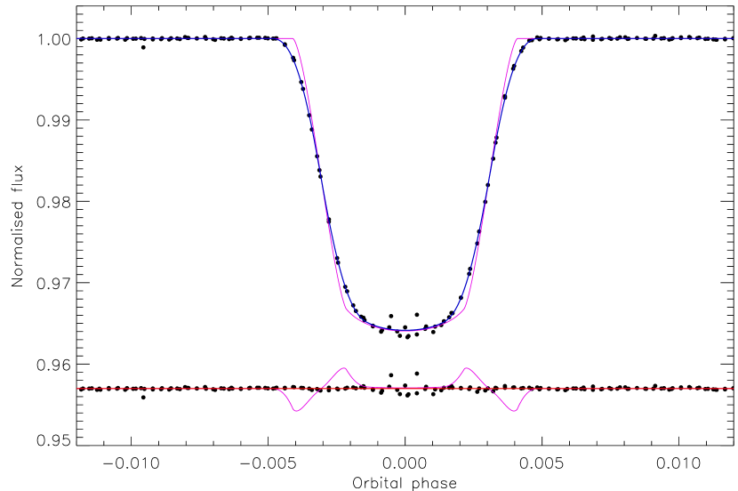
LHS 6343 is a nearby M dwarf (Luyten, 1979) which was found to host a small transiting object by Johnson et al. (2011) based on Kepler data. Follow-up imaging and spectroscopic observations (Johnson et al., 2011) revealed that the system contains two M dwarfs (A and B) separated by 0.55^′′  and that the brighter component A hosts a likely brown-dwarf companion with an orbital period of 12.71 d. The Kepler Q0, Q1 and Q2 data contain a total of 11 transits observed at long cadence.

The Kepler observations are of the combined flux of the three components, and a light ratio of B versus A has not been directly observed. The adaptive-optics imaging obtained by Johnson et al. (2011) give magnitude differences in the $JHK_{s}$ passbands of $0.49\pm 0.05$, $0.49\pm 0.05$ and $0.45\pm 0.05$, respectively. The characteristics of these passbands are such that an extrapolation to the wide Kepler passband is reasonable for stars as similar as A and B. This was performed using the process outlined in Paper III (see also Southworth et al., 2010), resulting in $L_{3}=0.29\pm 0.09$. Measurements of the flux ratio at optical wavelengths would be useful in refining these numbers.

Johnson et al. (2011) obtain $T_{\rm eff}=3130\pm 20$ K for component A from the calculated $V$ and observed $K_{s}$ magnitudes of the star applied to the photometric calibrations of Casagrande et al. (2008). The quoted errorbar is clearly a precision rather than a true uncertainty. I therefore extrapolated the infrared light ratios into the $V$ band to obtain the $V-K_{s}$ colour index which, with the calibrations from Casagrande et al. (2008), gives $T_{\rm eff}=3300\pm 200$ K for component A where the errorbar is conservative. My $T_{\rm eff}$ value was used in the analyses below.

The 6177 long-cadence datapoints from the Kepler Q0, Q1 and Q2 observations were slimmed down to 268 points nearby a transit. These were modelled with jktebop using $L_{3}=0.29\pm 0.09$ (see above), $e=0.056\pm 0.032$, $\omega=337^{\circ}\pm 56^{\circ}$ (Johnson et al., 2011) and $N_{\rm int}=10$. I included $P_{\rm orb}$ and $T_{0}$ as fitted parameters constrained by the $T_{0}$ value found by Johnson et al. (2011) from a ground-based observation of one transit. The ensuing orbital ephemeris is:

$$T_{0}={\rm HJD}\,\,2\,454\,995.358014(44)\,+\,12.7138107(73)\times E$$

The LD-fixed solutions are poor (Table A103). The LD-fit/fix alternatives are better, but the quality of fit is hampered by scattered data mischievously placed right at the transit midpoint. Kepler continues to observe LHS 6343 so an improved light curve is in the pipeline. Correlated noise is not important. Compared to Johnson et al. (2011) I find a smaller $k$ and larger $r_{1}$, as well as larger errorbars despite having many more photometric observations (Table A104). The best fit is in Fig. 33.

Derivation of the physical properties of the star and its substellar transiting companion is difficult due to the low mass of the former object. Theoretical stellar models are unreliable in this regime (see fig. 4 in Paper III) so an additional systematic error should be added to those quoted in Table A105. Compared to Johnson et al. (2011) I find the star to be more massive, which propagates into a correspondingly larger mass for the companion of $M_{\rm b}=70\pm 6$$\,{\rm M}_{\rm Jup}$ close to the stellar/substellar boundary. Further spectroscopic and spatially resolved optical observations would be useful in pinning down the $T_{\rm eff}$ of the host star and the mass of its companion.

6.28 TrES-2

Figure 34: Phased light curves of TrES-2 compared to the best fits found using jktebop and the quadratic LD law. From top to bottom the data are from Kepler, the 790.2 nm then 794.4 nm sets from Colón et al. (2010), $R$-band from Rabus et al. (2009), and EPOCH from Christiansen et al. (2011). See Fig. 26 for further details. See Paper III (sect. 4.7 and fig. 11) of Paper III for previous results.

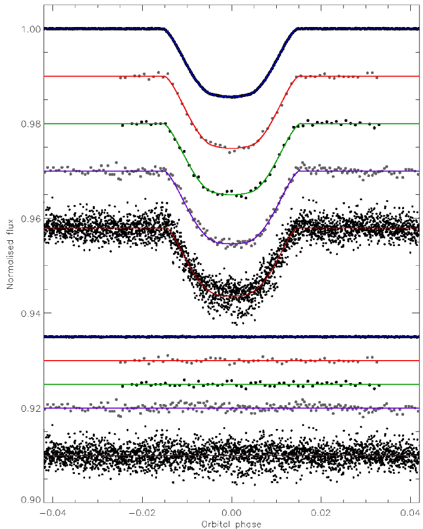
TrES-2 was discovered by the Trans-Atlantic Exoplanet Survey (O’Donovan et al., 2006) and subsequently treated in Paper I and Paper II. TrES-2 was the first TEP discovered in the Kepler field, and a light curve of stunning quality from this satellite is now available (Gilliland et al., 2010). An analysis of these data has been given by Kipping & Bakos (2011a). In addition, excellent ground-based light curves have been obtained by Colón et al. (2010) and it was one of the targets of the EPOCH project using the NASA Deep Impact spacecraft (Christiansen et al., 2011). We also add to this dataset the Johnson $R$-band light curve obtained by Rabus et al. (2009) in the course of a TTV study. The system offers one complication: a fainter star at a separation of 1.09^′′ (Daemgen et al., 2009). TrES-2 was revisited in Paper III to account for this situation.

The Kepler data cover four transits in Q1, 14 in Q1 and 34 in Q2 (ignoring one near an instrumental artefact), all at short cadence. The 186 802 original datapoints were reduced to 18 310 by rejecting observations far from transit, then to 18 297 by a 4$\sigma$ clip, and then to 311 normal points by phase-binning by a factor of 30. $L_{3}=0.0258\pm 0.0008$ was used and the LD-fit/fix solutions adopted (Table A106). Correlated noise was not important. Although Kepler continues to observe TrES-2, it is already the photometrically best-measured TEP known. The light curve fits are shown in Fig. 34, which is best viewed in conjunction with Fig. 11 in Paper III.

The two light curves from Colón et al. (2010) cover the same transit in two very narrow passbands, at 790.2 and 794.4 nm, obtained using the 10.4 m GranTeCan and OSIRIS imager equipped with a tunable filter. $L_{3}=0.0355\pm 0.0005$ was used for both passbands. For the 790.2 nm data the LD-fixed solutions had to be adopted, and correlated noise was found to be moderately important (Table A107). The LD-fit/fix solutions could be adopted for the 794.4 nm data, for which correlated noise was found to be unimportant (Table A108.

The $R$-band data from Rabus et al. (2009) comprise data from five transits which are supplied already phased and binned. I scaled the errorbars by a factor of 0.485 to obtain $\chi_{\nu}^{\,2}\approx 1$ and modelled them using $L_{3}=0.0287\pm 0.0007$. The LD-fit/fix solutions are reasonable (Table A109) and correlated noise is incidental (as expected given the phase-binning process).

The EPOCH data (Christiansen et al., 2011) cover eight transits. 3534 of the original 27 724 datapoints were retained, of which 17 were subsequently rejected by a 3.5$\sigma$ clip. They were not phase-binned as correlated noise was correctly expected to be important. $L_{3}=0.026\pm 0.002$ was assumed. I had to adopt the LD-fixed solutions as the LD-fit/fix and LD-fitted alternatives gave anomalous results and negative LDCs (Table A110).

The overall results for each light curve are given in Table A111 and show an excellent agreement overall. $k$ is as expected the least concordant parameter, but even here the agreement is at the level of $\chi_{\nu}^{\,2}=0.9$. The final photometric parameters are the weighted means of the ones for each light curve. Their agreement with published values is in general excellent except, perplexingly, for those of Kipping & Bakos (2011a) which are the only other ones to be derived from the Kepler data of TrES-2. Similar concerns have been noted for Kepler-4 to Kepler-8, so there may be a small systematic difference in the results from Kipping & Bakos compared to other researchers.

TrES-2 is of particular interest because Mislis & Schmitt (2009) and Mislis et al. (2010) have found evidence for a decrease in the system’s orbital inclination. The Kepler data rule out an effect of the expected size, and do not provide evidence of changes in any of the photometric parameters (see also Kipping & Bakos 2011a). A natural explanation of the previous detection of a change in inclination would be the presence of subtle systematic errors in transit light curves.

The jktabsdim results are given in Table A112 and show that TrES-2 is now very well characterised. The photometric parameters contribute only a small part of the error budget for the measurements of its physical properties. The best way to improve the results further would be to obtain a more precise $\left[\frac{\rm Fe}{\rm H}\right]$ value.

6.29 TrES-3

Figure 35: Phased light curves of TrES-3 compared to the best fits found using jktebop and the quadratic LD law. From top to bottom are the 790.2 nm then 794.4 nm datasets from Colón et al. (2010), and the EPOCH data from Christiansen et al. (2011). See Paper III (sect. 4.8 and fig. 12) for previous results. See Fig. 26 for further details.

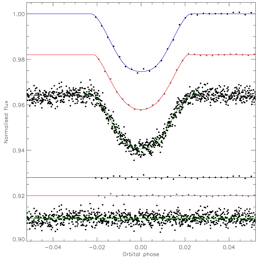
TrES-3 was discovered by O’Donovan et al. (2007) and previously studied in Paper III. Since then interleaved light curves of one transit have been published in two narrow passbands, with central wavelengths 790.2 nm and 794.4 nm, by Colón et al. (2010), photometry of four transits has been presented by Lee et al. (2011), and a light curve from the Deep Impact mission has been obtained in the course of the EPOCH project (Christiansen et al., 2011). In the current work I improve upon the results from Paper III (see fig. 12 in that work) by studying the data from Colón et al. (2010) and Christiansen et al. (2011).

The 790.2 nm and 794.4 nm light curves cover the same transit by alternating between the two passbands using a tunable filter. In both cases (Tables A113 and A114) correlated noise is unimportant and LD-fit/fix provides the best solution.

The EPOCH data cover six transits, of which one has only partial coverage and one has problems with systematic noise. The 1171 datapoints in the region of the remaining four transits were selected and four were rejected by a 3.5$\sigma$ clip. Table A115 shows that the LD-fit/fix solutions return questionable results, so the LD-fixed solutions had to be adopted. Unusually for the EPOCH data, the residual-permutation errorbars were not larger than the Monte-Carlo ones.

The final results for each light curve are given in Table A116, alongside the results for the seven light curves investigated in Paper III. Fig. 35 shows the best fits. The final photometric parameters were obtained by multiplying the probability density functions for the ten light curves from Paper III and the current work. The agreement between light curves and with literature values is excellent. The physical properties of TrES-3 can be found in Table A117 and again show good correspondance with published numbers. TrES-3 is well-characterised, but would benefit from a few more RV measurements.

6.30 WASP-3

Figure 36: Phased light curves of WASP-3 compared to the best fits found using jktebop and the quadratic LD law. From top to bottom the datasets are $g$ then $i$ then $z$ from Tripathi et al. (2010), and the EPOCH data from Christiansen et al. (2011). See Fig. 26 for further details. See Paper III (fig. 14 and sect. 4.10) for previous results.

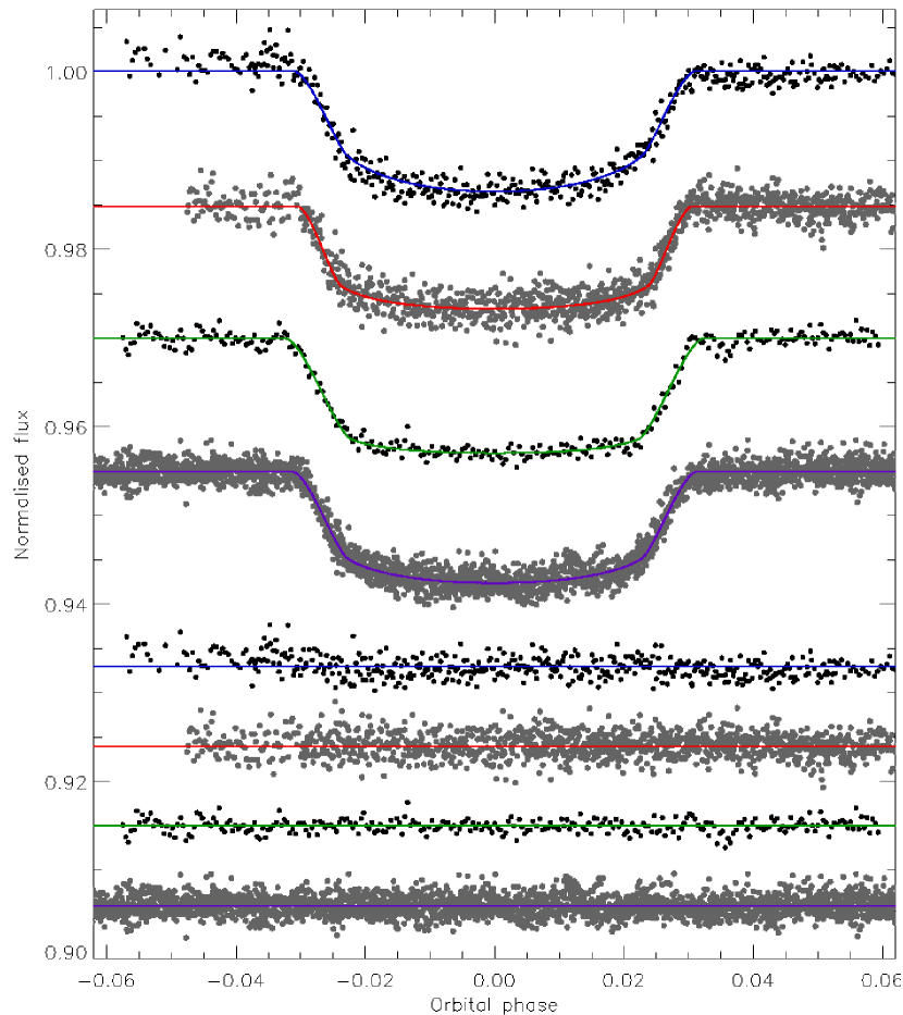
WASP-3 was treated in Paper III but is revisited here, as it has since been observed from the ground by Tripathi et al. (2010) and from space by Christiansen et al. (2011). Six nice transit light curves were obtained by Tripathi et al. (2010), comprising three in $i$ and two in $g$ from the FLWO 1.2 m and one in $z$ from the University of Hawaii 2.2 m. The Christiansen et al. (2011) data come from EPOCH and cover eight transits with good precision but some systematics due to pointing wander and imperfect flat-fielding. Maciejewski et al. (2010) has detected possible TTVs in the WASP-3 system, which are yet to be independently confirmed.

I adopt the same $T_{\rm eff}$ and $\left[\frac{\rm Fe}{\rm H}\right]$ as in Paper I (Pollacco et al., 2008). Two RV studies exist for WASP-3, yielding velocity amplitudes of $290.5\pm 9.5$ m s^-1 (Tripathi et al., 2010) and $278.2\pm 13.6$ m s^-1 (Miller et al., 2010). In Paper III I took the former of these two values, but in the current work I adopted instead the weighted mean: $K_{\rm A}=286.5\pm 7.8$ m s^-1.

The $g$-band data contain two transits so the $P_{\rm orb}$ was included in the fit to insure against possible bias from TTV effects. The LD-fit/fix solutions are best and the residual-permutation errorbars are about 30% larger than the Monte-Carlo ones (Table A118). The $i$-band data cover three transits so $P_{\rm orb}$ was again fitted for. The LD-fit/fix solutions are good and correlated noise is not important (Table A119). The $z$-band data encompass one transit; LD-fit/fix values were adopted and the residual-permutation errorbars are 25% larger than Monte-Carlo (Table A120. The EPOCH data cover eight transits, of which one was rejected due to poor observational coverage, with 18 622 datapoints. 3397 are near transit, of which 34 fell foul of a 3.5$\sigma$ clip. The LD-fit/fix results were retained and the residual-permutation errorbars are 40% larger than the Monte Carlo ones (Table A121).

Fig. 36 shows best fits of the four light curves. Table A122 summarises the photometric results from the current work and from Paper III. All seven light curves are used to calculate the final photometric parameters, which are mostly in good agreement. The $k$ values are more scattered than they should be ($\chi_{\nu}^{\,2}=5.4$) and this has a knock-on effect on $r_{\rm b}$ which has been accounted for in the errorbars. Other works are in good agreement with my results, albeit with unreasonably small errorbars in some cases. An exception is Miller et al. (2010) who find a discrepant solution with high inclination and thus lower $r_{\rm A}$. This situation propagates into the physical properties (Table A123), which are now substantially improved over those in Paper III. Further spectroscopic observations, both for RV and atmospheric parameter measurements, are warranted.

6.31 Other TEPs

I have returned to the XO-4 system, which has received a new and substantially improved $K_{\rm A}$ measurement from Narita et al. (2010) since Paper III. Table A124 shows the revision in the system parameters this brings.

Finally, I have checked that the modifications to the jktabsdim code outlined in Sect. 3.1 (primarily the much better sampling in age) by rerunning solutions for the WASP-7 system (Southworth et al., 2011). The new results are almost identical to the old ones (Table A125), except for the correction to $\rho_{\rm b}$ discussed in Sect. 3.3. The full set of homogeneous properties for transiting extrasolar planetary systems can now be accessed by considering only the current work and Paper III.

7 Performance of the dEB relation versus constraints from theoretical models

Figure 37: Comparisons between the $K_{\rm b}$ values obtained using individual sets of stellar evolutionary models and the unweighted mean value, $\langle$$K_{\rm b}$$\rangle$, for each TEP. From left to right the panels show results for the dEB constraint and then the five stellar model sets. The top panels compare $K_{\rm b}$ to $\langle$$K_{\rm b}$$\rangle$ for each model set, with parity indicated by a dotted line. Lower panels show the difference ($K_{\rm b}-\langle$$K_{\rm b}$$\rangle$) as a function of $T_{\rm eff}$, $\left[\frac{\rm Fe}{\rm H}\right]$ and $M_{\rm A}$.

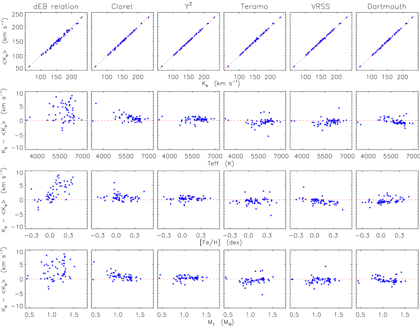
One of the new procedures introduced in the current work is an optional constraint using a $R_{\rm A}=f(M_{\rm A},T_{\rm eff},\left[\frac{\rm Fe}{\rm H}\right])$ relation obtained from well-studied dEBs and following the method of Enoch et al. (2010). This replaces the approach used in Papers II and III, which utilised a mass–radius relation from dEBs, which was simpler but did not work very well. The cost is a reliance on $T_{\rm eff}$ and $\left[\frac{\rm Fe}{\rm H}\right]$ measurements, which incurs a dependence on theoretical model atmospheres. The new approach gives results in much better agreement with those found via theoretical models.

The dEB constraint has been used to calculate physical properties for the 30 TEPs studied in Paper III, giving a sample of 58 TEPs with physical properties calculated in several ways: using the dEB constraint, using each of five different theoretical model tabulations, and the nominal results which are an unweighted mean of the ones from the five model sets. The parameter $K_{\rm b}$ is well-suited for comparing the different options, as it is the solution control parameter in jktabsdim and wholly encompasses the outside constraints used in calculating the physical properties. A larger $K_{\rm b}$ results in larger numbers for all of the physical properties (see eqs. 4 to 12 in Paper II) with the exceptions of $\Theta$ (which gets smaller) and the three quantities which have no model dependence ($g_{\rm b}$, $\rho_{\rm A}$ and $T_{\rm eq}^{\,\prime}$).

Fig. 37 presents a detailed visualisation of the $K_{\rm b}$ values obtained from the various solutions for each TEP system. This Figure is a modified version of fig. 20 in Paper III with double the number of systems and with the dEB constraint instead of the mass–radius constraint. Previous assertions can be confirmed: the Claret models yield a larger $K_{\rm b}$ on average, the VRSS models give a lower $K_{\rm b}$ on average, and the Y² models show no trends with $T_{\rm eff}$, $\left[\frac{\rm Fe}{\rm H}\right]$ and $M_{\rm A}$ compared to the mean model solution. The dEB constraint is clearly hugely more successful than the mass–radius relation in reproducing the theoretical model results, but tends to return a larger $K_{\rm b}$ particularly at high metallicity. This confirms that it is a useful tool in quick calculation of the properties of transiting planets.

8 Physical properties of the transiting extrasolar planetary systems

Figure 38: Plot of the masses versus the radii of the stars in the 58 TEPs with homogeneous properties. The statistical uncertainties are shown by black open diamonds and the systematic uncertainties by red filled diamonds. The empirical mass–radius relation from Paper II is shown with a blue line.

Figure 39: Plot of the masses versus the radii of the planets in the 58 TEPs with homogeneous properties. The statistical uncertainties are shown by black open diamonds and the systematic uncertainties by red filled diamonds. Blue dotted lines show where density is 1.0, 0.5 and 0.25 $\,\rho_{\rm Jup}$.

Figure 40: Plot of the masses versus the radii of all published TEPs and their host stars. Blue crosses show the objects studied in the current series of papers and red crosses show results taken from the literature. The Solar system bodies are shown by green filled circles. The grey dotted lines show the loci where density is equal to $\,\rho_{\rm Jup}$ (upper line) and $\,\rho_{\odot}$ (lower line).

Table 6: Physical properties of the stellar components of the TEPs studied in this work. For each quantity the first uncertainty is derived from a propagation of all observational errors and the second uncertainty is an estimate of the systematic errors arising from the dependence on stellar theory.

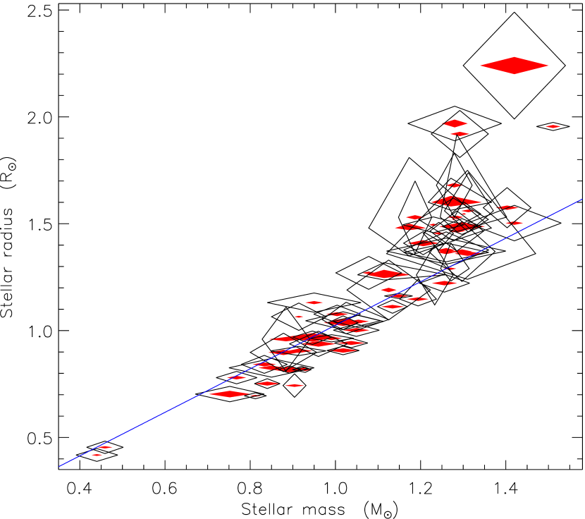
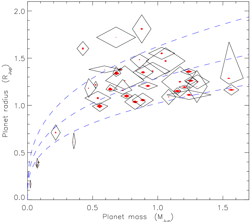
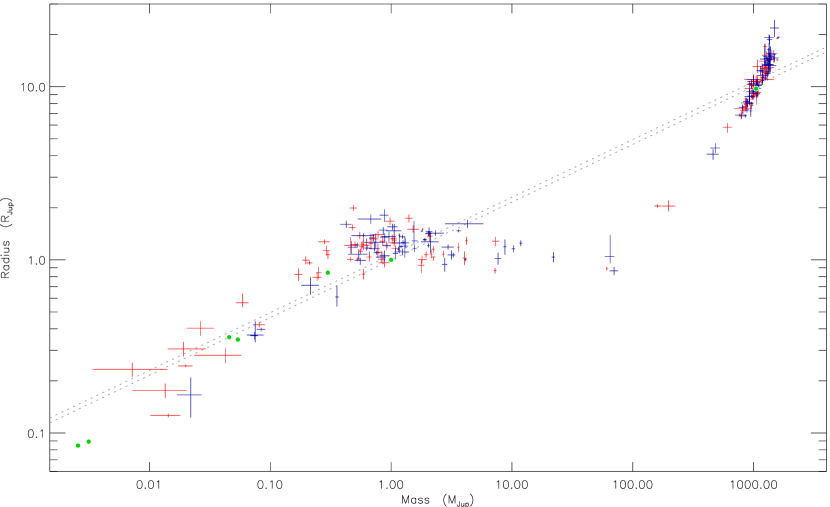
System

Semimajor axis (AU)

Mass ($\,{\rm M}_{\odot}$)

Radius ($\,{\rm R}_{\odot}$)

$\log g_{\rm A}$ [cm/s]

Density ($\,\rho_{\odot}$)

Age (Gyr)

CoRoT-1

0.02536 $\pm$

0.00098 $\pm$

0.00016

0.95 $\pm$

0.11 $\pm$

0.02

1.131 $\pm$

0.045 $\pm$

0.007

4.311 $\pm$

0.019 $\pm$

0.003

$0.660\pm 0.019$

${7.8\,^{+4.0}_{-3.8}}\,^{+0.7}_{-0.7}$

CoRoT-2

0.02854 $\pm$

0.00036 $\pm$

0.00032

1.018 $\pm$

0.038 $\pm$

0.034

0.907 $\pm$

0.020 $\pm$

0.010

4.530 $\pm$

0.015 $\pm$

0.005

$1.362\pm 0.064$

${0.6\,^{+1.9}_{-2.1}}\,^{+1.5}_{-0.6}$

CoRoT-3

0.05783 $\pm$

0.00078 $\pm$

0.00035

1.403 $\pm$

0.056 $\pm$

0.026

1.575 $\pm$

0.094 $\pm$

0.010

4.191 $\pm$

0.046 $\pm$

0.003

$0.359\pm 0.058$

${1.5\,^{+0.5}_{-0.5}}\,^{+0.3}_{-0.2}$

CoRoT-4

${0.09120\,^{+0.00110}_{-0.00112}}\,^{+0.00061}_{-0.00067}$

${1.194\,^{+0.043}_{-0.043}}\,^{+0.024}_{-0.026}$

${1.1475\,^{+0.0923}_{-0.0322}}\,^{+0.0077}_{-0.0084}$

${4.3959\,^{+0.0237}_{-0.0678}}\,^{+0.0029}_{-0.0032}$

$0.790^{+0.064}_{-0.161}$

${0.8\,^{+2.6}_{-1.0}}\,^{+0.6}_{-0.3}$

CoRoT-5

${0.05004\,^{+0.00161}_{-0.00092}}\,^{+0.00022}_{-0.00033}$

${1.025\,^{+0.100}_{-0.056}}\,^{+0.013}_{-0.020}$

${1.0516\,^{+0.0810}_{-0.0666}}\,^{+0.0045}_{-0.0069}$

${4.4053\,^{+0.0683}_{-0.0594}}\,^{+0.0019}_{-0.0028}$

$0.88^{+0.21}_{-0.16}$

${3.9\,^{+2.6}_{-5.3}}\,^{+0.6}_{-1.0}$

CoRoT-6

0.0855 $\pm$

0.0016 $\pm$

0.0007

1.054 $\pm$

0.059 $\pm$

0.024

1.043 $\pm$

0.029 $\pm$

0.008

4.425 $\pm$

0.022 $\pm$

0.003

$0.929\pm 0.064$

${2.5\,^{+2.1}_{-1.7}}\,^{+0.6}_{-0.7}$

CoRoT-7

0.01690 $\pm$

0.00036 $\pm$

0.00025

0.884 $\pm$

0.056 $\pm$

0.039

0.96 $\pm$

0.15 $\pm$

0.01

4.42 $\pm$

0.14 $\pm$

0.01

$1.00\pm 0.48$

unconstrained

CoRoT-8

0.0633 $\pm$

0.0019 $\pm$

0.0008

0.878 $\pm$

0.078 $\pm$

0.035

0.898 $\pm$

0.090 $\pm$

0.012

4.475 $\pm$

0.077 $\pm$

0.006

$1.21\pm 0.32$

unconstrained

CoRoT-9

0.4027 $\pm$

0.0095 $\pm$

0.0056

0.960 $\pm$

0.068 $\pm$

0.040

0.938 $\pm$

0.059 $\pm$

0.013

4.476 $\pm$

0.063 $\pm$

0.006

$1.16\pm 0.24$

unconstrained

CoRoT-10

0.1060 $\pm$

0.0011 $\pm$

0.0009

0.904 $\pm$

0.027 $\pm$

0.022

0.743 $\pm$

0.055 $\pm$

0.006

4.652 $\pm$

0.062 $\pm$

0.004

$2.20\pm 0.47$

${0.1\,^{+2.0}_{-0.2}}\,^{+0.3}_{-0.1}$

CoRoT-11

0.0440 $\pm$

0.0016 $\pm$

0.0003

1.26 $\pm$

0.14 $\pm$

0.02

1.374 $\pm$

0.061 $\pm$

0.009

4.264 $\pm$

0.019 $\pm$

0.003

$0.488\pm 0.022$

${2.0\,^{+0.8}_{-2.1}}\,^{+0.4}_{-0.4}$

CoRoT-12

0.0394 $\pm$

0.0011 $\pm$

0.0004

1.018 $\pm$

0.088 $\pm$

0.029

1.046 $\pm$

0.042 $\pm$

0.010

4.407 $\pm$

0.029 $\pm$

0.004

$0.889\pm 0.076$

${5.8\,^{+3.3}_{-6.7}}\,^{+1.8}_{-1.5}$

CoRoT-13

0.0510 $\pm$

0.0012 $\pm$

0.0005

1.086 $\pm$

0.077 $\pm$

0.035

1.274 $\pm$

0.077 $\pm$

0.014

4.264 $\pm$

0.040 $\pm$

0.005

$0.526\pm 0.072$

${5.8\,^{+1.4}_{-6.2}}\,^{+0.5}_{-1.0}$

CoRoT-14

0.02687 $\pm$

0.00077 $\pm$

0.00015

1.125 $\pm$

0.098 $\pm$

0.018

1.19 $\pm$

0.14 $\pm$

0.01

4.338 $\pm$

0.082 $\pm$

0.002

$0.67\pm 0.19$

${3.7\,^{+2.5}_{-5.0}}\,^{+0.7}_{-0.6}$

CoRoT-15

${0.0458\,^{+0.0018}_{-0.0022}}\,^{+0.0005}_{-0.0003}$

${1.31\,^{+0.16}_{-0.19}}\,^{+0.04}_{-0.03}$

${1.36\,^{+0.39}_{-0.12}}\,^{+0.01}_{-0.01}$

${4.288\,^{+0.059}_{-0.191}}\,^{+0.005}_{-0.003}$

$0.52^{+0.12}_{-0.25}$

${1.6\,^{+4.5}_{-5.9}}\,^{+0.9}_{-1.6}$

HAT-P-4

${0.04465\,^{+0.00113}_{-0.00062}}\,^{+0.00084}_{-0.00054}$

${1.271\,^{+0.096}_{-0.053}}\,^{+0.072}_{-0.046}$

${1.600\,^{+0.113}_{-0.037}}\,^{+0.030}_{-0.019}$

${4.134\,^{+0.015}_{-0.038}}\,^{+0.008}_{-0.005}$

$0.310^{+0.016}_{-0.041}$

${3.9\,^{+0.6}_{-0.9}}\,^{+0.6}_{-1.1}$

HAT-P-7

0.03805 $\pm$

0.00033 $\pm$

0.00015

1.511 $\pm$

0.039 $\pm$

0.017

1.955 $\pm$

0.019 $\pm$

0.007

4.0354 $\pm$

0.0049 $\pm$

0.0017

$0.2023\pm 0.0024$

${2.0\,^{+0.4}_{-0.3}}\,^{+0.3}_{-0.2}$

HAT-P-11

0.05259 $\pm$

0.00056 $\pm$

0.00027

0.812 $\pm$

0.026 $\pm$

0.012

0.695 $\pm$

0.014 $\pm$

0.004

4.663 $\pm$

0.012 $\pm$

0.002

$2.415\pm 0.097$

unconstrained

HD 17156

0.1637 $\pm$

0.0019 $\pm$

0.0022

1.297 $\pm$

0.046 $\pm$

0.053

1.487 $\pm$

0.037 $\pm$

0.020

4.207 $\pm$

0.018 $\pm$

0.006

$0.395\pm 0.022$

${2.8\,^{+1.1}_{-0.6}}\,^{+0.4}_{-0.4}$

HD 80606

0.4564 $\pm$

0.0054 $\pm$

0.0068

1.018 $\pm$

0.035 $\pm$

0.045

1.037 $\pm$

0.032 $\pm$

0.015

4.415 $\pm$

0.021 $\pm$

0.007

$0.913\pm 0.062$

${5.9\,^{+1.6}_{-2.2}}\,^{+4.1}_{-2.1}$

Kepler-4

${0.0449\,^{+0.0024}_{-0.0012}}\,^{+0.0005}_{-0.0004}$

${1.173\,^{+0.193}_{-0.095}}\,^{+0.039}_{-0.033}$

${1.48\,^{+0.33}_{-0.13}}\,^{+0.02}_{-0.01}$

${4.168\,^{+0.063}_{-0.133}}\,^{+0.005}_{-0.004}$

$0.362^{+0.081}_{-0.136}$

${5.3\,^{+1.5}_{-2.5}}\,^{+0.4}_{-0.4}$

Kepler-5

${0.04967\,^{+0.00051}_{-0.00038}}\,^{+0.00014}_{-0.00028}$

${1.296\,^{+0.040}_{-0.030}}\,^{+0.011}_{-0.022}$

${1.544\,^{+0.055}_{-0.042}}\,^{+0.004}_{-0.009}$

${4.174\,^{+0.023}_{-0.024}}\,^{+0.001}_{-0.002}$

$0.352^{+0.025}_{-0.029}$

${2.8\,^{+0.3}_{-0.5}}\,^{+0.3}_{-0.3}$

Kepler-6

${0.04438\,^{+0.00181}_{-0.00081}}\,^{+0.00080}_{-0.00053}$

${1.114\,^{+0.146}_{-0.062}}\,^{+0.061}_{-0.040}$

${1.261\,^{+0.057}_{-0.024}}\,^{+0.023}_{-0.015}$

${4.284\,^{+0.017}_{-0.011}}\,^{+0.008}_{-0.005}$

$0.5555^{+0.0076}_{-0.0209}$

${5.7\,^{+0.8}_{-2.3}}\,^{+0.3}_{-0.5}$

Kepler-7

0.0613 $\pm$

0.0017 $\pm$

0.0006

1.28 $\pm$

0.11 $\pm$

0.03

1.969 $\pm$

0.081 $\pm$

0.018

3.959 $\pm$

0.024 $\pm$

0.004

$0.168\pm 0.012$

${4.4\,^{+0.4}_{-1.6}}\,^{+0.7}_{-0.4}$

Kepler-8

0.0485 $\pm$

0.0012 $\pm$

0.0002

1.230 $\pm$

0.072 $\pm$

0.01

1.495 $\pm$

0.037 $\pm$

0.005

4.178 $\pm$

0.022 $\pm$

0.002

$0.368\pm 0.014$

${3.2\,^{+1.8}_{-3.1}}\,^{+0.6}_{-1.1}$

KOI-428

0.0795 $\pm$

0.0022 $\pm$

0.0015

1.42 $\pm$

0.12 $\pm$

0.08

2.24 $\pm$

0.25 $\pm$

0.04

3.889 $\pm$

0.099 $\pm$

0.008

$0.126\pm 0.042$

${2.1\,^{+0.6}_{-0.6}}\,^{+0.1}_{-0.3}$

LHS 6343

0.0850 $\pm$

0.0031 $\pm$

0.0007

0.440 $\pm$

0.049 $\pm$

0.012

0.418 $\pm$

0.030 $\pm$

0.004

4.839 $\pm$

0.035 $\pm$

0.004

$6.01\pm 0.76$

${4.0\,^{+0.7}_{-0.0}}\,^{+2.0}_{-3.0}$

TrES-2

0.03567 $\pm$

0.00061 $\pm$

0.00029

0.991 $\pm$

0.052 $\pm$

0.024

0.964 $\pm$

0.017 $\pm$

0.008

4.4660 $\pm$

0.0081 $\pm$

0.0035

$1.105\pm 0.011$

${3.4\,^{+2.0}_{-2.2}}\,^{+0.5}_{-0.5}$

TrES-3

0.02276 $\pm$

0.00012 $\pm$

0.00011

0.921 $\pm$

0.014 $\pm$

0.014

0.8235 $\pm$

0.0098 $\pm$

0.0040

4.5710 $\pm$

0.0064 $\pm$

0.0021

$1.648\pm 0.041$

${1.0\,^{+0.5}_{-0.0}}\,^{+0.0}_{-0.0}$

WASP-3

0.03185 $\pm$

0.00086 $\pm$

0.00020

1.26 $\pm$

0.10 $\pm$

0.02

1.366 $\pm$

0.044 $\pm$

0.008

4.268 $\pm$

0.018 $\pm$

0.003

$0.495\pm 0.024$

${2.1\,^{+1.2}_{-1.2}}\,^{+0.4}_{-0.4}$

WASP-7

0.0619 $\pm$

0.0010 $\pm$

0.0003

1.285 $\pm$

0.063 $\pm$

0.019

1.466 $\pm$

0.094 $\pm$

0.007

4.215 $\pm$

0.046 $\pm$

0.002

$0.408\pm 0.068$

${2.5\,^{+0.8}_{-0.9}}\,^{+0.2}_{-0.4}$

XO-4

${0.05474\,^{+0.00162}_{-0.00056}}\,^{+0.00020}_{-0.00031}$

${1.285\,^{+0.117}_{-0.039}}\,^{+0.014}_{-0.022}$

${1.531\,^{+0.386}_{-0.068}}\,^{+0.006}_{-0.009}$

${4.177\,^{+0.034}_{-0.172}}\,^{+0.002}_{-0.002}$

$0.358^{+0.046}_{-0.160}$

${2.7\,^{+1.1}_{-0.5}}\,^{+0.2}_{-0.3}$

Table 7: Physical properties of the planetary components of the TEPs studied in this work. For each quantity the first uncertainty is derived from a propagation of all observational errors and the second uncertainty is an estimate of the systematic errors arising from the dependence on stellar theory.

System

Mass ($\,{\rm M}_{\rm Jup}$)

Radius ($\,{\rm R}_{\rm Jup}$)

$g_{\rm b}$ ( m s-2)

Density ($\,\rho_{\rm Jup}$)

$T_{\rm eq}^{\,\prime}$ (K)

$\Theta$

CoRoT-1

1.03  $\pm$

0.10  $\pm$

0.01

1.551  $\pm$

0.064  $\pm$

0.010

$10.65\pm 0.69$

0.259  $\pm$

0.021  $\pm$

0.002

$1915\pm 49$

0.0354  $\pm$

0.0025  $\pm$

0.0002

CoRoT-2

3.62  $\pm$

0.14  $\pm$

0.08

1.470  $\pm$

0.028  $\pm$

0.016

$41.5\pm 1.7$

1.066  $\pm$

0.057  $\pm$

0.012

$1548\pm 22$

0.1381  $\pm$

0.0049  $\pm$

0.0016

CoRoT-3

21.96  $\pm$

0.65  $\pm$

0.27

1.037  $\pm$

0.069  $\pm$

0.006

$506\pm 67$

18.4  $\pm$

3.7  $\pm$

0.1

$1695\pm 57$

1.74  $\pm$

0.12  $\pm$

0.01

CoRoT-4

${0.731\,^{+0.072}_{-0.073}}\,^{+0.0010}_{-0.011}$

${1.160\,^{+0.116}_{-0.041}}\,^{+0.008}_{-0.009}$

$13.5^{+1.6}_{-2.6}$

${0.438\,^{+0.063}_{-0.117}}\,^{+0.003}_{-0.003}$

$1058^{+42}_{-17}$

${0.0962\,^{+0.0099}_{-0.0127}}\,^{+0.0007}_{-0.0006}$

CoRoT-5

${0.470\,^{+0.058}_{-0.031}}\,^{+0.004}_{-0.006}$

${1.182\,^{+0.102}_{-0.098}}\,^{+0.005}_{-0.008}$

$8.3^{+1.8}_{-1.3}$

${0.266\,^{+0.082}_{-0.058}}\,^{+0.002}_{-0.001}$

$1348^{+50}_{-51}$

${0.0388\,^{+0.0054}_{-0.0038}}\,^{+0.0003}_{-0.0002}$

CoRoT-6

2.96  $\pm$

0.34  $\pm$

0.05

1.185  $\pm$

0.041  $\pm$

0.009

$52.3\pm 6.4$

1.66  $\pm$

0.23  $\pm$

0.01

$1025\pm 16$

0.405  $\pm$

0.046  $\pm$

0.003

CoRoT-7

0.0220  $\pm$

0.0050  $\pm$

0.0007

0.166  $\pm$

0.043  $\pm$

0.002

$19\pm 12$

4.5  $\pm$

4.5  $\pm$

0.1

$1910\pm 140$

0.0051  $\pm$

0.0018  $\pm$

0.0001

CoRoT-8

0.216  $\pm$

0.036  $\pm$

0.006

0.712  $\pm$

0.083  $\pm$

0.010

$10.6\pm 2.9$

0.56  $\pm$

0.21  $\pm$

0.01

$922\pm 41$

0.0437  $\pm$

0.0084  $\pm$

0.0006

CoRoT-9

0.826  $\pm$

0.080  $\pm$

0.023

1.037  $\pm$

0.081  $\pm$

0.014

$19.1\pm 3.2$

0.69  $\pm$

0.17  $\pm$

0.01

$413\pm 14$

0.668  $\pm$

0.076  $\pm$

0.009

CoRoT-10

2.78  $\pm$

0.14  $\pm$

0.05

0.941  $\pm$

0.085  $\pm$

0.008

$78\pm 14$

3.13  $\pm$

0.88  $\pm$

0.03

$647\pm 24$

0.693  $\pm$

0.070  $\pm$

0.006

CoRoT-11

2.34  $\pm$

0.39  $\pm$

0.03

1.426  $\pm$

0.057  $\pm$

0.009

$28.5\pm 4.2$

0.76  $\pm$

0.12  $\pm$

0.00

$1735\pm 34$

0.114  $\pm$

0.017  $\pm$

0.001

CoRoT-12

0.887  $\pm$

0.077  $\pm$

0.017

1.350  $\pm$

0.074  $\pm$

0.013

$12.1\pm 1.3$

0.337  $\pm$

0.052  $\pm$

0.003

$1410\pm 28$

0.0508  $\pm$

0.0042  $\pm$

0.0005

CoRoT-13

1.312  $\pm$

0.092  $\pm$

0.028

1.252  $\pm$

0.075  $\pm$

0.013

$20.7\pm 2.5$

0.62  $\pm$

0.11  $\pm$

0.01

$1432\pm 39$

0.0983  $\pm$

0.0080  $\pm$

0.0010

CoRoT-14

7.67  $\pm$

0.49  $\pm$

0.08

1.018  $\pm$

0.079  $\pm$

0.005

$183\pm 27$

6.8  $\pm$

1.5  $\pm$

0.0

$1936\pm 95$

0.360  $\pm$

0.030  $\pm$

0.002

CoRoT-15

${64.9\,^{+5.3}_{-6.2}}\,^{+1.3}_{-1.0}$

${1.045\,^{+0.347}_{-0.091}}\,^{+0.011}_{-0.008}$

$1470^{+240}_{-620}$

${53\,^{+13}_{-29}}\,^{+0}_{-0}$

$1670^{+200}_{-80}$

${4.34\,^{+0.41}_{-1.07}}\,^{+0.03}_{-0.05}$

HAT-P-4

${0.680\,^{+0.038}_{-0.025}}\,^{+0.026}_{-0.016}$

${1.337\,^{+0.075}_{-0.032}}\,^{+0.025}_{-0.016}$

$9.42^{+0.44}_{-0.91}$

${0.266\,^{+0.018}_{-0.038}}\,^{+0.003}_{-0.005}$

$1691^{+46}_{-26}$

${0.0357\,^{+0.0012}_{-0.0021}}\,^{+0.0004}_{-0.0007}$

HAT-P-7

1.799  $\pm$

0.038  $\pm$

0.014

1.465  $\pm$

0.015  $\pm$

0.006

$20.77\pm 0.33$

0.535  $\pm$

0.011  $\pm$

0.002

$2194\pm 27$

0.0618  $\pm$

0.0010  $\pm$

0.0002

HAT-P-11

0.084  $\pm$

0.007  $\pm$

0.001

0.397  $\pm$

0.009  $\pm$

0.002

$13.2\pm 1.1$

1.26  $\pm$

0.12  $\pm$

0.01

$838\pm 10$

0.0274  $\pm$

0.0022  $\pm$

0.0001

HD 17156

3.262  $\pm$

0.072  $\pm$

0.088

1.065  $\pm$

0.033  $\pm$

0.014

$71.2\pm 3.7$

2.52  $\pm$

0.20  $\pm$

0.03

$883\pm 11$

0.772  $\pm$

0.026  $\pm$

0.010

HD 80606

4.114  $\pm$

0.096  $\pm$

0.122

1.003  $\pm$

0.023  $\pm$

0.015

$101.4\pm 3.9$

3.82  $\pm$

0.23  $\pm$

0.06

$405.0\pm 7.0$

3.677  $\pm$

0.093  $\pm$

0.055

Kepler-4

${0.075\,^{+0.013}_{-0.011}}\,^{+0.002}_{-0.001}$

${0.368\,^{+0.074}_{-0.034}}\,^{+0.004}_{-0.003}$

$13.8^{+3.3}_{-4.5}$

${1.41\,^{+0.48}_{-0.62}}\,^{+0.01}_{-0.02}$

$1620^{+140}_{-60}$

${0.0156\,^{+0.0025}_{-0.0034}}\,^{+0.0001}_{-0.0002}$

Kepler-5

${2.040\,^{+0.048}_{-0.040}}\,^{+0.006}_{-0.007}$

${1.210\,^{+0.035}_{-0.030}}\,^{+0.002}_{-0.002}$

$34.5^{+1.7}_{-1.9}$

${1.076\,^{+0.080}_{-0.086}}\,^{+0.002}_{-0.001}$

$1692^{+29}_{-25}$

${0.1286\,^{+0.0036}_{-0.0040}}\,^{+0.0002}_{-0.0002}$

Kepler-6

${0.633\,^{+0.057}_{-0.031}}\,^{+0.023}_{-0.015}$

${1.169\,^{+0.052}_{-0.022}}\,^{+0.021}_{-0.014}$

$11.48^{+0.39}_{-0.54}$

${0.370\,^{+0.015}_{-0.026}}\,^{+0.004}_{-0.007}$

$1451^{+15}_{-13}$

${0.0431\,^{+0.0016}_{-0.0022}}\,^{+0.0005}_{-0.0008}$

Kepler-7

0.425  $\pm$

0.046  $\pm$

0.008

1.602  $\pm$

0.075  $\pm$

0.014

$4.10\pm 0.43$

0.097  $\pm$

0.013  $\pm$

0.001

$1621\pm 23$

0.0253  $\pm$

0.0024  $\pm$

0.0002

Kepler-8

0.59  $\pm$

0.12  $\pm$

0.00

1.381  $\pm$

0.037  $\pm$

0.005

$7.7\pm 1.4$

0.210  $\pm$

0.040  $\pm$

0.001

$1662\pm 41$

0.0337  $\pm$

0.0063  $\pm$

0.0001

KOI-428

2.12  $\pm$

0.35  $\pm$

0.08

1.27  $\pm$

0.17  $\pm$

0.02

$32\pm 10$

0.98  $\pm$

0.44  $\pm$

0.02

$1666\pm 92$

0.188  $\pm$

0.038  $\pm$

0.003

LHS 6343

69.9  $\pm$

5.6  $\pm$

1.2

0.864  $\pm$

0.048  $\pm$

0.007

$2320\pm 210$

101  $\pm$

13  $\pm$

0

$352\pm 22$

31.2  $\pm$

2.2  $\pm$

0.3

TrES-2

1.206  $\pm$

0.045  $\pm$

0.020

1.193  $\pm$

0.021  $\pm$

0.010

$21.02\pm 0.31$

0.665  $\pm$

0.015  $\pm$

0.005

$1466\pm 12$

0.0727  $\pm$

0.0017  $\pm$

0.0006

TrES-3

1.899  $\pm$

0.060  $\pm$

0.019

1.310  $\pm$

0.019  $\pm$

0.006

$27.4\pm 1.1$

0.790  $\pm$

0.040  $\pm$

0.004

$1638\pm 22$

0.0716  $\pm$

0.0024  $\pm$

0.0004

WASP-3

2.03  $\pm$

0.12  $\pm$

0.03

1.416  $\pm$

0.047  $\pm$

0.009

$25.1\pm 1.2$

0.669  $\pm$

0.047  $\pm$

0.004

$2020\pm 35$

0.0724  $\pm$

0.0031  $\pm$

0.0004

WASP-7

0.96  $\pm$

0.13  $\pm$

0.01

1.363  $\pm$

0.093  $\pm$

0.007

$12.9\pm 2.4$

0.356  $\pm$

0.087  $\pm$

0.002

$1502\pm 47$

0.068  $\pm$

0.010  $\pm$

0.000

XO-4

${1.547\,^{+0.110}_{-0.066}}\,^{+0.011}_{-0.017}$

${1.287\,^{+0.385}_{-0.063}}\,^{+0.005}_{-0.007}$

$23.1^{+2.5}_{-9.4}$

${0.68\,^{+0.11}_{-0.37}}\,^{+0.00}_{-0.00}$

$1630^{+170}_{-40}$

${0.1023\,^{+0.0065}_{-0.0240}}\,^{+0.0006}_{-0.0004}$

The major results of this work are the physical properties of 32 transiting extrasolar planetary systems obtained using homogeneous methods and by combining all available photometric data (Table 4) with measured spectroscopic parameters of the host stars (Table 5). The stellar properties are given in Table 6 and the planetary ones in Table 7. These quantities supplement (and in few cases supersede) the properties for 30 objects found in Paper III, giving a total sample of 58 systems. The homogeneous nature of these results means they are well suited for comparing different TEPs, for planning follow-up observations, and for performing detailed statistical studies.

Figs. 38 and 39 show the masses and radii of the stars and planets with their random (black open diamonds) and systematic (red filled diamonds) errorbars. It is clear that the property of these four which is most affected by systematic error is $M_{\rm A}$, whereas the masses and radii of the planets are not strongly affected by this model dependence, as previously found in Paper III.

Fig. 40 shows the masses and radii of the TEPs and their host stars on the same plot. The plot includes all 118 TEP systems known as of 2011/04/19 and includes the 58 systems studied in this series of papers plus results taken from the literature for the other 60 systems. The Sun, Jupiter, Saturn, Uranus, Neptune, Earth and Venus are also plotted for context, as are lines denoting the points where density is equal to $\,\rho_{\rm Jup}$ and $\,\rho_{\odot}$. Fig. 40 clearly highlights the wide range of parameter space covered by these systems, as well as the fact that the properties of the planets are much more scattered than those of the parent stars.

9 Follow-up observations

Table 8: Summary of which types of additional observations would be useful for the thirty TEPs studied in this work. $\star$ denotes where additional data would be useful, and $\star\star$ indicates where it would be useful but difficult to either obtain or interpret.

System	Photometric	Radial	Spectral
	observations	velocities	synthesis
CoRoT-1		$\star$	$\star$
CoRoT-2		$\star$	$\star$
CoRoT-3	$\star\star$		$\star$
CoRoT-4	$\star\star$	$\star$
CoRoT-5		$\star$	$\star$
CoRoT-6		$\star$	$\star$
CoRoT-7	$\star\star$	$\star\star$
CoRoT-8	$\star$	$\star\star$
CoRoT-9
CoRoT-10	$\star\star$
CoRoT-11		$\star\star$	$\star$
CoRoT-12	$\star\star$		$\star$
CoRoT-13		$\star$
CoRoT-14	$\star\star$		$\star\star$
CoRoT-15		$\star\star$	$\star\star$
HAT-P-4	$\star$
HAT-P-7
HAT-P-11
HD 17156
HD 80606
Kepler-4	$\star$	$\star$	$\star$
Kepler-5
Kepler-6		$\star$
Kepler-7	$\star$
Kepler-8		$\star$	$\star$
KOI-428	$\star$	$\star$	$\star$
LHS 6343	$\star$	$\star$	$\star$
TrES-2			$\star$
TrES-3	$\star$
WASP-3		$\star$	$\star$
WASP-7	$\star$	$\star$	$\star$
XO-4	$\star$

Most of the TEPs in the current work would benefit from further observations of some sort. In many cases the dominant uncertainty stems from the quality of the light curve. This remains true for many of the CoRoT systems, despite their space-based light curves. It must be remembered that CoRoT has only a 27 cm diameter telescope and studies relatively faint stars, so is subject to significant photon noise. Also, several of the CoRoT TEPs have few observed transits because they were studied in short runs (CoRoT-4 and CoRoT-15) or because they have long orbital periods (CoRoT-9 and CoRoT-10). Almost all of the 58 TEP systems in this series of papers which do not need better light curves have been observed from space (as well as from the ground in many cases).

Additional RV measurements are useful too. In many circumstances, particularly for the fainter objects, the RVs are good enough to unambiguously confirm the planetary nature of a system but are the dominant source of uncertainty in the planetary masses. Now over 100 TEPs are known it seems appropriate to concentrate follow-up resources on measuring the physical properties of a golden subset of these to high precision. An additional requirement of RVs is definition of the orbital shape ($e$ and $\omega$), and imprecise measurements of these quantities compromise measurements of the photometric parameters, in particular $r_{\rm A}$.

The physical properties of quite a few of the TEPs are also limited by the precision of the $T_{\rm eff}$ and $\left[\frac{\rm Fe}{\rm H}\right]$ measurements available. In many cases this can be improved, but in some cases this is not an option because the errorbars are already close to the limit set by our understanding of low-mass stars (taken to be 50 K in $T_{\rm eff}$ and 0.05 dex in $\left[\frac{\rm Fe}{\rm H}\right]$). There is no immediate prospect of lowering these thresholds; in fact there is evidence that they are already slightly optimistic (Bruntt et al., 2010).

Quite a few of the CoRoT TEPs have ephemerides which will become uncertain over the timescale of a few years, so need to be followed up soon to quash possible ephemeris drift. To investigate this I compiled a catalogue of ephemerides of all known TEPs and identified the first predicted times of transit which were uncertain by one hour, and by half of one transit duration. A list of objects for which one of these dates is earlier than the year 2020 is given in Table 9. The Kepler planets are separated because they continue to be observed and will have significantly improved ephemerides even with existing (unreleased) data, and in some cases have strong TTVs. The list of the other planets is clearly dominated by CoRoT objects, and it is notable that the ephemerides for CoRoT-4 and CoRoT-14 are already uncertain by more than one hour. Further photometric observations of these are advocated before the ephemerides deteriorate much further.

Table 9: Limits of the current ephemerides of the known TEPs. The two dates for each TEPs indicate the first transits whose midpoints are uncertain by 1 hour and by half the transit duration. RHJD $=$ HJD $-$ 24000000. The Kepler planets are separated because they have all continued to be observed by the satellite so are not at risk from ephemeris drift.

TEP	1 hour uncertainty		Half-transit uncertainty
	RHJD	UT date	RHJD	UT date
CoRoT-4	55181.1958	2009 12 15	56432.6746	2013 05 20
CoRoT-14	55268.5299	2010 03 13	55186.8744	2009 12 21
CoRoT-7	55879.0469	2011 11 13	55231.1759	2010 02 03
CoRoT-10	57040.6290	2015 01 18	58377.9296	2018 09 16
CoRoT-9	57461.5587	2016 03 14	66131.4745	2039 12 08
WASP-22	58443.6491	2018 11 21	60821.1495	2025 05 25
OGLE-TR-211	58524.9886	2019 02 10	64688.0429	2035 12 26
CoRoT-8	58780.2836	2019 10 13	60451.4141	2024 05 20
Qatar-1	59217.5962	2021 01 03	58499.0595	2019 01 15
Kepler-9d	56488.4815	2013 07 14	56466.1816	2013 06 22
Kepler-9c	57381.9738	2015 12 25	59677.5818	2022 04 08
Kepler-7	57453.9928	2016 03 06	61416.1291	2027 01 10
Kepler-11f	57579.2193	2016 07 09	63602.0693	2033 01 04
Kepler-11b	57609.2652	2016 08 08	60360.3665	2024 02 19
Kepler-10c	57644.0723	2016 09 12	64121.2358	2034 06 07
Kepler-4	58481.9941	2018 12 29	61933.4628	2028 06 10
Kepler-11d	59473.5186	2021 09 16	67572.8455	2043 11 19
Kepler-11g	59618.6442	2022 02 08	76309.9056	2067 10 21
Kepler-11e	59754.5481	2022 06 24	65289.8388	2037 08 19

10 Summary

The physical properties of 32 transiting extrasolar planetary systems have been derived from public light curves and published spectroscopic parameters of the host stars. These include 15 systems observed by the CoRoT satellite, ten by Kepler, and five by the EPOCH project on the Deep Impact spacecraft. Combined with the 30 objects examined in Paper III, a sample of 58 TEPs with homogeneously measured properties is obtained.

All available transit light curves of each TEP were obtained and modelled using the jktebop code, with careful attention paid to the treatment of limb darkening, contaminating light, orbital eccentricity, Poisson and correlated noise, and long effective exposure times. The results for each light curve were then amalgamated to yield combined photometric parameters for the system, which were compared with literature results.

The physical properties of the TEPs were calculated from measured quantities by applying constraints from theoretical models, guided by the atmospheric parameters of the host stars. Five different sets of theoretical model tabulations were used, and the final results for each TEP are the unweighted mean of the individual results for each output parameter. Systematic errors were estimated by the interagreement between the individual model results, and statistical errors were propagated using a perturbation analysis. The constants and units needed in this process were tabulated for reference, and an error in the unit used for planetary density was fixed.

I also calculated the physical properties of each TEP system using a constraint obtained from eclipsing binary star systems (see also Enoch et al. 2010). The constraint was applied in the form of $\log_{10}R=f(\log_{10}T_{\rm eff},\log_{10}\rho,\left[\frac{\rm M}{\rm H}\right])$, where the precise equation and calibration coefficients were determined using the the measured properties of 90 well-studied detached eclipsing binaries. This gives results in generally good agreement with those from using theoretical stellar models as a constraint, although a trend towards poorer agreement is seen at higher metallicities. It is not obvious whether this trend arises from an imperfection in the calibration equation or source data, or from the physical effects included in the theoretical models.

The resulting physical properties of the 32 TEP systems are typically in good agreement with published results, but exceptions exist. My results for CoRoT-5 disagree with those of the discovery paper, and this may be related to the treatment of orbital eccentricity. The public light curve of CoRoT-8 does not match the published orbital ephemeris: I measure a revised ephemeris and somewhat different properties compared to the discovery paper. The two CoRoT light curves (short and long cadence) of CoRoT-13 are discrepant. After rejection of the much less reliable 512 s cadence data I find physical properties of the system which are very different to previously thought. The resulting density of the planet is almost a factor of three smaller, moving it from outlier status to more representative of the general population of transiting Hot Jupiters. Many of the error estimates in the literature are far smaller than I find, and are not supported by the intrinsic quality of the data.

My analysis of the TEPs observed by Kepler uses data from Quarters 0, 1 and 2 for most of the objects. It is therefore the first analysis of most of the TEPs to include short-cadence data. This allows me to provide updated ephemerides and more reliable physical properties. My results for Kepler-5 are somewhat different to those previously published, due primarily to the inclusion of the Quarter 2 short-cadence data.

Asteroseismic studies are available for the three previously-known TEPs in the Kepler field, based on the Kepler short-cadence data, and for HD 17156 based on HST data. These studies use theoretical stellar models to interpret the oscillation spectrum of the star, and measure the stellar density to very high precision. The corresponding values I find from the light curve analysis are in good agreement for HD 17156 (0.8$\sigma$) and TrES-2 (1.1$\sigma$) but not for HAT-P-7 (2.9$\sigma$) or HAT-P-11 (6.5$\sigma$). This indicates a problem with at least one of the approaches, which might be related to underestimation of the true uncertainties, starspot activity or the measured orbital eccentricity of the HAT-P-11 system.

Finally, the complete error budgets generated for each TEP system allow identification of the observations which would lead to the greatest improvement in our measurement of their physical properties. Many objects would benefit from further photometric observations – which continue to be obtained for the the TEPs in the Kepler field of view – as well as from spectroscopic radial velocity measurements and spectral synthesis analyses. A list of nine TEP systems is given whose orbital ephemerides will become uncertain by more than one hour within this decade; the transits of CoRoT-4 and CoRoT-14 are already not predictable to within one hour.

The homogeneous physical properties obtained in this work will be useful for detailed statistical studies of the extrasolar planet population as well as for planning many types of follow-up observations of these objects. The primary results from the current work and from previous papers in the series, along with a range of other useful information, have been concatenated and placed in an online catalogue. TEPCat is available at http://www.astro.keele.ac.uk/$\sim$jkt/tepcat/ in a range of convenient formats for readers to download for reference and further study.

References

- Aigrain et al. (2008) Aigrain, S., et al., 2008, A&A, 488, L43
- Alonso et al. (2009a) Alonso, R., Guillot, T., Mazeh, T., Aigrain, S., Alapini, A., Barge, P., Hatzes, A., Pont, F., 2009a, A&A, 501, L23
- Alonso et al. (2008) Alonso, R., et al., 2008, A&A, 482, L21
- Alonso et al. (2009b) Alonso, R., et al., 2009b, A&A, 506, 353
- Ammler-von Eiff et al. (2009) Ammler-von Eiff, M., Santos, N. C., Sousa, S. G., Fernandes, J., Guillot, T., Israelian, G., Mayor, M., Melo, C., 2009, A&A, 507, 523
- Anderson et al. (2010) Anderson, D. R., et al., 2010, ApJ, 709, 159
- Anderson et al. (2011a) Anderson, D. R., et al., 2011a, MNRAS, submitted, arXiv:1101.5620
- Anderson et al. (2011b) Anderson, D. R., et al., 2011b, ApJ, 726, L19
- Baglin et al. (2006) Baglin, A., et al., 2006, in 36th COSPAR Scientific Assembly, COSPAR, 75039 Paris Cedex 01, France, vol. 36 of COSPAR, Plenary Meeting, p. 3749
- Bahcall et al. (1995) Bahcall, J. N., Pinsonneault, M. H., Wasserburg, G. J., 1995, Reviews of Modern Physics, 67, 781
- Bakos et al. (2010) Bakos, G. Á., et al., 2010, ApJ, 710, 1724
- Barbieri et al. (2007) Barbieri, M., et al., 2007, A&A, 476, L13
- Barbieri et al. (2009) Barbieri, M., et al., 2009, A&A, 503, 601
- Barge et al. (2008) Barge, P., et al., 2008, A&A, 482, L17
- Barnes (2005) Barnes, J. R., 2005, MNRAS, 364, 137
- Bean (2009) Bean, J. L., 2009, A&A, 506, 369
- Boisse et al. (2011) Boisse, I., Bouchy, F., Hébrard, G., Bonfils, X., Santos, N., Vauclair, S., 2011, A&A, 528, A4
- Bonomo et al. (2010) Bonomo, A. S., et al., 2010, A&A, 520, A65
- Bordé et al. (2010) Bordé, P., et al., 2010, A&A, 520, A66
- Borucki et al. (2009) Borucki, W. J., et al., 2009, Science, 325, 709
- Borucki et al. (2010a) Borucki, W. J., et al., 2010a, ApJ, 713, L126
- Borucki et al. (2010b) Borucki, W. J., et al., 2010b, Science, 327, 977
- Borucki et al. (2011) Borucki, W. J., et al., 2011, ApJ, 728, 117
- Bouchy et al. (2008) Bouchy, F., et al., 2008, A&A, 482, L25
- Bouchy et al. (2011) Bouchy, F., et al., 2011, A&A, 525, A68
- Brown & Christensen-Dalsgaard (1998) Brown, T. M., Christensen-Dalsgaard, J., 1998, ApJ, 500, L195
- Bruntt et al. (2010) Bruntt, H., et al., 2010, A&A, 519, A51
- Cabrera et al. (2010) Cabrera, J., et al., 2010, A&A, 522, A110
- Casagrande et al. (2008) Casagrande, L., Flynn, C., Bessell, M., 2008, MNRAS, 389, 585
- Chavero et al. (2010) Chavero, C., de La Reza, R., Domingos, R. C., Drake, N. A., Pereira, C. B., Winter, O. C., 2010, A&A, 517, A40
- Christensen-Dalsgaard et al. (2010) Christensen-Dalsgaard, J., et al., 2010, ApJ, 713, L164
- Christiansen et al. (2009) Christiansen, J. L., et al., 2009, in Pont, F., Queloz, D., Sasselov, D., eds., IAU Symposium vol. 253, Cambridge University Press: Cambridge, UK, p. 301
- Christiansen et al. (2010) Christiansen, J. L., et al., 2010, ApJ, 710, 97
- Christiansen et al. (2011) Christiansen, J. L., et al., 2011, ApJ, 726, 94
- Claret (2004) Claret, A., 2004, A&A, 424, 919
- Claret (2005) Claret, A., 2005, A&A, 440, 647
- Claret (2006) Claret, A., 2006, A&A, 453, 769
- Claret (2007) Claret, A., 2007, A&A, 467, 1389
- Cochran et al. (2008) Cochran, W. D., Redfield, S., Endl, M., Cochran, A. L., 2008, ApJ, 683, L59
- Colón et al. (2010) Colón, K. D., Ford, E. B., Lee, B., Mahadevan, S., Blake, C. H., 2010, MNRAS, 408, 1494
- Csizmadia et al. (2010) Csizmadia, S., et al., 2010, A&A, 510, A94
- Czesla et al. (2009) Czesla, S., Huber, K. F., Wolter, U., Schröter, S., Schmitt, J. H. M. M., 2009, A&A, 505, 1277
- Daemgen et al. (2009) Daemgen, S., Hormuth, F., Brandner, W., Bergfors, C., Janson, M., Hippler, S., Henning, T., 2009, A&A, 498, 567
- Deeg et al. (2010) Deeg, H. J., et al., 2010, Nature, 464, 384
- Deleuil et al. (2008) Deleuil, M., et al., 2008, A&A, 491, 889
- Demarque et al. (2004) Demarque, P., Woo, J.-H., Kim, Y.-C., Yi, S. K., 2004, ApJS, 155, 667
- Deming et al. (2011) Deming, D., et al., 2011, ApJ, 726, 95
- Dotter et al. (2008) Dotter, A., Chaboyer, B., Jevremović, D., Kostov, V., Baron, E., Ferguson, J. W., 2008, ApJS, 178, 89
- Dunham et al. (2010) Dunham, E. W., et al., 2010, ApJ, 713, L136
- Enoch et al. (2010) Enoch, B., Collier Cameron, A., Parley, N. R., Hebb, L., 2010, A&A, 516, A33
- Ferraz-Mello et al. (2010) Ferraz-Mello, S., Tadeu dos Santos, M., Beaugé, C., Michtchenko, T. A., Rodríguez, A., 2010, arXiv:1011.2144
- Fischer et al. (2007) Fischer, D. A., et al., 2007, ApJ, 669, 1336
- Fossey et al. (2009) Fossey, S. J., Waldmann, I. P., Kipping, D. M., 2009, MNRAS, 396, L16
- Fridlund et al. (2010) Fridlund, M., et al., 2010, A&A, 512, A14
- Fröhlich et al. (2009) Fröhlich, H., Küker, M., Hatzes, A. P., Strassmeier, K. G., 2009, A&A, 506, 263
- Gandolfi et al. (2010) Gandolfi, D., et al., 2010, A&A, 524, A55
- Garcia-Melendo & McCullough (2009) Garcia-Melendo, E., McCullough, P. R., 2009, ApJ, 698, 558
- Gilliland et al. (2011) Gilliland, R. L., McCullough, P. R., Nelan, E. P., Brown, T. M., Charbonneau, D., Nutzman, P., Christensen-Dalsgaard, J., Kjeldsen, H., 2011, ApJ, 726, 2
- Gilliland et al. (2010) Gilliland, R. L., et al., 2010, ApJ, 713, L160
- Gillon et al. (2008) Gillon, M., Triaud, A. H. M. J., Mayor, M., Queloz, D., Udry, S., North, P., 2008, A&A, 485, 871
- Gillon et al. (2009) Gillon, M., et al., 2009, A&A, 506, 359
- Gillon et al. (2010a) Gillon, M., et al., 2010a, A&A, 511, A3
- Gillon et al. (2010b) Gillon, M., et al., 2010b, A&A, 520, A97
- Gonzalez et al. (2010) Gonzalez, G., Carlson, M. K., Tobin, R. W., 2010, MNRAS, 403, 1368
- Harmanec & Prša (2011) Harmanec, P., Prša, A., 2011, arXiv:1106.1508
- Hatzes et al. (2010) Hatzes, A. P., et al., 2010, A&A, 520, A93
- Hatzes et al. (2011) Hatzes, A. P., et al., 2011, ApJ, submitted, arXiv:1105.3372
- Hébrard et al. (2010) Hébrard, G., et al., 2010, A&A, 516, A95
- Hellier et al. (2009a) Hellier, C., et al., 2009a, Nature, 460, 1098
- Hellier et al. (2009b) Hellier, C., et al., 2009b, ApJ, 690, L89
- Hidas et al. (2010) Hidas, M. G., et al., 2010, MNRAS, 406, 1146
- Hilditch (2001) Hilditch, R. W., 2001, An Introduction to Close Binary Stars, Cambridge University Press, Cambridge, UK
- Hirano et al. (2011) Hirano, T., Narita, N., Shporer, A., Sato, B., Aoki, W., Tamura, M., 2011, PASJ, 63, 531
- Høg et al. (1997) Høg, E., et al., 1997, A&A, 323, L57
- Holman & Murray (2005) Holman, M. J., Murray, N. W., 2005, Science, 307, 1288
- Huber et al. (2010) Huber, K. F., Czesla, S., Wolter, U., Schmitt, J. H. M. M., 2010, A&A, 514, A39
- Irwin et al. (2008) Irwin, J., et al., 2008, ApJ, 681, 636
- Jenkins et al. (2002) Jenkins, J. M., Caldwell, D. A., Borucki, W. J., 2002, ApJ, 564, 495
- Jenkins et al. (2010a) Jenkins, J. M., et al., 2010a, ApJ, 724, 1108
- Jenkins et al. (2010b) Jenkins, J. M., et al., 2010b, ApJ, 713, L120
- Johnson et al. (2011) Johnson, J. A., et al., 2011, ApJ, 730, 79
- Kipping & Bakos (2011a) Kipping, D., Bakos, G., 2011a, ApJ, 733, 36
- Kipping (2008) Kipping, D. M., 2008, MNRAS, 389, 1383
- Kipping & Bakos (2011b) Kipping, D. M., Bakos, G. Á., 2011b, ApJ, 730, 50
- Koch et al. (2010) Koch, D. G., et al., 2010, ApJ, 713, L131
- Kovács et al. (2007) Kovács, G., et al., 2007, ApJ, 670, L41
- Kraus et al. (2011) Kraus, A. L., Tucker, R. A., Thompson, M. I., Craine, E. R., Hillenbrand, L. A., 2011, ApJ, 728, 48
- Lanza et al. (2009) Lanza, A. F., et al., 2009, A&A, 493, 193
- Lanza et al. (2010) Lanza, A. F., et al., 2010, A&A, 520, A53
- Lanza et al. (2011) Lanza, A. F., et al., 2011, A&A, 525, A14
- Latham et al. (2010) Latham, D. W., et al., 2010, ApJ, 713, L140
- Laughlin et al. (2009) Laughlin, G., Deming, D., Langton, J., Kasen, D., Vogt, S., Butler, P., Rivera, E., Meschiari, S., 2009, Nature, 457, 562
- Lee et al. (2011) Lee, J. W., Youn, J.-H., Kim, S.-L., Lee, C.-U., Koo, J.-R., 2011, PASJ, 63, 301
- Léger et al. (2009) Léger, A., et al., 2009, A&A, 506, 287
- Lissauer et al. (2011) Lissauer, J. J., et al., 2011, Nature, 470, 53
- López-Morales (2007) López-Morales, M., 2007, ApJ, 660, 732
- Luyten (1979) Luyten, W. J., 1979, LHS catalogue. A catalogue of stars with proper motions exceeding 0”5 annually, 2nd ed., University of Minnesota
- Maciejewski et al. (2010) Maciejewski, G., et al., 2010, MNRAS, 407, 2625
- Mardling & Lin (2002) Mardling, R. A., Lin, D. N. C., 2002, ApJ, 573, 829
- Marsh (2001) Marsh, T. R., 2001, MNRAS, 324, 547
- Matsuo et al. (2007) Matsuo, T., Shibai, H., Ootsubo, T., Tamura, M., 2007, ApJ, 662, 1282
- McCullough et al. (2008) McCullough, P. R., et al., 2008, ApJ, submitted years ago, arXiv:0805.2921
- Miller et al. (2010) Miller, G. R. M., et al., 2010, A&A, 523, A52
- Mislis & Schmitt (2009) Mislis, D., Schmitt, J. H. M. M., 2009, A&A, 500, L45
- Mislis et al. (2010) Mislis, D., Schröter, S., Schmitt, J. H. M. M., Cordes, O., Reif, K., 2010, A&A, 510, A107
- Moutou et al. (2008) Moutou, C., et al., 2008, A&A, 488, L47
- Moutou et al. (2009) Moutou, C., et al., 2009, A&A, 498, L5
- Naef et al. (2001) Naef, D., et al., 2001, A&A, 375, L27
- Narita et al. (2008) Narita, N., Sato, B., Ohshima, O., Winn, J. N., 2008, PASJ, 60, L1
- Narita et al. (2010) Narita, N., Hirano, T., Sanchis-Ojeda, R., Winn, J. N., Holman, M. J., Sato, B., Aoki, W., Tamura, M., 2010, PASJ, 62, L61
- Narita et al. (2009) Narita, N., et al., 2009, PASJ, 61, 991
- Nutzman et al. (2011) Nutzman, P., et al., 2011, ApJ, 726, 3
- O’Donovan et al. (2006) O’Donovan, F. T., et al., 2006, ApJ, 651, L61
- O’Donovan et al. (2007) O’Donovan, F. T., et al., 2007, ApJ, 663, L37
- Olah et al. (1997) Olah, K., Kővári, Z., Bartus, J., Strassmeier, K. G., Hall, D. S., Henry, G. W., 1997, A&A, 321, 811
- Pál et al. (2008) Pál, A., et al., 2008, ApJ, 680, 1450
- Perryman et al. (1997) Perryman, M. A. C., et al., 1997, A&A, 323, L49
- Petit & Luzum (2010) Petit, G., Luzum, B., 2010, IERS Conventions (2010), IERS Technical Note No.36
- Pietrinferni et al. (2004) Pietrinferni, A., Cassisi, S., Salaris, M., Castelli, F., 2004, ApJ, 612, 168
- Pollacco et al. (2008) Pollacco, D., et al., 2008, MNRAS, 385, 1576
- Pont et al. (2011) Pont, F., Aigrain, S., Zucker, S., 2011, MNRAS, 411, 1953
- Pont et al. (2009) Pont, F., et al., 2009, A&A, 502, 695
- Pont et al. (2010) Pont, F., et al., 2010, MNRAS, 402, L1
- Queloz et al. (2009) Queloz, D., et al., 2009, A&A, 506, 303
- Rabus et al. (2009) Rabus, M., Deeg, H. J., Alonso, R., Belmonte, J. A., Almenara, J. M., 2009, A&A, 508, 1011
- Rauer et al. (2009) Rauer, H., et al., 2009, A&A, 506, 281
- Ribas et al. (2008) Ribas, I., Morales, J. C., Jordi, C., Baraffe, I., Chabrier, G., Gallardo, J., 2008, Memorie della Societa Astronomica Italiana, 79, 562
- Rogers et al. (2009) Rogers, J. C., Apai, D., López-Morales, M., Sing, D. K., Burrows, A., 2009, ApJ, 707, 1707
- Safronov (1972) Safronov, V. S., 1972, Evolution of the Protoplanetary Cloud and Formation of the Earth and Planets (Jerusalem: Israel Program for Scientific Translation)
- Sanchis-Ojeda et al. (2011) Sanchis-Ojeda, R., Winn, J. N., Holman, M. J., Carter, J. A., Osip, D. J., Fuentes, C. I., 2011, ApJ, 733, 127
- Santerne et al. (2011) Santerne, A., et al., 2011, A&A, 528, A63
- Santos et al. (2004) Santos, N. C., Israelian, G., Mayor, M., 2004, A&A, 415, 1153
- Seager & Mallén-Ornelas (2003) Seager, S., Mallén-Ornelas, G., 2003, ApJ, 585, 1038
- Seagroves et al. (2003) Seagroves, S., Harker, J., Laughlin, G., Lacy, J., Castellano, T., 2003, PASP, 115, 1355
- Shporer et al. (2010) Shporer, A., et al., 2010, ApJ, 722, 880
- Silva-Valio & Lanza (2011) Silva-Valio, A., Lanza, A. F., 2011, A&A, 529, A36
- Skrutskie et al. (2006) Skrutskie, M. F., et al., 2006, AJ, 131, 1163
- Smalley et al. (2011) Smalley, B., et al., 2011, A&A, 526, A130
- Snellen et al. (2010a) Snellen, I. A. G., de Kok, R. J., de Mooij, E. J. W., Albrecht, S., 2010a, Nature, 465, 1049
- Snellen et al. (2010b) Snellen, I. A. G., de Mooij, E. J. W., Burrows, A., 2010b, A&A, 513, A76
- Sousa et al. (2008) Sousa, S. G., et al., 2008, A&A, 487, 373
- Southworth (2008) Southworth, J., 2008, MNRAS, 386, 1644 (Paper I)
- Southworth (2009) Southworth, J., 2009, MNRAS, 394, 272 (Paper II)
- Southworth (2010) Southworth, J., 2010, MNRAS, 408, 1689 (Paper III)
- Southworth et al. (2004a) Southworth, J., Maxted, P. F. L., Smalley, B., 2004a, MNRAS, 349, 547
- Southworth et al. (2004b) Southworth, J., Maxted, P. F. L., Smalley, B., 2004b, MNRAS, 351, 1277
- Southworth et al. (2004c) Southworth, J., Zucker, S., Maxted, P. F. L., Smalley, B., 2004c, MNRAS, 355, 986
- Southworth et al. (2005a) Southworth, J., Maxted, P. F. L., Smalley, B., 2005a, A&A, 429, 645
- Southworth et al. (2005b) Southworth, J., Smalley, B., Maxted, P. F. L., Claret, A., Etzel, P. B., 2005b, MNRAS, 363, 529
- Southworth et al. (2007a) Southworth, J., Bruntt, H., Buzasi, D. L., 2007a, A&A, 467, 1215
- Southworth et al. (2007b) Southworth, J., Wheatley, P. J., Sams, G., 2007b, MNRAS, 379, L11
- Southworth et al. (2009a) Southworth, J., et al., 2009a, MNRAS, 396, 1023
- Southworth et al. (2009b) Southworth, J., et al., 2009b, MNRAS, 399, 287
- Southworth et al. (2009c) Southworth, J., et al., 2009c, ApJ, 707, 167
- Southworth et al. (2010) Southworth, J., et al., 2010, MNRAS, 408, 1680
- Southworth et al. (2011) Southworth, J., et al., 2011, A&A, 527, A8
- Sozzetti et al. (2007) Sozzetti, A., Torres, G., Charbonneau, D., Latham, D. W., Holman, M. J., Winn, J. N., Laird, J. B., O’Donovan, F. T., 2007, ApJ, 664, 1190
- Sozzetti et al. (2009) Sozzetti, A., et al., 2009, ApJ, 691, 1145
- Tingley et al. (2011) Tingley, B., et al., 2011, A&A, 528, A97
- Torres et al. (2008) Torres, G., Winn, J. N., Holman, M. J., 2008, ApJ, 677, 1324
- Torres et al. (2010) Torres, G., Andersen, J., Giménez, A., 2010, A&ARv, 18, 67
- Triaud et al. (2009) Triaud, A. H. M. J., et al., 2009, A&A, 506, 377
- Tripathi et al. (2010) Tripathi, A., et al., 2010, ApJ, 715, 421
- VandenBerg et al. (2006) VandenBerg, D. A., Bergbusch, P. A., Dowler, P. D., 2006, ApJS, 162, 375
- Welsh et al. (2010) Welsh, W. F., Orosz, J. A., Seager, S., Fortney, J. J., Jenkins, J., Rowe, J. F., Koch, D., Borucki, W. J., 2010, ApJ, 713, L145
- Winn et al. (2009a) Winn, J. N., Johnson, J. A., Albrecht, S., Howard, A. W., Marcy, G. W., Crossfield, I. J., Holman, M. J., 2009a, ApJ, 703, L99
- Winn et al. (2009b) Winn, J. N., et al., 2009b, ApJ, 703, 2091
- Winn et al. (2009c) Winn, J. N., et al., 2009c, ApJ, 693, 794
- Winn et al. (2010) Winn, J. N., et al., 2010, ApJ, 723, L223
- Winn et al. (2011) Winn, J. N., et al., 2011, AJ, 141, 63
- Zombeck (1990) Zombeck, M. V., 1990, Handbook of space astronomy and astrophysics, Cambridge University Press, 1990, 2nd edition