HYPE with stochastic events

Abstract

The process algebra HYPE was recently proposed as a fine-grained modelling approach for capturing the behaviour of hybrid systems. In the original proposal, each flow or influence affecting a variable is modelled separately and the overall behaviour of the system then emerges as the composition of these flows. The discrete behaviour of the system is captured by instantaneous actions which might be urgent, taking effect as soon as some activation condition is satisfied, or non-urgent meaning that they can tolerate some (unknown) delay before happening. In this paper we refine the notion of non-urgent actions, to make such actions governed by a probability distribution. As a consequence of this we now give HYPE a semantics in terms of Transition-Driven Stochastic Hybrid Automata, which are a subset of a general class of stochastic processes termed Piecewise Deterministic Markov Processes.

1 Introduction

Process algebras have been successfully applied to the analysis and verification of a wide variety of systems over the last thirty years. Although initially focused on semantic issues of concurrent programming, their compositional style and ability to support a number of different analysis techniques has extended their use into many application domains. In the realm of quantified analysis stochastic process algebras, in which actions are associated with a randomly distributed delay, have been used to study the dynamics of diverse systems ranging from the performance of software systems [11] to the biochemical signalling in living cells [3]. Such an analysis is inherently based on a discrete state view of the system with an underlying semantics which is generally a continuous time Markov chain (CTMC). In contrast, recently, process algebras have been used to study situations of collective dynamics in which a fluid approximation of the discrete state space is used to arrive at a semantics in terms of sets of ordinary differential equations (ODEs) [10, 16].

Hybrid behaviour arises in a variety of systems, both engineered and natural. Such systems combine elements of both the approaches outlined above as the system will undergo periods of continuous evolution, governed by ODEs, punctuated by discrete events which can alter the course of subsequent continuous evolution. Consider a thermostatically controlled heater. The continuous variable is air temperature, and the discrete events are the switching on and off of the heater by the thermostat in response to the air temperature [17]. Another example would be a genetic regulatory network, such as the Repressilator [5, 6], in which genes can be switched on or off by interactions with their environment (more precisely, with transcription factor proteins). The behaviour of such systems can be regarded as a collection of sets of ODEs, the discrete events shifting the dynamic behaviour from the control of one set of ODEs to another. This is the approach taken with hybrid automata [9]. Given the previous success of capturing discrete and continuous scenarios with process algebras in the past it is therefore natural to consider process algebras for hybrid settings.

A number of process algebras for describing hybrid systems have appeared in recent years [12], substantially differing in the approaches taken relating to syntax, semantics, discontinuous behaviour, flow-determinism, theoretical results and availability of tools. However, they are all similar in their approach in that the dynamic behaviour of each subcomponent must be fully described with the ODEs for the subcomponent given explicitly in the syntax of the process algebra, before the model can be constructed. What distinguishes HYPE [7] is that it captures behaviour at a fine-grained level, composing distinct flows or influences which act on the continuous variables of the system. At a superficial level this removes the need to explicitly write ODEs in the process algebra syntax. Instead the dynamic behaviour emerges, via the semantics of the language, when these elements are composed. Moreover the use of flows as the basic elements of model construction has advantages such as ease and simplification of modelling. This approach assists the modeller in allowing them to identify smaller or local descriptions of the model and then to combine these descriptions to obtain the larger system. The explicit controller also helps to separate modelling concerns.

In the original definition of HYPE, discrete actions are termed events and are always considered instantaneous although some are subject to an activation condition which will determine when that instantaneous jump occurs. Most events are conditioned on the values of continuous variables which are evolving in the system and will be triggered when the activation condition becomes true; such events are termed urgent. Many systems also respond to events which are not so tightly tied to the continuous evolution of the system and may appear to occur randomly. In the original definition of HYPE such actions were given an undefined activation condition, denoted $\bot$ and termed non-urgent. However if we wish to carry out quantified analysis of the constructed models such events may be regarded as underspecified since we capture no information about their potential firing. Thus here we seek to refine this notion of non-urgent events, by introducing stochastic actions. These actions will have an activation condition which is a random variable, capturing the probability distribution of the time until the event occurs. Thus these event still occur non-deterministically and are not directly linked to the values of continuous variables, but they are now quantified and so the models admit quantitative analysis.

This small modification substantially enriches the class of underlying mathematical processes which capture the behaviour of systems modelled in HYPE. Previously we gave HYPE a semantics in terms of hybrid automata [9]. Now we give a semantics in terms of Piecewise Deterministic Markov Processes (PDMPs) [4], using the richer class of automata, Transition Driven Stochastic Hybrid Automata (TDSHA) as an intermediary. Due to space constraints, in this paper we will only show how to associate a TDSHA for a given HYPE model. Mapping TDSHAs to PDMPs can be done along the lines of [2].

TDSHA have also been used in [1] to define a hybrid semantics for PEPA, a well-known stochastic process algebra [11]. That application of TDSHA is rather different from the one presented here. In [1], we construct a hybrid system approximating the behaviour of the CTMC associated with a PEPA model by the standard semantics, using just continuous flows and stochastic events. HYPE, by contrast, is a process algebra expressly designed to model hybrid system, hence it deals with both instantaneous and stochastic events.

The rest of this paper is organised as follows. In Section 2 we briefly recall the basic notions of HYPE by means of a running example, explaining how to extend it in the stochastic setting in Section 2.1. Sections 3 and 4 are devoted to recall the definition of TDSHA and to describe how to construct a TDSHA for a given HYPE model. Finally, Sections 5 and 6 discuss related work and draw final conclusions.

2 HYPE Definition

In this section we recall the definition of non-stochastic HYPE by way of a running example. More details about the language can be found in [7, 8].

We consider an orbiter which travels around the earth and needs to regulate its temperature to remain within operational limits. It has insulation but needs to use a heater at low temperatures and at high temperatures it can erect a shade to reflect solar radiation and reduce temperature. Its HYPE model, is given in Table 1. The whole system is described by $\mathit{TempCtrl}$, and it is composed of two pieces: an uncontrolled system $\mathit{Sys}$ and a controller $\mathit{Con}$, plus some additional information.

HYPE modelling is centered around the notion of flow, which is some sort of influence continuously modifying one variable. Both the strength and form of a flow can be changed by events. In our example, we identify four flows affecting the temperature, modeled by the variable $K$. One is due to thermodynamic cooling, one is due to the heater, one is due to the heating effect of the sun and one is due to the cooling effect of the shade.

Flows are described by the uncontrolled system, a composition of several sequential subcomponents, each modelling how a specific flow is changed by events. For instance, in Table 1, the subcomponent $\mathit{Heat}$ describes the heating system, which reacts to the events turning it on and off (on and off). The tuple $(h,r_{h},\mathit{const})$ following event on, is called an activity or an influence and describes how the heater affects the temperature when it is working: $h$ is the name of the influence, which provides a link to the target variable of the flow ($K$ in our example), $r_{h}$ is the strength of the influence and $\mathit{const}$ is the influence type, identifying the functional form of the flow (which is specified separately by the interpretation $\llbracket\mathit{const}\rrbracket=1$). When the heater is turned off, the influence $(h,r_{h},\mathit{const})$ is replaced by $(h,0,\mathit{const})$, i.e. the influence strength of the heater becomes zero. The other subcomponents affecting temperature are $\mathit{Shade}$, $\mathit{Sun}$, and $\mathit{Cool}(K)$, while $\mathit{Time}$ keeps track of the flow of time. States of a HYPE model are collections of influences, one for each influence name, defining a set of ordinary differential equations describing the continuous evolution of the system. For instance, $(h,r_{h},\mathit{const})$ contributes to the ODE of $K$ with the addend $r_{h}\llbracket\mathit{const}\rrbracket=r_{h}$.

$$\mathit{TempCtrl} \stackrel{{\scriptstyle\mbox{\em{\tiny def}}}}{{=}} \mathit{Sys}\raisebox{-4.30554pt}{$\;\stackrel{{\scriptstyle\mbox{\large$\rhd\!\!\!\!\!\lhd$}}}{{\scriptscriptstyle M}}\,$}\text{\text@underline{init}}.\mathit{Con}\quad\text{with}\quad M=\{\text{\text@underline{init}},\text{\text@underline{on}},\text{\text@underline{off}},\text{\text@underline{up}},\text{\text@underline{down}},\text{\text@underline{light}},\text{\text@underline{dark}}\}.$$

$$\mathit{Sys} \stackrel{{\scriptstyle\mbox{\em{\tiny def}}}}{{=}} (((\mathit{Heat}\raisebox{-4.30554pt}{$\;\stackrel{{\scriptstyle\mbox{\large$\rhd\!\!\!\!\!\lhd$}}}{{\scriptscriptstyle\{\text{\text@underline{init}}\}}}\,$}\mathit{Shade})\raisebox{-4.30554pt}{$\;\stackrel{{\scriptstyle\mbox{\large$\rhd\!\!\!\!\!\lhd$}}}{{\scriptscriptstyle\{\text{\text@underline{init}}\}}}\,$}\mathit{Sun})\raisebox{-4.30554pt}{$\;\stackrel{{\scriptstyle\mbox{\large$\rhd\!\!\!\!\!\lhd$}}}{{\scriptscriptstyle\{\text{\text@underline{init}}\}}}\,$}\mathit{Cool}(K))\raisebox{-4.30554pt}{$\;\stackrel{{\scriptstyle\mbox{\large$\rhd\!\!\!\!\!\lhd$}}}{{\scriptscriptstyle\{\text{\text@underline{init}},\text{\text@underline{light}},\text{\text@underline{dark}}\}}}\,$}\mathit{Time}$$

$$\mathit{Heat} \stackrel{{\scriptstyle\mbox{\em{\tiny def}}}}{{=}} \text{\text@underline{on}}{\,:\,}(h,r_{h},\mathit{const}).\mathit{Heat}+\text{\text@underline{off}}{\,:\,}(h,0,\mathit{const}).\mathit{Heat}+\text{\text@underline{init}}{\,:\,}(h,0,\mathit{const}).\mathit{Heat}$$

$$\mathit{Shade} \stackrel{{\scriptstyle\mbox{\em{\tiny def}}}}{{=}} \text{\text@underline{up}}{\,:\,}(d,-r_{d},\mathit{const}).\mathit{Shade}+\text{\text@underline{down}}{\,:\,}(d,0,\mathit{const}).\mathit{Shade}+$$

$$\text{\text@underline{init}}{\,:\,}(d,0,\mathit{const}).\mathit{Shade}$$

$$\mathit{Sun} \stackrel{{\scriptstyle\mbox{\em{\tiny def}}}}{{=}} \text{\text@underline{light}}{\,:\,}(s,r_{s},\mathit{const}).\mathit{Sun}+\text{\text@underline{dark}}{\,:\,}(s,0,\mathit{const}).\mathit{Sun}+\text{\text@underline{init}}{\,:\,}(s,0,\mathit{const}).\mathit{Sun}$$

$$\mathit{Cool}(K) \stackrel{{\scriptstyle\mbox{\em{\tiny def}}}}{{=}} \text{\text@underline{init}}{\,:\,}(c,-1,\mathop{\mathit{linear}}(K)).\mathit{Cool}(K)$$

$$\mathit{Time} \stackrel{{\scriptstyle\mbox{\em{\tiny def}}}}{{=}} \text{\text@underline{light}}{\,:\,}(t,1,\mathit{const}).\mathit{Time}\!+\!\text{\text@underline{dark}}{\,:\,}(t,1,\mathit{const}).\mathit{Time}\!+\!\text{\text@underline{init}}{\,:\,}(t,1,\mathit{const}).\mathit{Time}$$

$$\mathit{Con} \stackrel{{\scriptstyle\mbox{\em{\tiny def}}}}{{=}} \mathit{Con}_{h}\raisebox{-4.30554pt}{$\;\stackrel{{\scriptstyle\mbox{\large$\rhd\!\!\!\!\!\lhd$}}}{{\scriptscriptstyle\emptyset}}\,$}Con_{d}\raisebox{-4.30554pt}{$\;\stackrel{{\scriptstyle\mbox{\large$\rhd\!\!\!\!\!\lhd$}}}{{\scriptscriptstyle\emptyset}}\,$}\mathit{Con}_{s}$$

$$\mathit{Con}_{h} \stackrel{{\scriptstyle\mbox{\em{\tiny def}}}}{{=}} \text{\text@underline{on}}.\text{\text@underline{off}}.\mathit{Con}_{h}\quad\mathit{Con}_{d}\>\stackrel{{\scriptstyle\mbox{\em{\tiny def}}}}{{=}}\>\text{\text@underline{up}}.\text{\text@underline{down}}.\mathit{Con}_{d}\quad\mathit{Con}_{s}\>\stackrel{{\scriptstyle\mbox{\em{\tiny def}}}}{{=}}\>\text{\text@underline{light}}.\text{\text@underline{dark}}.\mathit{Con}_{s}$$

$\begin{array}[]{rclrcl}\mathop{\mathit{iv}}(t)&=&T&\mathop{\mathit{iv}}(h)&=&\mathop{\mathit{iv}}(d)\>=\>iv(s)\>=\>iv(c)\>=\>K\\ \\ \mathop{\mathit{ec}}(\text{\text@underline{init}})&=&\lx@intercol(true,(K^{\prime}=t_{0}\wedge T^{\prime}=0))\hfil\lx@intercol\\ \mathop{\mathit{ec}}(\text{\text@underline{off}})&=&(K\geq k_{1},true)&\mathop{\mathit{ec}}(\text{\text@underline{on}})&=&(K\leq k_{2},true)\\ \mathop{\mathit{ec}}(\text{\text@underline{up}})&=&(K\geq k_{3},true)&\mathop{\mathit{ec}}(\text{\text@underline{down}})&=&(K\leq k_{4},true)\\ \ \ \ \ \mathop{\mathit{ec}}(\text{\text@underline{light}})&=&(T=12,true)&\mathop{\mathit{ec}}(\text{\text@underline{dark}})&=&(T=24,T^{\prime}=0)\\ \end{array}$

Figure 1: Orbiter model in HYPE.

The controller $\mathit{Con}$, instead, is used to impose causality on events, either due to nature (such as the alternation of day and night) or by design. For instance, $\mathit{Con}_{h}$ expresses the fact that the heater can be turned off only if it is on. Events happen when certain conditions are met by the system. These event conditions are specified by a function $ec$, assigning to each event a guard or activation condition (stating when a transition can fire) and a reset (specifying how variables are modified by the event). For example, $\mathop{\mathit{ec}}(\text{\text@underline{on}})=(K\leq k_{2},true)$ states that the heater is turned on when the temperature falls below a threshold $k_{2}$ and no variable is modified and $\mathop{\mathit{ec}}(\text{\text@underline{dark}})=(T=24,T^{\prime}=0)$ states that the event dark happens after 24 hours and resets the clock $T$ to zero. Events in HYPE are urgent, meaning that they fire as soon as their guard becomes true. HYPE has also non-urgent events, whose guard is denoted by $\bot$. They can happen after an unconstrained, non-deterministic time delay.

A full HYPE model is given by $(\mathit{ConSys},\mathcal{V},\mathit{IN},\mathit{IT},\mathcal{E},\mathcal{A},\mathop{\mathit{ec}},\mathop{\mathit{iv}},\mathit{EC},\mathit{ID})$, where $\mathit{ConSys}$ is the controlled system, $\mathcal{V}$ is the set of continuous variables, $\mathcal{E}$ is the set of events, $\mathit{EC}$ is the set of event conditions, $\mathop{\mathit{ec}}:\mathcal{E}\rightarrow\mathit{EC}$ associates event conditions to events, $\mathit{IN}$ is a set of influence names, $\mathit{IT}$ is a set of influence types, $\mathcal{A}$ is a set of possible influences, $\mathop{\mathit{iv}}:\mathit{IN}\rightarrow\mathcal{V}$ maps influence names to variable names, and $\mathit{ID}$ associates a real-valued function with each influence type. Formally, the semantics of HYPE is defined via structured operational semantics [7, 8], which is then interpreted in terms of hybrid automata.

2.1 HYPE with stochastic events

We now consider how the HYPE language can be enriched with stochastic transitions, namely events which are not triggered by particular values of system variables but according to a random variable, whose distribution may depend on system variables or may be independent. These transitions may be considered as a generalisation of the non-urgent transitions which were previously specified with the event condition $\bot$. In the simplest case they will correspond to an event which occurs after an exponentially distributed delay with constant fixed rate.

To illustrate the use of stochastic transitions we consider an extension of our previous orbiter example. We now suppose that as well as monitoring its own temperature in order to regulate it and maintain correct operation, the orbiter is also collecting temperature data. These data are periodically downloaded to earth. The instigation of the download comes from a control room on earth and is outside the control of the orbiter. This will be governed by an exponential distribution with a fixed, constant rate. Between downloads, data will accumulate deterministically at a constant rate. When a download is commenced its duration will depend on the amount of data which has currently accumulated and will thus be an exponential distribution with a fixed parameter which depends on a system variable. It is possible to also imagine a download rate which is dependent on the current temperature of the orbiter, which would be an exponential distribution with a variable rate.

We assume that the system variable recording the amount of data currently stored on the orbiter is $D$. The value of $D$ is governed by two influences representing the accumulation and downloading of data respectively. These are $\delta_{1}=(\mathit{dw},r,\mathit{const});\delta_{0}=(\mathit{dw},0,\mathit{const})$ respectively. Clearly both these correspond to a single influence name $\mathit{dw}$, with $\mathop{\mathit{iv}}(\mathit{dw})=D$.

The two events that modify the status of the influence $\mathit{dw}$ are $\overline{\text{request}}$ and $\overline{\text{completed}}$, and they are stochastic. We model this fact by assuming that their activation condition is a rate function, depending on the value of continuous variables, which is the parameter of the exponential distribution governing their firing time. Resets, instead, behave as for instantaneous transitions. Hence,

$$\mathop{\mathit{ec}}(\overline{\text{request}})=(\lambda_{r},true)\;\;\;\quad\mathop{\mathit{ec}}(\overline{\text{completed}})=\left(\frac{\lambda}{\mu+D},D^{\prime}=0\right).$$

The form of the rate function for $\overline{\text{completed}}$ guarantees that its rate is $\lambda/\mu$ when $D=0$ and goes monotonically to zero as $D$ goes to infinity (i.e. expected time of the event is minimal when there is no data, and grows linearly with $D$). Here $\lambda/\mu$ represents the maximum downloading speed (which is achieved when there is no data to collect), while $\mu$ controls the amount of data required to halve the download speed.

Then, the full orbiter model is obtained by adding one more component to the uncontrolled system of previous section.

$$\mathit{Dwnldr}\stackrel{{\scriptstyle\mbox{\em{\tiny def}}}}{{=}}\text{\text@underline{init}}{\,:\,}\delta_{1}.\mathit{Dwnldr}+\overline{\text{request}}{\,:\,}\delta_{0}.\mathit{Dwnldr}+\overline{\text{completed}}{\,:\,}\delta_{1}.\mathit{Dwnldr}$$

Furthermore, the downloading events are controlled by the following controller, synchronizing them with the rest of the system:

$$\mathit{Con}_{\mathit{dw}}\stackrel{{\scriptstyle\mbox{\em{\tiny def}}}}{{=}}\overline{\text{request}}.\overline{\text{completed}}.\mathit{Con}_{\mathit{dw}}$$

Note how the compositionality of HYPE allows us to extend models in a simple and natural way.

From a syntactic point of view, a stochastic HYPE model is described by a tuple $(\mathit{ConSys},\mathcal{V},\mathit{IN},\mathit{IT},$ $\mathcal{E}_{d},\mathcal{E}_{s},\mathcal{A},\mathop{\mathit{ec}},\mathop{\mathit{iv}},\mathit{EC},\mathit{ID})$ in a similar fashion to HYPE. The main difference with respect to non-stochastic HYPE is that events are separated into two disjoint sets, $\mathcal{E}_{d}$ and $\mathcal{E}_{s}$, the instantaneous and the stochastic events, respectively. Furthermore, event conditions are different between instantaneous and stochastic events. From a semantic point of view, instead, the semantics of stochastic HYPE will be defined by associating a (Transition-Driven) Stochastic Hybrid Automaton to each HYPE model, as described in the next sections. We now give the formal definition of a stochastic HYPE model which consists of a controlled system together with the appropriate sets and functions.

Definition 1

A stochastic HYPE model is a tuple $(\mathit{ConSys},\mathcal{V},\mathit{IN},\mathit{IT},\mathcal{E}_{d},\mathcal{E}_{s},\mathcal{A},\mathop{\mathit{ec}},\mathop{\mathit{iv}},\mathit{EC},\mathit{ID})$ where

• $\mathit{ConSys}$ is a controlled system as defined below.

• $\mathcal{V}$ is a finite set of variables.

• $\mathit{IN}$ is a set of influence names and $\mathit{IT}$ is a set of influence type names.

• $\mathcal{E}_{d}$ is the set of instantaneous events of the form a and $\text{\text@underline{a}}_{i}$.

• $\mathcal{E}_{s}$ is the set of stochastic events of the form $\overline{\text{a}}$ and $\overline{\text{a}}_{i}$.

• $\mathcal{A}$ is a set of activities of the form $\alpha(\mathcal{W})=(\iota,r,I(\mathcal{W}))\in(\mathit{IN}\times\mathbb{R}\times\mathit{IT})$ where $\mathcal{W}\subseteq\mathcal{V}$.

• $\mathop{\mathit{ec}}:\mathcal{E}\rightarrow\mathit{EC}$ maps events to event conditions. Event conditions are pairs of activation conditions and resets. Resets are formulae with free variables in $\mathcal{V}\cup\mathcal{V}^{\prime}$. Activation conditions for instantaneous events $\mathcal{E}_{d}$ are formulas with free variables in $\mathcal{V}$ and the second, while for stochastic events of $\mathcal{E}_{s}$, they are functions $f:\mathbb{R}^{|\mathcal{V}|}\rightarrow\mathbb{R}^{+}$.

• $\mathop{\mathit{iv}}:\mathit{IN}\rightarrow\mathcal{V}$ maps influence names to variable names.

• $\mathit{EC}$ is a set of event conditions.

• $\mathit{ID}$ is a collection of definitions consisting of a real-valued function for each influence type name $\llbracket I(\mathcal{W})\rrbracket=f(\mathcal{W})$ where the variables in $\mathcal{W}$ are from $\mathcal{V}$.

• $\mathcal{E}$, $\mathcal{A}$, $\mathit{IN}$ and $\mathit{IT}$ are pairwise disjoint.

Definition 2

A controlled system is constructed as follows.

• Subcomponents are defined by $C_{s}(\mathcal{W})=S$, where $C_{s}$ is the subcomponent name and $S$ satisfies the grammar $S^{\prime}::=\textrm{a}:\alpha.C_{s}\ |\ S^{\prime}+S^{\prime}$ ($\textrm{a}\in\mathcal{E}=\mathcal{E}_{d}\cup\mathcal{E}_{s}$, $\alpha\in\mathcal{A}$), with the free variables of $S$ in $\mathcal{W}$.

• Components are defined by $C(\mathcal{W})=P$, where $C$ is the component name and $P$ satisfies the grammar $P^{\prime}::=C_{s}(\mathcal{W})\ |\ C(\mathcal{W})\ |\ P^{\prime}\raisebox{-4.30554pt}{$\;\stackrel{{\scriptstyle\mbox{\large$\rhd\!\!\!\!\!\lhd$}}}{{\scriptscriptstyle L}}\,$}P^{\prime}$, with the free variables of $P$ in $\mathcal{W}$ and $L\subseteq\mathcal{E}$.

• An uncontrolled system $\Sigma$ is defined according to the grammar $\Sigma^{\prime}::=C_{s}(\mathcal{W})\ |\ C(\mathcal{W})\ |\ \Sigma^{\prime}\raisebox{-4.30554pt}{$\;\stackrel{{\scriptstyle\mbox{\large$\rhd\!\!\!\!\!\lhd$}}}{{\scriptscriptstyle L}}\,$}\Sigma^{\prime}$, where $L\subseteq\mathcal{E}$ and $\mathcal{W}\subseteq\mathcal{V}$.

• Controllers only have events: $M::=\text{\text@underline{a}}.M\ |\ 0\ |\ M+M$ with $\text{\text@underline{a}}\in\mathcal{E}$ and $L\subseteq\mathcal{E}$ and $\mathit{Con}::=M\ |\ \mathit{Con}\smash{\raisebox{-4.30554pt}{$\;\stackrel{{\scriptstyle\mbox{\large$\rhd\!\!\!\!\!\lhd$}}}{{\scriptscriptstyle L}}\,$}}\mathit{Con}$.

• A controlled system is $\mathit{ConSys}::=\Sigma\smash{\raisebox{-4.30554pt}{$\;\stackrel{{\scriptstyle\mbox{\large$\rhd\!\!\!\!\!\lhd$}}}{{\scriptscriptstyle L}}\,$}}\text{\text@underline{init}}.\mathit{Con}$ where $L\subseteq\mathcal{E}$. The set of controlled systems is $\mathcal{C}_{\mathit{Sys}}$.

Remark 1

All HYPE models that will be considered in the paper comply with the definition of well-defined HYPE models, given in [8]. Essentially, each subcomponent must be a self-looping agent of the form $S=\sum_{i=1}^{k}\textrm{a}_{i}{\,:\,}\alpha_{i}.S+\text{\text@underline{init}}{\,:\,}\alpha.S$, with each $\alpha_{i}$ of the form $(\mathit{i}_{S},r_{i},I_{i})$, where $\mathit{i}_{S}$ is an influence name appearing only in subcomponent $S$. Furthermore, synchronization must involve all shared events. In the following, we will also assume that all events appearing in the uncontrolled system appear also in the controller. If an event a is not subject to any control (apart from its guard), then we always add a controller of the form $\mathit{Con}=\textrm{a}.\mathit{Con}$.

3 Transition-driven Stochastic Hybrid Automata

We now present Transition-Driven Stochastic Hybrid Automata, introduced in [2], a formalization of stochastic hybrid automata putting emphasis on transitions, which can be either discrete (corresponding to instantaneous or stochastic jumps) or continuous (representing flows acting on system’s variables). This formalism can be seen as an intermediate layer in defining the stochastic hybrid semantics of HYPE. In fact, TDSHA can be mapped to Piecewise Deterministic Markov Processes [4], so that their dynamics can be formally specified in terms of the latter. Due to space constraints, we will not provide a formal treatment of this construction, and refer the reader to [2] for further details. In this context, we will also consider a different notion of TDSHA-product, in which transitions can be synchronized on their labelling events.

Definition 3

A Transition-Driven Stochastic Hybrid Automaton (TDSHA) is a tuple $\mathcal{T}=(Q,\mathbf{X},\mathcal{TC}_{,}\mathcal{TD}_{,}$ $\mathcal{TS}_{,}\mathrm{init},\mathcal{E})$, where

• $Q$ is a finite set of control modes.

• $\mathbf{X}=\{X_{1},\ldots,X_{n}\}$ is a set of real valued system’s variables.

• $\mathcal{TC}$ is the set of continuous transitions or flows, whose elements $\tau$ are triples $(q_{\tau},\mathbf{s}_{\tau},f_{\tau})$, where $q_{\tau}\in Q$ is a mode, $\mathbf{s}_{\tau}$ is a vector of size $|\mathbf{X}|$, and $f_{\tau}:\mathbb{R}^{n}\rightarrow\mathbb{R}$ is a (sufficiently smooth) function.

• $\mathcal{TD}$ is the set of instantaneous transitions, whose elements $\delta$ are tuples of the form $(q_{1}^{\delta},q_{2}^{\delta},g_{\delta},r_{\delta},$ $w_{\delta},e_{\delta})$. The transition goes from mode $q_{1}^{\delta}$ to mode $q_{2}^{\delta}$ and it is labeled by $e_{\delta}\in\mathcal{E}$. $w_{\delta}\in\mathbb{R}^{+}$ is the weight of the edge, used to solve non-determinism among two or more active transitions. The guard $g_{\delta}$ is a first-order formula with free variables from $\mathbf{X}$, representing the closed set $G_{\delta}=\{\mathbf{x}\in\mathbb{R}^{n}~{}|~{}g[\mathbf{x}]\}$, while the reset $r_{\delta}$ is a conjunction of formulae of the form $X^{\prime}=\rho(\mathbf{X})$, for some variables of the system. Variables not appearing in $r$ are not modified, so that the formula $true$ corresponds to the identity reset.

• $\mathcal{TS}$ is the set of stochastic transitions, whose elements $\eta$ are tuples of the form $\eta=(q_{1}^{\eta},q_{2}^{\eta},g_{\eta},r_{\eta},$ $f_{\eta},e_{\eta})$, where $q_{1}^{\eta}$, $q_{2}^{\eta}$, $g_{\eta}$, $e_{\eta}$, and $r_{\eta}$ are as for transitions in $\mathcal{TD}$, while $f_{\eta}:\mathbb{R}^{n}\rightarrow\mathbb{R}^{+}$ is the rate function giving the instantaneous probability of taking transition $\eta$. We require transitions labeled by the same event to have consistent rates: if $e_{\eta_{1}}=e_{\eta_{2}}$, then $f_{\eta_{1}}=f_{\eta_{2}}$.

• $\mathcal{E}$ is a finite set of event names, labelling discrete transitions. $\mathcal{E}$ can be partitioned into $\mathcal{E}_{d}\cup\mathcal{E}_{s}$, such that all events labelling instantaneous transitions belong to $\mathcal{E}_{d}$, while all events labelling stochastic transitions are from $\mathcal{E}_{s}$.

• $\mathrm{init}$ is a pair $(q^{init},\mathrm{inp})$, with $q^{init}\in Q$ and $\mathrm{inp}$ a quantifier-free first order formula with free variables in $\mathbf{X}$, representing a point in $\mathbb{R}^{n}$. $\mathrm{init}$ describes the initial state of the system.

Dynamics of TDSHA.

In order to formally define the dynamical evolution of TDSHA, we can map them into a well-studied model of Stochastic Hybrid Automata, namely Piecewise Deterministic Markov Processes [4]. We just sketch now some ideas about the dynamical behaviour of TDSHA.

• Within each discrete mode $q\in Q$, the system follows the solution of a set of ODE, constructed combining the effects of the continuous transitions $\tau$ acting on mode $q$. The function $f_{\tau}(\mathbf{X})$ is multiplied by the vector $\mathbf{s}_{\tau}$ to determine its effect on each variable and then all such functions are added together, so that the ODEs in mode $q$ are $\dot{\mathbf{X}}=\sum_{\tau~{}|~{}q_{\tau}=q}\mathbf{s}_{\tau}\cdot f_{\tau}(\mathbf{X})$.

• Two kinds of discrete jumps are possible. Stochastic transitions are fired according to their rate, similarly to standard Markovian Jump Processes. Instantaneous transitions, instead, are fired as soon as their guard becomes true. In both cases, the state of the system is reset according to the specified reset policy. Choice among several active stochastic or instantaneous transitions is performed probabilistically proportionally to their rate or priority.

• A trace of the system is therefore a sequence of instantaneous and random jumps interleaved by periods of continuous evolution.

Product of TDSHA.

We define now a notion of product of TDSHA which, differently from the one introduced in [2], allows also the synchronization of discrete transitions on specific events. In order to do this, we must take care of resets, requiring that synchronized transitions do not reset the same variable in different ways. Hence, we say that two transitions $\delta_{1},\delta_{2}$ (either both discrete or both stochastic) are reset-compatible if and only if $e_{\delta_{1}}\neq e_{\delta_{2}}$ or $r_{\delta_{1}}\wedge r_{\delta_{2}}\neq\mathit{false}$. Two TDSHA are reset-compatible if and only if all their discrete or stochastic transitions are pairwise reset-compatible. A similar notion is required for the initial conditions: Two TDSHA are init-compatible if and only if, given initial conditions $\mathrm{init}_{1}=(q_{1}^{init},\mathrm{inp}_{1})$ and $\mathrm{init}_{2}=(q_{2}^{init},\mathrm{inp}_{2})$, then $\mathrm{inp}_{1}\wedge\mathrm{inp}_{2}\neq\mathit{false}$.

Definition 4

Let $\mathcal{T}_{i}=(Q_{i},\mathbf{X_{i}},\mathcal{TC}_{i},\mathcal{TD}_{i},\mathcal{TS}_{i},\mathrm{init}_{i},\mathcal{E}_{i})$, $i=1,2$ two reset-compatible and init-compatible TDSHA, and let $S\subseteq\mathcal{E}_{1}\cap\mathcal{E}_{2}$ be the synchronization set. The $S$-product $\mathcal{T}=\mathcal{T}_{1}\otimes_{S}\mathcal{T}_{2}=(Q,\mathbf{X},\mathcal{TC}_{,}\mathcal{TD}_{,}$ $\mathcal{TS}_{,}\mathrm{init},\mathcal{E})$ is defined by

1. $Q=Q_{1}\times Q_{2}$;

2. $\mathbf{X}=\mathbf{X_{1}}\cup\mathbf{X_{2}}$;

3. $\mathcal{E}=\mathcal{E}_{1}\cup\mathcal{E}_{2}$;

4. $\mathrm{init}=(q^{init},\mathrm{inp})$, where $q^{init}=(q_{1}^{init},q_{2}^{init})$ and $\mathrm{inp}=\mathrm{inp}_{1}\wedge\mathrm{inp}_{2}$.

5. The set of continuous transitions in a mode $q=(q_{1},q_{2})$ contains all continuous transitions of $q_{1}$ and all those of $q_{2}$:

   $$\mathcal{TC}=\left\{\left((q_{1},q_{2}),\mathbf{s},f\right)~{}|~{}q_{1}\in Q_{1},q_{2}\in Q_{2},(q_{1},\mathbf{s},f)\in\mathcal{TC}_{1}\vee(q_{2},\mathbf{s},f)\in\mathcal{TC}_{2}\right\}$$

6. The set of instantaneous transitions $\mathcal{TD}$ is the union of non-synchronized instantaneous transitions $\mathcal{TD}_{NS}$ and of synchronized ones $\mathcal{TD}_{S}$, where

   $\begin{array}[]{rcl}\quad\mathcal{TD}_{NS}&=&\Big{\{}\left((q_{1},q_{2}),(q_{1}^{\prime},q_{2}^{\prime}),g,r,w,e\right)~{}|{}\\ &&\quad(q_{i},q_{i}^{\prime},g,r,w,e)\in\mathcal{TD}_{i}\wedge q_{j}=q_{j}^{\prime}\in Q_{j}\wedge i\neq j\wedge e\not\in S\Big{\}},\end{array}$

   and

   $\begin{array}[]{rcl}\quad\mathcal{TD}_{S}&=&\Big{\{}\left((q_{1},q_{2}),(q_{1}^{\prime},q_{2}^{\prime}),g_{1}\wedge g_{2},r_{1}\wedge r_{2},\min\{w_{1},w_{2}\},e\right)~{}|{}\\ &&\quad(q_{1},q_{1}^{\prime},g_{1},r_{1},w_{1},e)\!\in\!\mathcal{TD}_{1}\wedge(q_{2},q_{2}^{\prime},g_{2},r_{2},w_{2},e)\!\in\!\mathcal{TD}_{2}\wedge e\!\in\!S\Big{\}}.\end{array}$

   During synchronization, we apply a conservative policy by taking the conjunction of guards and resets, and by taking the minimum of weights.

7. The set of stochastic transitions is defined similarly as $\mathcal{TS}=\mathcal{TS}_{NS}\cup\mathcal{TS}_{S}$, with

   $\begin{array}[]{rcl}\quad\mathcal{TS}_{NS}&=&\Big{\{}\left((q_{1},q_{2}),(q_{1}^{\prime},q_{2}^{\prime}),g,r,f,e\right)~{}|{}\\ &&\quad(q_{i},q_{i}^{\prime},g,r,f,e)\in\mathcal{TS}_{i}\wedge q_{j}=q_{j}^{\prime}\in Q_{j}\wedge i\neq j\wedge e\not\in S\Big{\}},\end{array}$

   and

   $\begin{array}[]{rcl}\quad\mathcal{TS}_{S}&=&\Big{\{}\left((q_{1},q_{2}),(q_{1}^{\prime},q_{2}^{\prime}),g_{1}\wedge g_{2},r_{1}\wedge r_{2},f,e\right)~{}|{}\\ &&\quad(q_{1},q_{1}^{\prime},g_{1},r_{1},f,e)\in\mathcal{TS}_{1}\wedge(q_{2},q_{2}^{\prime},g_{2},r_{2},f,e)\in\mathcal{TS}_{2}\wedge e\in S\Big{\}}.\end{array}$

   In the synchronization of stochastic transitions, we use the fact that the rate is the same for all transitions labeled by the same event, as required by the consistency condition.

4 Mapping HYPE to TDSHA

The mapping from HYPE to TDSHA works compositionally, by associating a TDSHA with each single subcomponent and with each piece of the controller, then taking their synchronized product according to the synchronization sets of the HYPE system. Guards, rates, and resets of discrete edges will be incorporated in the TDSHA of the controller, while continuous transitions will be extracted from the uncontrolled system.

Consider a HYPE model $(\mathit{ConSys},\mathcal{V},\mathit{IN},\mathit{IT},\mathcal{E}_{d},\mathcal{E}_{s},\mathcal{A},\mathop{\mathit{ec}},\mathop{\mathit{iv}},\mathit{EC}\!,\mathit{ID})$ with $\mathit{ConSys}::=\Sigma\smash{\raisebox{-4.30554pt}{$\;\stackrel{{\scriptstyle\mbox{\large$\rhd\!\!\!\!\!\lhd$}}}{{\scriptscriptstyle L}}\,$}}\text{\text@underline{init}}.\mathit{Con}$. Here $\Sigma$ is the uncontrolled system and $\mathit{Con}$ is the controller. In the following, we will refer to the activation condition and the reset of an event $\textrm{a}\in\mathcal{E}$ by $\mathit{act}(\textrm{a})$ and $\mathit{res}(\textrm{a})$, respectively.

TDSHA of the uncontrolled system.

Consider a subcomponent $S$, having the form $S=\sum_{i=1}^{k}\textrm{a}_{i}{\,:\,}\alpha_{i}.S+\text{\text@underline{init}}{\,:\,}\alpha.S$. $S$ is a self-looping agent which can react to events $\textrm{a}_{i}$ modifying the state of the influence $\mathit{i}_{S}$, which is specific to $S$, see Remark 1.

First of all, we need to collect all influences and events appearing in $S$. The set of influences $\mathsf{is}(S)$ of a subcomponent $S$ is defined inductively by $\mathsf{is}(\textrm{a}{\,:\,}\alpha.S)=\{\alpha\}$ and $\mathsf{is}(S_{1}+S_{2})=\mathsf{is}(S_{1})\cup\mathsf{is}(S_{2})$, while the set of events $\mathsf{ev}(S)$ of $S$ is defined by $\mathsf{ev}(\textrm{a}{\,:\,}\alpha.S)=\{\textrm{a}\}$ if $\textrm{a}\neq\text{\text@underline{init}}$, $\mathsf{ev}(\textrm{a}{\,:\,}\alpha.S)=\emptyset$ otherwise, and $\mathsf{ev}(S_{1}+S_{2})=\mathsf{ev}(S_{1})\cup\mathsf{ev}(S_{2})$. The set $\mathsf{is}(S)$ contains all the possible flows that can be generated by the influence with name $\mathit{i}_{S}$. As only one of them can be active in each state of the system, we will introduce one mode for each element of $\mathsf{is}(S)$ in the TDSHA of $S$. Moreover, in each such mode, the only continuous transition will be the one that can be derived from the corresponding influence. As for discrete edges, observing that the flat structure of $S$ is such that the response to all events is always enabled, we will have an outgoing transition for each event appearing in $S$ in each mode of the associated TDSHA. The target state of the transition will be the mode corresponding to the influence following the event. Resets and guards will be set to $true$, as event conditions will be associated with the controller. Rates of transitions derived from stochastic events $\overline{\text{a}}\in\mathcal{E}_{s}$ will be set to $\mathit{act}(\overline{\text{a}})$, as required by the consistency condition of TDSHA. Finally, weights will be set to 1, while the initial mode will be deduced from the init event.

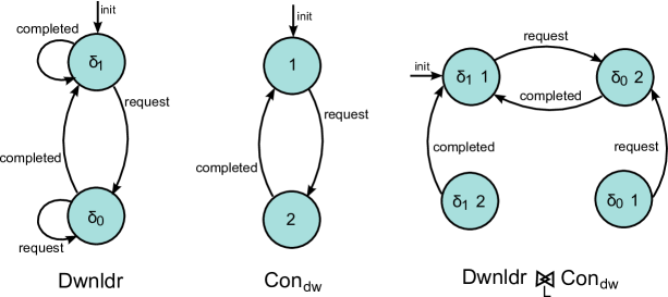
Figure 2: Schematic representation of the TDSHA $\mathcal{T}(\mathit{Dwnldr})$, associated with the download module of the Orbiter, (left) of the TDSHA $\mathcal{T}(\mathit{Con}_{\mathit{dw}})$ associated with the download controller (middle) and of their TDSHA product $\mathcal{T}(\mathit{Dwnldr})\otimes_{L}\mathcal{T}(\mathit{Con}_{\mathit{dw}})$ (right).

Consider the subcomponent

$$\mathit{Dwnldr}\stackrel{{\scriptstyle\mbox{\em{\tiny def}}}}{{=}}\text{\text@underline{init}}{\,:\,}\delta_{1}.\mathit{Dwnldr}+\overline{\text{request}}{\,:\,}\delta_{0}.\mathit{Dwnldr}+\overline{\text{completed}}{\,:\,}\delta_{1}.\mathit{Dwnldr}$$

describing the downloading module of the Orbiter system of Section 2. The TDSHA associated with it is visually depicted in Figure 2 (left). It has two modes, corresponding to the two different influences $\delta_{1}=(\mathit{dw},r,\mathit{const})$ and $\delta_{0}=(\mathit{dw},0,\mathit{const})$, and two edges, labeled by $\overline{\text{request}},\overline{\text{completed}}$. The initial state is the mode corresponding to $\delta_{1}$.

We collect now such considerations into a formal definition.

Definition 5

Let $S=\sum_{i=1}^{k}\textrm{a}_{i}{\,:\,}\alpha_{i}.S+\text{\text@underline{init}}{\,:\,}\alpha.S$ be a subcomponent of the HYPE model $(\mathit{ConSys},\mathcal{V},\mathit{IN},\mathit{IT},$ $\mathcal{E}_{d},\mathcal{E}_{s},\mathcal{A},\mathop{\mathit{ec}},\mathop{\mathit{iv}},\mathit{EC},\mathit{ID})$. The TDSHA
$\mathcal{T}(S)=(Q,\mathbf{X},\mathcal{TC},\mathcal{TD},\mathcal{TS},\mathrm{init},\mathcal{E})$ associated with $S$ is defined by

1. $Q=\{q_{\alpha}~{}|~{}\alpha\in\mathsf{is}(S)\}$; $\mathbf{X}=\mathcal{V}$; $\mathcal{E}=\mathcal{E}_{d}\cup\mathcal{E}_{s}$;

2. $\mathrm{init}=(q_{\alpha},true)$, where $S=\text{\text@underline{init}}{\,:\,}\alpha.S+S^{\prime}$;

3. $\mathcal{TC}=\{(q_{\alpha},\mathbf{1}_{\mathop{\mathit{iv}}(\mathit{i}_{S})},r\cdot\llbracket I\rrbracket)~{}|~{}\alpha=(\mathit{i}_{S},r,I)\in\mathsf{is}(S)\}$, where $\mathbf{1}_{\mathop{\mathit{iv}}(\mathit{i}_{S})}$ is the vector equal to 1 for the component corresponding to variable $\mathop{\mathit{iv}}(\mathit{i}_{S})$ and zero elsewhere;

4. $\mathcal{TD}=\{(q_{\alpha_{1}},q_{\alpha_{2}},1,true,true,\text{\text@underline{a}})~{}|~{}\text{\text@underline{a}}\in\mathsf{ev}(S)\cap\mathcal{E}_{d}\wedge\alpha_{1}\in\mathsf{is}(S)\wedge S=\text{\text@underline{a}}{\,:\,}\alpha_{2}.S+S^{\prime}\}$

5. $\mathcal{TS}=\{(q_{\alpha_{1}},q_{\alpha_{2}},true,true,\mathit{act}(\overline{\text{a}}),\overline{\text{a}})~{}|~{}\overline{\text{a}}\in\mathsf{ev}(S)\cap\mathcal{E}_{s}\wedge\alpha_{1}\in\mathsf{is}(S)\wedge S=\text{\text@underline{a}}{\,:\,}\alpha_{2}.S+S^{\prime}\}$

Once we have the TDSHA of all subcomponents, we can build the TDSHA of the full uncontrolled system by applying the product construction of TDSHA. We capture this in the following definition.

Definition 6

  

1. Let $P=P_{1}\raisebox{-4.30554pt}{$\;\stackrel{{\scriptstyle\mbox{\large$\rhd\!\!\!\!\!\lhd$}}}{{\scriptscriptstyle L}}\,$}P_{2}$ be a component. Its TDSHA is defined recursively by $\mathcal{T}(P_{1}\raisebox{-4.30554pt}{$\;\stackrel{{\scriptstyle\mbox{\large$\rhd\!\!\!\!\!\lhd$}}}{{\scriptscriptstyle L}}\,$}P_{2})=\mathcal{T}(P_{1})\otimes_{L}\mathcal{T}(P_{2})$.

2. Let $\Sigma=\Sigma_{1}\raisebox{-4.30554pt}{$\;\stackrel{{\scriptstyle\mbox{\large$\rhd\!\!\!\!\!\lhd$}}}{{\scriptscriptstyle L}}\,$}\Sigma_{2}$ be an uncontrolled system. Its TDSHA is defined recursively by $\mathcal{T}(\Sigma_{1}\raisebox{-4.30554pt}{$\;\stackrel{{\scriptstyle\mbox{\large$\rhd\!\!\!\!\!\lhd$}}}{{\scriptscriptstyle L}}\,$}\Sigma_{2})=\mathcal{T}(\Sigma_{1})\otimes_{L}\mathcal{T}(\Sigma_{2})$.

TDSHA of the controller.

Dealing with the controller is simpler, as controllers are essentially finite state automata which impose causality on the happening of events. As anticipated at the beginning of the section, event conditions will be assigned to edges of TDSHA associated with controllers. Controllers are defined by the two level syntax $M=\text{\text@underline{a}}.M\mid M+M$ and $Con=M\mid Con\raisebox{-4.30554pt}{$\;\stackrel{{\scriptstyle\mbox{\large$\rhd\!\!\!\!\!\lhd$}}}{{\scriptscriptstyle l}}\,$}Con$, hence sequential controllers are composed in parallel and synchronized on sets of actions. As for the uncontrolled system, we will first define the TDSHA of sequential controllers, and then combine them with the TDSHA product construction. Note that all events will be properly dealt with through this construction, as they all appear in the controller, see Remark 1.

Consider a sequential controller $M=\sum_{i}\textrm{a}_{i}.M_{i}$. The derivative set of $M$ is defined recursively by $ds(M)=\{M\}\cup\bigcup_{i}ds(M_{i})$, where two summations coincide if they are equal up to permutation of addends.

Definition 7

Let $(\mathit{ConSys},\mathcal{V},\mathit{IN},\mathit{IT},\mathcal{E}_{d},\mathcal{E}_{s},\mathcal{A},\mathop{\mathit{ec}},\mathop{\mathit{iv}},\mathit{EC},\mathit{ID})$ be a HYPE model with sequential controller $M$. Then $\mathcal{T}(M)=(Q,\mathbf{X},\mathcal{TC},\mathcal{TD},\mathcal{TS},\mathrm{init},\mathcal{E})$, the TDSHA associated with $M$, is defined by

1. $Q=\{q_{M^{\prime}}~{}|~{}M^{\prime}\in ds(M)\}$; $\mathbf{X}=\mathcal{V}$; $\mathcal{E}=\mathcal{E}_{d}\cup\mathcal{E}_{s}$;

2. $\mathrm{init}=(q_{M},\mathit{res}(\text{\text@underline{init}}))$, where $\mathit{res}(\text{\text@underline{init}})$ is the reset associated with the init event.

3. $\mathcal{TC}=\emptyset$;

4. $\mathcal{TD}=\{(q_{M_{1}},q_{M_{2}},1,\mathit{act}(\text{\text@underline{a}}),\mathit{res}(\text{\text@underline{a}}),\text{\text@underline{a}})~{}|~{}M_{1}=\text{\text@underline{a}}.M_{2},\ M_{1},M_{2}\in ds(M),\ \text{\text@underline{a}}\in\mathcal{E}_{d},\ \mathop{\mathit{ec}}(\text{\text@underline{a}})=(\mathit{act}(\text{\text@underline{a}}),$ $\mathit{res}(\text{\text@underline{a}}))\}$;

5. $\mathcal{TS}=\{(q_{M_{1}},q_{M_{2}},true,\mathit{res}(\overline{\text{a}}),\mathit{act}(\overline{\text{a}}),\overline{\text{a}})~{}|~{}M_{1}=\overline{\text{a}}.M_{2},\ M_{1},M_{2}\in ds(M),\ \overline{\text{a}}\in\mathcal{E}_{s},\ \mathop{\mathit{ec}}(\overline{\text{a}})=(\mathit{act}(\overline{\text{a}}),$ $\mathit{res}(\overline{\text{a}}))\}$, where $\mathit{act}(\overline{\text{a}}):\mathbb{R}^{|\mathcal{V}|}\rightarrow\mathbb{R}^{+}$ is the rate of the transition;

Definition 8

Let $Con=Con_{1}\raisebox{-4.30554pt}{$\;\stackrel{{\scriptstyle\mbox{\large$\rhd\!\!\!\!\!\lhd$}}}{{\scriptscriptstyle L}}\,$}\mathit{Con}_{2}$ be a controller. The TDSHA of $Con$ is defined recursively as $\mathcal{T}(Con)=\mathcal{T}(Con_{1})\otimes_{L}\mathcal{T}(Con_{2})$.

The product construction of Definitions 6 and 8 can be carried on because the factors TDSHA are reset-compatible and init-compatible. This is trivial both for the uncontrolled system (all resets are $true$) and for the controller (resets for the same event are equal). Furthermore, stochastic transitions have consistent rates, as their rate depends only on the labelling event.

Consider the controller of the download module of the orbiter; its TDSHA is depicted in Figure 2 (middle), omitting the explicit representation of rates and resets.

TDSHA of the HYPE model.

Once we have built the TDSHA of the controller and of the uncontrolled system, we simply have to take their product.

Definition 9

Let $(\mathit{ConSys},\mathcal{V},\mathit{IN},\mathit{IT},\mathcal{E}_{c},\mathcal{E}_{s},\mathcal{A},\mathop{\mathit{ec}},\mathop{\mathit{iv}},\mathit{EC},\mathit{ID})$ be a HYPE model, with controlled system $\mathit{ConSys}=\Sigma\raisebox{-4.30554pt}{$\;\stackrel{{\scriptstyle\mbox{\large$\rhd\!\!\!\!\!\lhd$}}}{{\scriptscriptstyle L}}\,$}\text{\text@underline{init}}.\mathit{Con}$. The TDSHA associated with $\mathcal{M}$ is

$$\mathcal{T}(\mathcal{M})=\mathcal{T}(\Sigma)\otimes_{L}\mathcal{T}(\mathit{Con}).$$

Example 1

In Figure 2 (right) we show the product $\mathcal{T}(Dwnldr)\otimes_{L}\mathcal{T}(\mathit{Con}_{\mathit{dw}})$, $L=\{\overline{\text{request}},\overline{\text{completed}}\}$, in order to give an idea of the product construction. In Figure 3, instead, we show a trajectory of the variable $D$, describing the amount of data collected. As we can see, periods in which the data is collected (linearly), are interleaved by downloads, in which data is not accumulated. Once the download has finished, $D$ is set back to zero. Both the download time and the periods between two consecutive downloads are randomly distributed.

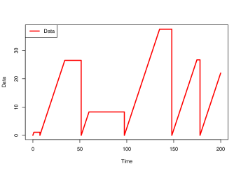
Figure 3: Sampled trajectory of the accumulated data of the extended orbiter model of Section 2.1. Data increases during accumulation phases, and remains constant during downloads. It is erased right after the download finished. Rate values, fixed just for illustrative purposes, are $r=1.0$, $\lambda_{r}=0.04$, $\lambda=0.5$, $\mu=10.0$.

As already evident from the previous example, the construction we have defined actually generates TDSHA with many unreachable states. This is a consequence of the fact that sequentiality and causality on actions is imposed just on the final step, when the controller is synchronized with the uncontrolled system. Once the TDSHA is constructed, however, it can be pruned by removing unreachable states (the TDSHA of Figure 2 (right) has indeed just two reachable states from the initial one). In order to limit combinatorial explosion, one can prune TDSHA’s at each intermediate stage. A formal definition of this policy, however, would have made the mapping from HYPE to TDSHA much more complex.

Orbiter revisited.

We consider now a more complex version of the orbiter, in which the download time depends also on the current temperature. The operational speed of the download can be reduced linearly down to zero if the temperature is too high or too low. In order to implement such a modification, we simply have to modify the rate function in the event condition of event $\overline{\text{completed}}$, replacing it with a suitable function of accumulated data and temperature. A sampled trajectory is shown in Figure 4 (left), while in Figure 4 (right) we show how the firing time of $\overline{\text{completed}}$ depends on temperature.

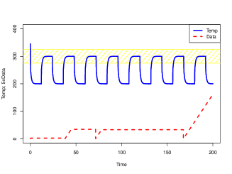
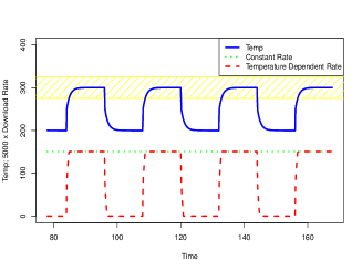
Figure 4: (left) Sampled trajectory of the accumulated data of the extended orbiter model of Section 2.1, with download rate depending on temperature. The rate is maximal, and equal to $\frac{\lambda}{\mu+D}$ when temperature is in the operational regime, in this example, when $275\leq K\leq 325$. When the temperature is lower than 275 (higher than 325), the download rate linearly decreases to 0, reaching it when $K=225$ ($K=350$). Rate values, for the downloader are $r=1.0$, $\lambda_{r}=0.1$, $\lambda=1.0$, $\mu=10.0$. Rates and parameters for the temperature control mechanism are $f_{h}=200$, $r_{d}=100$, $r_{s}=400$, $k_{1}=k_{2}=250$, $k_{3}=k_{4}=300$. The download time becomes longer with respect to Figure 3, as the temperature falls repeatedly below the operational regime. (right) Plot of the downloading rate when it is constant (green) or when it depends on temperature (red). In the latter case, the rate is periodically reduced to zero, as temperature falls below 225. The shadowed region indicates, in both plots, the interval of temperatures in which the download has maximum speed.

5 Related Work

The modelling approach of HYPE, based on the composition of individual flows, makes it different from other hybrid process algebras [12] and from hybrid automata [9]. In these other approaches the continuous dynamics is specified by embedding ODEs within the syntactic description of models, while in HYPE, ODEs emerge as a combination of active flows. A more detailed comparison between HYPE and other hybrid modelling formalisms can be found in [7, 8].

As far as stochastic hybrid systems are concerned, there has been previous work aimed at making modelling compositional. In [13], Strubbe et al. introduce Communicating Piecewise Deterministic Markov Processes (CPDP). This is an automata based formalism which models a system as interacting automata. Their chosen level of abstraction is somewhat lower level than ours, comparable with TDSHA. In CPDP, as in HYPE, instantaneous transitions may be triggered either by conditions of the continuous variables (boundary-hit transitions) or by the expiration of a stochastic determined delay (Markov transitions). Interaction between automata is based on one-way synchronisation: in each interaction one partner is active while the other is passive. In HYPE, instead, all components may be regarded as active with respect to each transition in which they participate, as activation conditions are specified uniquely in the model. Components participating in a discrete transition are determined by the construction of the HYPE model, where the synchronisation set $L$ in $\;\stackrel{{\scriptstyle\mbox{\large$\rhd\!\!\!\!\!\lhd$}}}{{\scriptscriptstyle L}}\,$ specifies which actions must be shared.

The synchronization mechanics of CPDP has been extended in [14], introducing an operator which exploits all possible interactions of active and passive actions. In [15] the authors define a notion of bisimulation for both PDMPs and CPDPs and show that if CPDPs are bisimilar then they give rise to bisimilar PDMPs. Furthermore the equivalence relation is a congruence with respect to the composition operator of CPDPs.

6 Conclusions

In this paper we extended the hybrid process algebra HYPE, allowing events to fire at (exponentially distributed) random times. Although from a syntactic point of view the modifications with respect to the original version of HYPE are minimal (non-urgent events become stochastic by replacing their activation condition $\bot$ with a functional rate), the semantics of the language is considerably enriched. The stochastic hybrid systems obtained from HYPE models fall in the class of Piecewise Deterministic Markov Processes. In the paper, we concentrated on showing how such a semantics can be defined. We used an intermediate formalism, namely Transition-Driven Stochastic Hybrid Automata, which can then be mapped to PDMPs. The way we defined the semantics in terms of TDSHA is quite different from the original definition of [7, 8], in which a hybrid automaton is extracted from the labeled transition system of a HYPE model, defined according to a suitable operational semantics. Here, instead, we directly manipulate the model at the syntactic level.

The mapping from TDSHA to PDMP is quite straightforward, except in one point: One has to check that the HYPE model is well-behaved, meaning that it is not possible that an infinite sequence of instantaneous transitions fires in the same time instant. Unfortunately, checking this property in general is undecidable, hence in [8] we put forward a set of decidable but stricter conditions on HYPE models, that guarantee that a model is well-behaved and that are usually satisfied in practical cases.

As the syntax of HYPE is basically unchanged, all the results of [7, 8] depending on syntactic features still hold. In particular, the notion of bisimulation of HYPE models extends untouched in this new setting. As a future investigation, we plan to compare this bisimulation relation with other bisimulations designed for PDMPs [15].

In the current version of HYPE, stochasticity has been introduced just in terms of random occurrence in the time of events. It is often useful to have stochasticity also in resets. This would allow the quantitative modelling of uncertainty in the outcome of certain actions. Such an extension can be done along the lines of the current paper, even if it requires a modification of the definition of TDSHA, allowing stochastic resets. However, the class of target stochastic processes remains that of PDMP.

Future work includes also the implementation of an efficient simulator for (stochastic) HYPE. Moreover, we will model specific case studies, to prove its effectiveness as a hybrid modelling language.

Acknowledgements  

This work was supported by Royal Society International Joint Project (JP090562). Vashti Galpin is supported by the EPSRC SIGNAL Project, Grant EP/E031439/1. Luca Bortolussi is supported by GNCS. Jane Hillston has been supported by EPSRC under ARF EP/c543696/01.

References

- [1] L. Bortolussi, V. Galpin, J. Hillston, and M. Tribastone. Hybrid Semantics for PEPA. In Proc. of QEST 2010, pp. 181–190. 10.1109/QEST.2010.31
- [2] L. Bortolussi and A. Policriti. Hybrid Semantics of Stochastic Programs with Dynamic Reconfiguration. In Proc. of CompMod 2009, EPTCS 6, 2009, pp. 63–76. 10.4204/EPTCS.6.5
- [3] F. Ciocchetta and J. Hillston. Bio-PEPA: A framework for the modelling and analysis of biological systems. Theoretical Computer Science, 410:3065-3084, 2009. 10.1016/j.tcs.2009.02.037
- [4] M.H.A. Davis. Markov Models and Optimization. Chapman & Hall, 1993.
- [5] M. B. Elowitz and S. Leibler. A synthetic oscillatory network of transcriptional regulators. Nature, 403:335–338, 2000. 10.1038/35002125
- [6] V. Galpin, J. Hillston, and L. Bortolussi. HYPE applied to the modelling of hybrid biological systems. Electronic Notes in Theoretical Computer Science, 218:33–51, 2008. 10.1016/j.entcs.2008.10.004
- [7] V. Galpin, J. Hillston, and L. Bortolussi. HYPE: a process algebra for compositional flows and emergent behaviour. In: Proc. of CONCUR 2009, Lecture Notes in Computer Science, LNCS 5710, pp. 305–320. 10.1007/978-3-642-04081-8_21
- [8] V. Galpin, J. Hillston, and L. Bortolussi. HYPE: hybrid modelling by composition of flows. Journal version, submitted for publication.
- [9] T. A. Henzinger. The theory of hybrid automata. In Proc. of LICS 1996, pages 278–292.
- [10] J. Hillston. Fluid flow approximation of PEPA models. In Proc. of QEST 2005, pp 33–43. 10.1109/QEST.2005.12
- [11] J. Hillston. A Compositional Approach To Performance Modelling. CUP, 1996.
- [12] U. Khadim. A comparative study of process algebras for hybrid systems. Computer Science Report 06-23, Technische Universiteit Eindhoven, 2006. http://alexandria.tue.nl/extra1/wskrap/publichtml/200623.pdf.
- [13] S.N. Strubbe, A.A. Julius and A.J. van der Schaft. Communicating Piecewise Deterministic Markov Processes. In Proc. of ADHS 2003, 349-354.
- [14] S.N. Strubbe and A.J. van der Schaft. Stochastic semantics for Communicating Piecewise Deterministic Markov Processes. In Proc. of IEEE CDC 2005, pp. 6103–6108. 10.1109/CDC.2005.1583138
- [15] S.N. Strubbe and A.J. van der Schaft. Bisimulation for Communicating Piecewise Deterministic Markov Processes. In Proc. of HSCC 2005, LNCS 3414. 10.1007/b106766
- [16] M. Tribastone, S. Gilmore and J. Hillston, Scalable differential analysis of process algebra models. IEEE Transactions on Software Engineering, 2010, to appear. 10.1109/TSE.2010.82
- [17] B. Tuffin, D. S. Chen, and K. S. Trivedi. Comparison of hybrid systems and fluid stochastic Petri nets. Discrete Event Dynamic Systems: Theory and Applications, 11:77–95, 2001. 10.1023/A:1008387132533