Two-Player Reachability-Price Games on Single-Clock Timed Automata

Abstract

We study two player reachability-price games on single-clock timed automata. The problem is as follows: given a state of the automaton, determine whether the first player can guarantee reaching one of the designated goal locations. If a goal location can be reached then we also want to compute the optimum price of doing so. Our contribution is twofold. First, we develop a theory of cost functions, which provide a comprehensive methodology for the analysis of this problem. This theory allows us to establish our second contribution, an EXPTIME algorithm for computing the optimum reachability price, which improves the existing 3EXPTIME upper bound.

1 Introduction

Timed automata [2] are a formalism used for modeling real time systems, i.e., systems whose behavior depends on time. Timed automata are finite automata augmented with a set of clocks. The values of the clocks grow uniformly over time. There are two types of transitions: continuous, resulting in time progression, and discrete, resulting in a change of location. Discrete transitions may reset values of certain clocks to zero, and different transitions may be enabled at different clock values.

Optimal schedule synthesis is one of the key areas of research in timed automata theory [8, 9, 10, 12, 13]. In this setting, timed automata are augmented with pricing information, and each execution of the automaton is assigned a payoff. Moreover, we want to model lack of full control over the system; game theory is commonly used in this context [6, 10, 11, 13, 12]. There are two players: the minimizer and the maximizer, who have opposite goals of minimizing and maximizing the payoff of a play, respectively. In this case a play is an execution of the automaton, and we are dealing with the worst case scenario, where the controller is interacting with an adversarial environment. In this context, reachability-price games are commonly considered [7, 10, 12]. In these games the goal is to optimize the accumulated price of reaching a designated set of states.

When the payoff of an execution is simply its time duration, synthesizing an almost-optimal schedule is EXPTIME-complete [12]. In linearly priced timed automata [7, 10], the price of an individual continuous transition is its duration multiplied by a location specific price rate. Bouyer et al. show that determining the existence of an optimal schedule for linearly priced timed automata, with at least three clocks is undecidable [7]. On the other hand, Bouyer et al. show a triply exponential algorithm for single-clock linearly priced timed automata [10]. However, the exact complexity of the problem is still unknown, as PTIME is the best lower bound that is currently known.

Contributions.

In this paper, we present a new EXPTIME algorithm for optimal schedule synthesis for linearly priced single-clock timed automata with non-negative price rates. Our work improves the triply exponential algorithm given by Bouyer et al. [10].

Our contribution is twofold. First, in order to deliver the main result, we establish technical results regarding cost functions, i.e., piecewise affine continuous functions that are non-increasing. Cost functions in this form were first considered by Bouyer et al. [10]. They are central to both algorithms, the one presented in this paper, and that of Bouyer et al. [10], as both algorithms use them to produce their output. The output of the algorithms is a function that assigns the optimal price of reachability to each state; this output function can be represented by a finite set of cost functions. Our technical results regard operations performed on cost functions during the execution of the algorithm. We establish the properties and invariants of these operations, which later allows us to analyze the complexity, and prove the correctness of the algorithm. This understanding of cost functions was pivotal in achieving the doubly-exponential speedup, and we believe that this detailed analysis might prove useful in further closing the existing complexity gap.

Second, we show an EXPTIME algorithm for computing the optimal price of reachability. As in Bouyer’s et al. approach [10], the algorithm does the computation through a recursive procedure, with respect to the number of locations of the timed automaton. Again, as in Bouyer’s et al. work [10], in each recursive call we single out the location that minimizes the price rate. In the model, locations are assigned to players, which necessitates different handling of a location, depending on its ownership. In the case of the maximizer locations, our algorithm behaves exactly like the original, however, when it comes to handling minimizer locations, we improve over the predecessor. The original algorithm would proceed to recursively solve two subproblems, which resulted in an additional exponential blowup. The algorithm presented in this paper, as in the case of maximizer locations, employs an iterative procedure which prevents this blowup. The approach is similar in spirit to that used in handling maximizer locations, however, the details are different.

Tools for handling games, where the price of an execution is its time duration, already exist (e.g., UPPAAL [3]). We believe that the work presented in this paper may help in the development of such tools for reachability-price games on linearly priced timed automata.

2 Preliminaries

Cost functions.

Below we introduce the notion of a cost function, and prove some of its basic properties. Cost functions are a central notion when considering reachability-price games on single-clock timed automata. The theory of cost functions will be used to construct the algorithm for computing the optimal reachability cost, as well as to prove its correctness.

In this paper, we will be dealing with the ordered set of real numbers augmented with the greatest element, positive infinity. For that purpose we need to extend the $+$, $\min$ and $\max$ operators in a natural way. For $a\in\mathbb{R}\cup\{\infty\}$ we have $a+\infty=\infty$, $\max(a,\infty)=\infty$ and $\min(a,\infty)=a$.

Definition 1 (Cost function)

A function $f:I\to\mathbb{R}\cup\{\infty\}$ that is continuous, non-increasing, and piecewise affine, where $I$ is a bounded interval, is said to be a cost function. We will write $\mathcal{CF}(I)\subseteq[I\to\mathbb{R}\cup\{\infty\}]$ to denote the set of all cost functions with the domain $I$.

Remark 2

Notice that if $f\in\mathcal{CF}(I)$, and $f(x)=\infty$ for some $x\in I$ then $f\equiv\infty$, over $I$. $\square$

At times, we will need to talk about the individual affine functions, i.e., the pieces of a cost function. To make this easier, we introduce the following convention. Given an interval $I$, let $f:I\to\mathbb{R}$ be a cost function, we will write $f=\langle f_{1},\ldots,f_{k}\rangle$ to denote the fact that the piecewise affine function $f$ consists of affine pieces $f_{1},\ldots,f_{k}$, with domains $I_{1},\ldots,I_{k}$, where $k$ is the smallest integer such that

$$f(x)=\begin{cases}f_{1}(x)&x\in I^{f}_{1}\\ \lx@intercol\hfil\dotsb\hfil\lx@intercol\\ f_{k}(x)&x\in I^{f}_{k}.\end{cases}$$

Throughout the paper, we will be implicitly assuming that $I=[b,e]$, and that $I^{f}_{i}=\left[b_{i}^{f},e_{i}^{f}\right]$, for $i\in\{1,\ldots,k\}$, with $e_{i+1}^{f}=b_{i}^{f}$, for $i\in\{1,\ldots,k-1\}$. The formula for the individual segment $f_{i}$ will be given by $a^{f}_{i}\cdot x+c^{f}_{i}$, for $i\in\{1,\ldots,k\}$. If $f$ is clear from the context, we will omit the superscript.

We now introduce two operators, which are key in defining the relationship between reachability cost functions of a location and its successors. This will be later summarized by Lemma 13. Given a cost function $f:[b,e]\to\mathbb{R}\cup\{\infty\}$ and a positive constant $c$, we define the following two operators, that transform cost functions:

$$\operatorname{minC}(f,c)=x\mapsto\min_{0\leqslant t\leqslant e-x}ct+f(x+t)$$

and $\operatorname{maxC}(f,c)$ defined analogously, with max substituted for min.

Lemma 3

Let $c$ be a positive constant. If $f:[b,e]\to\mathbb{R}$ is a cost function then $\operatorname{minC}(f,c)$ is a cost functions as well. The same holds for $\operatorname{maxC}$.

The following Proposition formalizes the intuition how the $\operatorname{minC}$ ($\operatorname{maxC}$) operators affect the function $f$. The $\operatorname{minC}$ ($\operatorname{maxC}$) operator removes all pieces of $f$ that have slopes steeper (shallower) than $-c$, and substitutes them with pieces that have a slope equal to $-c$. For the remaining pieces, the formula remains unchanged, but the domain may change. However, the new domain is always a subset of the domain in $f$.

Proposition 4

Let $f=\langle f_{1},\ldots,f_{k}\rangle$ and let $\operatorname{minC}(f,c)=\langle g_{1},\ldots,g_{l}\rangle$. We have that $l\leqslant k$, and for every $j\leqslant l$: if the formulas for $g_{j}$ and $f_{i}$ are equal, for some $i\leqslant k$, then $b^{f}_{i}\in I^{g}_{j}\subseteq I^{f}_{i}$, otherwise $a^{g}_{j}>-c$. Moreover, $a^{g}_{j}\geqslant-c$, for all $j=1,\ldots,l$.

For $\operatorname{maxC}$ we can prove a similar result, with the only difference that in the statement of Prop. 4 $<$ and $\leqslant$ are substituted for $>$ and $\geqslant$.

Example 5

Fig. 1 gives an intuitive understanding of the $\operatorname{minC}(f,c)$ operator, for a cost function $f$ and a positive real constant $c$. The cost function is given as $f=\langle f_{1},\ldots,f_{7}\rangle$ (as seen in Fig. 1 a)). The slope of $f_{2}$ and $f_{6}$ is smaller than $-c$; for the remaining components it is greater. The cost function $g=\operatorname{minC}(f,c)$ is depicted in Fig. 1 b), and is given by $\langle g_{1},\ldots,g_{6}\rangle$. All components of $g$ have a slope greater or equal to $-c$. The formula for $g_{1}$ is the same as for $f_{1}$, however, the domain is a subset (similarly for $f_{4}$ and $g_{4}$). The function $g_{3}$ is equal to $f_{3}$ (similarly $g_{6}$ is equal to $f_{7}$). Functions $g_{2}$ and $g_{5}$, have the slope $-c$, and where not present in $f$. $\square$

a)		b)

Figure 1: a) Cost function $f$, before applying $\operatorname{minC}(f,c)$ operator — dashed lines have a slope $-c$; b) cost function $g=\operatorname{minC}(f,c)$ — dashed lines denote parts of $f$ that do not coincide with $g$.

Reachability-price games.

A reachability-price game is played on a transition system whose states are partitioned between two players, the minimizer and the maximizer. A game starts in some state, and the players change the current state according to the transition rules, with the owner of the state deciding which transition to take. The goal of the minimizer is to reach a state in the designated set of goal states, whereas the goal of the maximizer is to prevent this from happening. Each transition incurs a price, and the minimizer, if she can assure that a goal state is reached, wants to minimise the total price of doing so. If the maximizer cannot prevent the minimizer from reaching a goal state, then his goal is to maximise the total price of reaching one.

A weighted labeled transition system, or simply a transition system, $\mathcal{T}=\langle S,\Lambda,\xrightarrow{},\pi\rangle$, consists of a set of states, $S$, a set of labels, $\Lambda$, a labeled transition relation $\xrightarrow{}\;\subseteq S\times\Lambda\times S$, and a price function $\pi$ that assigns a real number to every transition. We will write $s\xrightarrow{\lambda}s^{\prime}$ to denote a transition, i.e., an element $(s,\lambda,s^{\prime})\in\;\xrightarrow{}$. We will say that the transition system is deterministic, if the relation $\xrightarrow{}$ can be viewed as a function $\xrightarrow{}\;:S\times\Lambda\to S$.

Remark 6

For the remainder of the paper we will be considering deterministic weighted labeled transition systems. $\square$

Weighted transition systems will be used to provide the semantics for single-clock timed automata, considered in this paper. In this context, the restriction made in Rem. 6 is not constraining, as single-clock timed automata yield deterministic transition systems. We place this restriction because it allows for simpler definitions (e.g., we rely on this restriction when defining the notion of a run induced by the players strategies).

A reachability-price game $\Gamma=\langle\mathcal{T},S^{\mathrm{Min}},S^{\mathrm{Max}},S^{\mathrm{Goal}},f^{\mathrm{Goal}}\rangle$ consists of a weighted transition labeled system, $\mathcal{T}$, a partition of the transition system’s set of states, into the minimizer and maximizer states, $S^{\mathrm{Max}}=S\setminus S^{\mathrm{Min}}$, a designated set of goal states, $S^{\mathrm{Goal}}\subseteq S$, and goal cost function, $f^{\mathrm{Goal}}:S^{\mathrm{Goal}}\to\mathbb{R}$.

Given a state $s$, a run of the game from $s$ is a (possibly infinite) sequence of transitions $\omega=s_{0}\xrightarrow{\lambda_{1}}s_{1}\xrightarrow{\lambda_{2}}s_{2}\cdots$, where $s=s_{0}$. If two runs $\omega=s_{0}\xrightarrow{\lambda_{1}}\cdots\xrightarrow{\lambda_{k}}s_{k}$ and $\omega^{\prime}=s_{0}^{\prime}\xrightarrow{\lambda_{1}}\cdots$ are such that $s_{k}=s_{0}^{\prime}$ then, $\omega\omega^{\prime}$ denotes the run $s_{0}\xrightarrow{\lambda_{1}}\cdots\xrightarrow{\lambda_{k}}s_{k}\xrightarrow{\lambda_{1}^{\prime}}\cdots$. Given a finite run $\omega$, $mathrm{Len}(\omega)$ will denote its length, i.e., the total number of transitions, $mathrm{Last}(\omega)$ will denote the final state of $\omega$, i.e., $s_{mathrm{Len}(\omega)}$, and $\omega_{n}$ will denote the prefix of $\omega$ of length $n$, where $n\leqslant mathrm{Len}(\omega)$. The set of all runs of $\Gamma$ is denoted by $\mathrm{Runs}$. The set of all finite runs of $\Gamma$ is denoted by $\mathrm{Runs}_{\mathrm{fin}}$. Note that $\mathrm{Runs}_{\mathrm{fin}}\subseteq\mathrm{Runs}$. We will also write $\mathrm{Runs}(s)$ ($\mathrm{Runs}_{\mathrm{fin}}(s)$) to denote the set of all runs (all finite runs) starting in a state $s$.

A strategy of the minimizer is a partial function $\mu:\mathrm{Runs}_{\mathrm{fin}}\to\Lambda$ such that for every finite run $\omega$, ending in a state of the minimizer, $Last(\omega)\xrightarrow{\mu(\omega)}s^{\prime}$. We will say that $\mu$ is positional if it can be treated as a function $\mu:S\to\Lambda$. We will write $\Sigma^{\mathrm{Min}}$ and $\Pi^{\mathrm{Min}}$ to denote the sets of all and all positional strategies of the minimizer, respectively. The set of strategies for the maximizer is defined analogously.

Given a run $\omega^{\prime}$ ending in a state $s_{0}$, and a pair of strategies $\sigma\in\Sigma^{\mathrm{Min}}$ and $\chi\in\Sigma^{\mathrm{Max}}$, we write $\mathrm{Run}(\omega^{\prime},\mu,\chi)$ to denote the unique run $\omega\in\mathrm{Runs}(s_{0})$ satisfying: if $s_{i}\xrightarrow{\lambda_{i+1}}s_{i+1}$ is the $(i+1)$-th transition, of $\omega$, then $\mu(\omega^{\prime}\omega_{i})=\lambda_{i}$ if $s_{i}\in S^{\mathrm{Min}}$, otherwise, $\chi(\omega^{\prime}\omega_{i})=\lambda_{i}$. Note that, if $\mu$ and $\chi$ are positional, then $\omega^{\prime}$ is irrelevant.

Given a finite run $\omega$ we define its price, $\mathrm{Price}(\omega)$, as $\sum_{i=1}^{mathrm{Len}(\omega)}\pi((s_{i-1},\lambda_{i},s_{i}))$, i.e., the total price of its transitions. Given a run $\omega\in\mathrm{Runs}$, let $\mathrm{Stop}(\omega)=\min\{i\>:\>s_{i}\in S^{\mathrm{Goal}}\}$. The cost of a run $\omega$ is defined as:

$$\mathrm{Cost}(\omega)=\begin{cases}f^{\mathrm{Goal}}(mathrm{Last}(\omega_{\mathrm{Stop}(\omega)}))+\mathrm{Price}(\omega_{\mathrm{Stop}(\omega)})&\mathrm{Stop}(\omega)<\infty,\\ \infty&\text{ otherwise.}\end{cases}$$

We now define the function $\mathrm{OptCost}:S\to\mathbb{R}\cup\{\infty\}$, which maps every state to the minimum cost of reaching a goal state that can be guaranteed by the minimizer. If the maximizer can prevent the minimizer from achieving a goal state, the cost is $\infty$. The function is defined as:

$$\mathrm{OptCost}(s)=\inf_{\mu\in\Sigma^{\mathrm{Min}}}\sup_{\chi\in\Sigma^{\mathrm{Max}}}\mathrm{Cost}(\mathrm{Run}(s,\mu,\chi)).$$

Finally, we introduce the notion of $\varepsilon$-optimality, for $\varepsilon>0$. We say that $\mu\in\Sigma^{\mathrm{Min}}$ is $\varepsilon$-optimal, if $\sup_{\chi\in\Sigma^{\mathrm{Max}}}\mathrm{Cost}(\mathrm{Run}(\omega,\mu,\chi))\leqslant\mathrm{OptCost}(mathrm{Last}(\omega))+\varepsilon$ for all $\omega\in\mathrm{Runs}_{\mathrm{fin}}$. Given a strategy $\mu\in\Sigma^{\mathrm{Min}}$ we say that $\chi\in\Sigma^{\mathrm{Max}}$ is $\varepsilon$-optimal for $\mu$, if $\mathrm{Cost}(\mathrm{Run}(\omega,\mu,\chi))\geqslant\mathrm{OptCost}(mathrm{Last}(\omega))-\varepsilon$, for all $\omega\in\mathrm{Runs}_{\mathrm{fin}}$.

The decision problem associated with reachability-price games is the following:

Problem 7

Given a reachability-price game $\Gamma$, its state $s$, and a real constant $c$, determine whether $\mathrm{OptCost}(s)\leqslant c$. $\square$

If $\mathcal{T}$ or $\Gamma$ are not clear from the context we will write $\mathrm{OptCost}_{\Gamma}$, $\mathrm{Runs}_{\Gamma}$, etc.

Single-clock timed automata.

In this paper we are considering timed automata with a single clock. We write $X=\{x\}$ to denote the set containing the single clock $x$. A clock constraint is given by a closed interval with non-negative integer end points. We write $\mathcal{B}(X)$ to denote the set of all clock constraints. A clock valuation is a function that assigns a non-negative real value to the clock $x$; $\mathcal{V}=[X\to\mathbb{R}_{\geqslant 0}]$ denotes the set of all single clock valuations. A clock valuation $v$ satisfies a clock constraint $g\in\mathcal{B}(X)$ if $v(x)\in g$, and this will be denoted by $v\models g$. We write $v_{0}$ to denote the $x\mapsto 0$ valuation. For a valuation $v$ and $t\in\mathbb{R}_{\geqslant 0}$ the valuation $v+t$ denotes the valuation $x\mapsto v(x)+t$.

A weighted single-clock timed automaton $\mathcal{A}=\langle L,E,\eta,mathrm{urg},\pi\rangle$ consists of a finite set of locations, $L$, an edge relation, $E\subseteq L\times\mathcal{B}(X)\times 2^{X}\times L$, an invariant specification, $\eta:L\to\mathcal{B}(X)$, an urgency mapping, $mathrm{urg}:L\to\{0,1\}$, and weight function, $\pi:L\cup E\to{\rm Nature}$.

We assume (without loss of generality [4]) that $\mathcal{A}$ is clock-bounded, i.e., there exists a positive constant $M$ such that $v\models\eta(l)$ implies $v(x)\leqslant M$, for every location $l$.

The size of the automaton, denoted by $|\mathcal{A}|$, is the total number of bits needed to represent all of its components — constants are encoded in binary.

The semantics of a timed automaton $\mathcal{A}$ is given in terms of a deterministic weighted labeled transition system $\mathcal{T}_{\mathcal{A}}=\langle S_{\mathcal{A}},\Lambda_{\mathcal{A}},\xrightarrow{}_{\mathcal{A}},\pi_{\mathcal{A}}\rangle$. The set of states $S_{\mathcal{A}}\subseteq L\times\mathcal{V}$ is such that $v\models\eta(l)$ for every $(l,v)\in S_{\mathcal{A}}$. The set of labels is given by $\Lambda_{\mathcal{A}}=E\cup\mathbb{R}_{>0}$. The transition relation, $\xrightarrow{}_{\mathcal{A}}$ admits a transition $(l,v)\xrightarrow{\lambda}(l^{\prime},v^{\prime})$ iff one of the following is true:

Discrete transition

$\lambda=(l,g,Z,l^{\prime})\in E$, $v\models g$, and if $Z=\emptyset$ then $v=v^{\prime}$, otherwise $v^{\prime}=v_{0}$.

Continuous transition

$\lambda=t\in\mathbb{R}_{>0}$, $mathrm{urg}(l)=0$, i.e., the location is non-urgent, for every $t^{\prime}\in(0,t)$ we have $v+t^{\prime}\models\eta(l)$, $l=l^{\prime}$, and $v^{\prime}=v+t$.

Finally, the price function, $\pi_{\mathcal{A}}((l,v)\xrightarrow{\lambda}(l^{\prime},v^{\prime}))$ is defined as $\pi(\lambda)$ if $\lambda\in E$, and $\pi(l)\cdot\lambda$, otherwise.

We will often abuse notation, and treat the state of the automaton as an element of $L\times\mathbb{R}_{\geqslant 0}$, and the clock valuation as a real variable.

Remark 8

We only allow runs that do not admit infinitely many consecutive continuous transitions. Note that this requirement does not exclude Zeno runs, i.e., infinite runs whose total duration is finite. $\square$

Reachability-price games on single-clock timed automata.

Fix a partition of the set of locations, $L=L^{\mathrm{Min}}\setminus L^{\mathrm{Max}}$, into the minimizer and maximizer locations, the set of goal locations $L^{\mathrm{Goal}}\subseteq L$, and a function that assigns a cost function to every goal location, ${mathrm{CF}^{\mathrm{Goal}}}:L^{\mathrm{Goal}}\to\mathcal{CF}([0,M])$, where $M$ is the clock bound. We can define a reachability-price game on a single-clock timed automaton $\mathcal{A}$, by defining a reachability-price game on its transition system $\mathcal{T}_{\mathcal{A}}$. The reachability-price game $\Gamma_{\mathcal{A}}$ is given by $\langle\mathcal{T}_{\mathcal{A}},S^{\mathrm{Min}},S^{\mathrm{Max}},S^{\mathrm{Goal}},f^{\mathrm{Goal}}\rangle$, where: $S^{\mathrm{Min}}=S\cap(L^{\mathrm{Min}}\times\mathcal{V})$, $S^{\mathrm{Max}}=S\setminus S^{\mathrm{Min}}$, $S^{\mathrm{Goal}}=S\cap(L^{\mathrm{Goal}}\times\mathcal{V})$, and $f^{\mathrm{Goal}}((l,x))={mathrm{CF}^{\mathrm{Goal}}}(l)(x)$ for every state $(l,x)\in S^{\mathrm{Goal}}$.

The size of the game, denoted by $|\Gamma|$, is the total number of bits needed to represent all of its components — constants are encoded in binary.

Assumptions.

We are going to place some restrictions on the structure of timed automata, which will allow us to concentrate on the essence of the problem. In their work, Bouyer et al. place the same restrictions, and argue that this is without loss of generality [10]. In particular, their complexity results is stated only for the restricted automata.

Consider an interval $I$, we will write $\mathcal{A}_{I}$, for some $I$-bounded timed automaton, i.e., an automaton whose transition system has the state space restricted to $L\times I$, and for every $l$, the invariant is $\eta(l)\cap I$. To obtain the classical automaton we need to take $I=[0,\infty]$.

We say that an automaton $\mathcal{A}$ is simple if it is $[0,1]$-bounded and for every discrete transition of its transition system, the reseting set is empty, i.e., for every $e=(l,g,Z,l^{\prime})\in E$ we have $Z=\emptyset$. Notice that in simple timed-automata time always progresses.

We have the following result regarding simple single-clock timed automata.

Theorem 9

Problem 7 for reachability-price games on single-clock timed automata is polynomially Turing reducible to the analogous problem on simple single-clock timed automata.

We simplify the automaton further, by assuming that the price of every discrete transition is $0$. This assumption allows for a clearer exposition, and is without loss of generality [10]. A technique similar to that used to remove the resets can be employed. For simplicity, let $c\in{\rm Nature}$ be the constant used in Problem 7. For every state $s$, we need to consider at most $c$ copies of the slightly modified game $\Gamma$, which is played on a simple automaton with no prices on discrete transitions. Intuitively, the $\mathrm{OptCost}$ function for the $i$-th copy, gives the optimal cost of reaching goal, provided that at most $i$ transitions with non-zero prices were executed. The $\mathrm{OptCost}$ function computed for the $i$-th copy is used to construct the $(i+1)$-th copy. Each copy is treated independently, and although we might have to consider exponentially many, this does not increase the complexity as our algorithm is in EXPTIME.

Simple timed automata admit three possible edge guards, namely $[0,0]$, $[1,1]$, and $[0,1]$ (recall that we are considering only closed intervals as clock constraints). The first kind does not allow for a continuous transition, prior to a discrete one, and it is satisfied only by finitely many states. As it will be visible in the proofs of Sec. 3, the value of the $\mathrm{OptCost}$ function for such states, due to the time progression property of simple timed automata, does not “affect” the values for the other states. Transitions with guards of this kind can be dealt with, in polynomial time, during post-processing. The effect of a discrete transition, featuring a guard of the second kind, can be encoded using additional goal cost functions. Once again, proofs in Sec. 3 explain how this can be done. It is only the third kind of guards that cannot be dealt with by such simple means. In light of this, and to simplify the presentation, we assume that all transition guards are true. A similar approach was used in the work of Bouyer et al. [10].

Remark 10

In the light of the assumptions made, it is natural to think of $E$ as a subset of $L\times L$. $\square$

We will also assume that from every state the cost of reaching a goal state is finite. In light of Rem 10, one can determine the set of states, from which the maximizer can prevent reaching goal, by determining the appropriate set of locations; this can be done in polynomial time. The real complexity lies in determining the optimal cost of reaching a goal state, given that the minimizer can ensure it.

Operations.

We will now define some simple algebraic operations that we will be performing on cost functions, and reachability-price games on simple timed automata. These operations will be used in the algorithm, presented in Sec. 3.

Given two functions $h:I_{1}\to\mathbb{R}$ and $g:I_{2}\to\mathbb{R}$, we will write $f\operatorname{\triangleright}g$ to denote the override operation on these two functions [5], defined as $(h\operatorname{\triangleright}g)(x)=h(x)$ if $x\in I_{1}$ and $g(x)$ if $x\in I_{2}\setminus I_{1}$.

Fix an interval $I\subseteq[0,1]$, an automaton $\mathcal{A}$, and a reachability-price game $\Gamma$, on $\mathcal{A}$. Below we list three operations, that given a game $\Gamma$, produce a new game:

$\Gamma[mathrm{urg}(l):=1]$ denotes the game $\Gamma^{\prime}$ obtained from $\Gamma$ by changing the urgency mapping of $\mathcal{A}$ so that $l$ is an urgent location.

$\Gamma[L^{\mathrm{Goal}}\cup l,h]$ denotes the game obtained from $\Gamma$ by adding $l$ to the set of goal locations, with $h$ being the cost function assigned to $l$. It gives the game $\Gamma^{\prime}$, obtained from $\Gamma$, by setting ${L^{\mathrm{Goal}}}^{\prime}=L^{\mathrm{Goal}}\cup\{l\}$, and defining the mapping from goal locations to cost functions, ${mathrm{CF}^{\mathrm{Goal}}}^{\prime}$, as $(l\mapsto h)\operatorname{\triangleright}{mathrm{CF}^{\mathrm{Goal}}}$. Function $h:I\to\mathbb{R}$ is a cost function, and $l$ is a location. We do not require $l\in L$, i.e., $l$ can be a fresh location.

$\Gamma[E\cup e]$ the game obtained from $\Gamma$ by adding an additional edge $e$ in the automaton $\mathcal{A}$. The new edge set is equal to $E\cup\{e\}$, where $e\in L\times L$.

3 Results

We are interested in solving reachability-price games algorithmically. To solve a reachability-price game $\Gamma$ means to compute the $\mathrm{OptCost}$ function. In this section we present an algorithm for computing this function. We start by introducing some preliminary notions, then we present the algorithm, and to conclude this section we provide a proof of its correctness. The algorithm extends the work of Bouyer et al. [10]. With each recursive call, it attempts to solve a game with one less non-urgent location. The problem is polynomial-time solvable, when only urgent locations are present [10].

In the following we will be considering a game $\Gamma$, and games derived from it, $\Gamma^{\prime}$ and $\Gamma^{\prime\prime}$. Furthermore, due to the iterative nature of our algorithm, we will often restrict the game to an interval, $I$. To ensure clarity, we will be writing $\mathrm{OptCost}_{\Gamma_{I}}$ to explicitly indicate the game $\Gamma$ and the interval $I$, to which the function refers. Unlike clock constraints, the interval $I$ will usually have rational endpoints.

At times, it will be convenient to treat $\mathrm{OptCost}$ as an element of $[L\to\mathcal{CF}(I)]$, rather than an element of $[S\to\mathbb{R}]$. We will therefore abuse the notation, and write $\mathrm{OptCost}(l)$ to denote the function $x\mapsto\mathrm{OptCost}(l,x)$.

To make handling of non-urgent locations easy, we introduce the following definition:

$$\mathrm{NonUrgent}(\Gamma)=\{l\>:\>l\in L\setminus L^{\mathrm{Goal}}\text{ and }mathrm{urg}(l)=0\}$$

Fix a game $\Gamma$ and two intervals $I_{1}=[b_{1},e_{1}],I_{2}=[b_{2},e_{2}]$ such that $r=e_{1}=b_{2}$. We would like to have a way of computing $\mathrm{OptCost}_{\Gamma_{I_{1}\cup I_{2}}}$, provided that we have already computed $\mathrm{OptCost}_{\Gamma_{I_{2}}}$. To enable this we define the following operation:

$$\mathtt{CostConsistent}(\Gamma_{I_{1}},\mathrm{OptCost}_{\Gamma_{I_{2}}})=\\ \Big{(}\Gamma\big{[}L^{\mathrm{Goal}}\cup l_{1}^{\prime},\;x\mapsto\mathrm{OptCost}_{\Gamma_{I_{2}}}(l_{1},r)+(r-x)\pi(l_{1})\big{]}\big{[}E\cup(l_{1},l_{1}^{\prime})\big{]}\ldots\\ \big{[}L^{\mathrm{Goal}}\cup l_{k}^{\prime},\;x\mapsto\mathrm{OptCost}_{\Gamma_{I_{2}}}(l_{k},r)+(r-x)\pi(l_{k})\big{]}\big{[}E\cup(l_{k},l_{k}^{\prime})\big{]}\Big{)}_{I_{1}},$$

where $\{l_{1},\ldots,l_{k}\}=\mathrm{NonUrgent}(\Gamma)$.

The intuition behind the $\mathtt{CostConsistent}$ operation is as follows. In $\Gamma_{I_{1}}$, the time cannot progress past $e_{1}$, whereas in $\Gamma_{I_{1}\cup I_{2}}$ it can; this results in $\mathrm{OptCost}_{\Gamma_{I_{1}}}$ being unrelated to $(\mathrm{OptCost}_{\Gamma_{I_{1}\cup I_{2}}})_{|L\times I_{I_{1}}}$, although, due to the lack of resets, $\mathrm{OptCost}_{\Gamma_{I_{2}}}$ is equal to $(\mathrm{OptCost}_{\Gamma_{I_{1}\cup I_{2}}})_{|L\times I_{I_{2}}}$. To alleviate this, for every non-urgent location $l$, we add a new goal location $l^{\prime}$ whose cost functions encodes the following behavior: upon entering $l$ wait until time $e_{1}$, and then reach goal, from the state $(l,e_{1})$, “optimally” as if $\Gamma_{I_{2}}$ was the game being played. This intuition is formalized by the following lemma.

Lemma 11

If $\Gamma_{I_{1}}^{\prime}=\mathtt{CostConsistent}(\Gamma_{I_{1}},\mathrm{OptCost}_{\Gamma_{I_{2}}})$ then

$$\mathrm{OptCost}_{\Gamma_{I_{1}}^{\prime}}\operatorname{\triangleright}\mathrm{OptCost}_{\Gamma_{I_{2}}}=\mathrm{OptCost}_{\Gamma_{I_{1}\cup I_{2}}}.$$

We will also be considering situations where we have already computed $\mathrm{OptCost}_{\Gamma}(l)$ for some location $l$ of $\Gamma$, and we will want to use this fact to compute $\mathrm{OptCost}_{\Gamma}$ for the remaining locations.

Lemma 12

Given a game $\Gamma$ over an interval $I$, a location $l$, and a cost function $h:I\to\mathbb{R}$, if $h(x)=\mathrm{OptCost}_{\Gamma}(l,x)$ for every $x\in I$ then

$$\mathrm{OptCost}_{\Gamma[L^{\mathrm{Goal}}\cup l,h]}(l^{\prime},x)=\mathrm{OptCost}_{\Gamma}(l^{\prime},x),$$

for every location $l^{\prime}\in L$ and every clock valuation $x\in I$.

Lemma 12 is a direct consequence of the following Lemma, which characterizes the relation between the values of optimal reachability cost of adjacent locations.

Lemma 13

Given $l\in L^{\mathrm{Min}}$, let $h(x)=\min\{\mathrm{OptCost}(l^{\prime},x)\>:\>(l,l^{\prime})\in E\}$, we then have

$$\mathrm{OptCost}(l)=\operatorname{minC}(h,\pi(l))$$

If $l\in L^{\mathrm{Max}}$ then, if we substitute $\max$ for $\min$ and $\operatorname{maxC}$ for $\operatorname{minC}$, the same equality holds.

Algorithm.

We will define a recursive function $\mathtt{SolveRP}$ that solves a reachability-price game $\Gamma_{I}$, where $I=[b,e]\subseteq[0,1]$ and the automaton underlying $\Gamma$ is simple. Upon termination, the function outputs $\mathrm{OptCost}_{\Gamma_{I}}$.

The algorithm works recursively, with respect to the set of non-urgent locations. During each recursive call, it identifies a non-urgent location that minimises the weight function. There are two cases to consider, depending on the ownership of the location, however, both of them are handled in a similar fashion. The algorithm modifies the game $\Gamma$ to have one less non-urgent location. In case $l\in L^{\mathrm{Max}}$, we convert $l$ to be urgent, whereas if $l\in L^{\mathrm{Min}}$, we convert $l$ to be a goal location that captures the following behaviour: once $l$ is reached in $\Gamma$, the minimizer spends all available time there. The intuition behind this is as follows: if $l\in L^{\mathrm{Max}}$, it is unlikely that spending time in that location will be beneficial for the maximizer. Likewise, when $l\in L^{\mathrm{Min}}$, it is likely that it will be beneficial for the minimizer to stay as long as possible. There are cases, however, when this intuition is incorrect, i.e., it is beneficial, respectively, for the maximizer to wait, and for the minimizer to move immediately. This necessitates the iterative procedure, outlined in the following, employed during each recursive call.

The working assumption is that $\mathrm{OptCost}$ is, locationwise, a cost function. During each recursive call, the algorithm iteratively computes the result of the $\operatorname{minC}$ ($\operatorname{maxC}$) operator applied to the minimum (maximum) of the location’s successor’s cost functions (that are equal to $\mathrm{OptCost}$). The iterative procedures in cases 2 and 3 of the algorithm compute the solution over a sequence of intervals, proceeding from the left to the right of the time axis. They first assume that the aforementioned intuition is correct (step 1), and then identify the rightmost interval, over which it is not (step 2). The next step is to adjust the solution over that interval (step 2 and 3). It remains to find the solution to the left of the found interval. This is done in the subsequent iterations.

We now present the recursive algorithm $\mathtt{SolveRP}(\Gamma_{I})$. There are three cases to consider.

First case: $\mathrm{NonUrgent}(\Gamma_{I})=\emptyset$. $\mathrm{OptCost}(l)$ is a cost function (for every location $l$) and can be computed by solving a finite game in polynomial time. If ${mathrm{CF}^{\mathrm{Goal}}}$ has $p$ pieces in total, then $\mathrm{OptCost}$ has at most $2p$ pieces [10].

Second case: $L^{\mathrm{Max}}\ni l^{*}=\operatorname{arg\,min}\{\pi(l):l\in\mathrm{NonUrgent}(\Gamma)\}$. In Case 2 of the algorithm, an iterative procedure is applied to compute $\mathrm{OptCost}_{\Gamma}$ over the interval $I=[b,e]$; in each iteration, the computation is restricted to the interval $[b,r]$, with $r=e$ in the first iteration. First, in Step 1, a game $\Gamma^{\prime}$ with one less non-urgent is constructed. We obtain $\Gamma^{\prime}$ from $\Gamma$ by making $l^{*}$ an urgent location — this captures the intuition that, since $l^{*}$ minimizes the weight function, it is beneficial for the maximizer to leave $l^{*}$ immediately. Second, in Step 2, the procedure identifies the rightmost interval over which the function $f=\mathrm{OptCost}_{\Gamma^{\prime}}(l^{*})$, computed in Step 1, has an affine piece with the slope strictly shallower than $-\pi(l^{*})$; the affine piece and the interval are denoted by $f_{i}$ and $[b_{i},e_{i}]$, respectively. Third, in Step 2, a new game, $\Gamma^{\prime\prime}$, is constructed; we are considering this game over the interval $[b_{i},e_{i}]$. Like $\Gamma^{\prime}$, the game $\Gamma^{\prime\prime}$ has one less non-urgent location than the game $\Gamma$; it is obtained from $\Gamma$ by turning $l^{*}$ into a goal location with the cost function $h=-\pi(l^{*})(r-x)+\mathrm{OptCost}_{\Gamma_{[r,e]}}(l^{*},r)$ assigned to $l^{*}$ — this cost function captures the behaviour contrary to the previously considered intuition, i.e., that, upon entering $l^{*}$, the maximizer spends all available time there. The game $\Gamma^{\prime\prime}$ is used to adjust the solution, to account for states from which the intuition that leaving $l^{*}$ immediately is beneficial to the maximizer is incorrect. The slope of $f_{i}$ is shallower than $-\pi(l^{*})$, and since $l^{*}$ minimises the weight function, this means that $f_{i}$ is actually an affine piece of one of the cost functions assigned to goal locations in the game $\Gamma$. Finally, in Step 3, $\mathrm{OptCost}_{\Gamma}$ over $[b_{i},e]$ is being established. It is equal to $\mathrm{OptCost}_{\Gamma^{\prime}}$ over the interval $[e_{i},r]$ and to $\mathrm{OptCost}_{\Gamma^{\prime\prime}}$, over the interval $[b_{i},e_{i}]$. The algorithm then proceeds to the next iteration by setting $r=b_{i}$; the iterative procedure is completed when $b_{i}=b$. The $\mathtt{CostConsistent}$ operation is used to assure consistency of solutions between subsequent iterations.

The procedure is as follows:

1. Assuming that we have computed $\mathrm{OptCost}_{\Gamma_{[r,e]}}$, for some $r\in I$, we set

   $$\Gamma_{[b,r]}^{\prime}=\left(\mathtt{CostConsistent}\left(\Gamma_{\left[b,r\right]},\mathrm{OptCost}_{\Gamma_{\left[r,e\right]}}\right)\right)\left[mathrm{urg}(l^{*}):=1\right],$$

   and we compute $\mathrm{OptCost}_{\Gamma_{[b,r]}^{\prime}}=\mathtt{SolveRP}\left(\Gamma_{[b,r]}^{\prime}\right)$. Let $f=\langle f_{1},\ldots,f_{k}\rangle=\mathrm{OptCost}_{\Gamma_{[b,r]}^{\prime}}(l^{*})$.

2. Let $i$ be the smallest natural number such that $a_{i}^{f}>-\pi(l^{*})$ and for all $j>i$ we have $a_{j}^{f}\leqslant-\pi(l^{*})$. If $i>0$, then we define $h:I_{i}^{f}\to\mathbb{R}$ as $-\pi(l^{*})(e_{i}^{f}-x)+f_{i}(e_{i}^{f})$, and

   $$\Gamma_{\left[b_{i}^{f},e_{i}^{f}\right]}^{\prime\prime}=\mathtt{CostConsistent}\left(\Gamma_{\left[b_{i}^{f},e_{i}^{f}\right]}^{\prime},\mathrm{OptCost}_{\Gamma_{\left[e_{i}^{f},r\right]}^{\prime}}\right)\left[L^{\mathrm{Goal}}\cup l^{*},h\right],$$

   and compute $\mathrm{OptCost}_{\Gamma_{\left[b_{i}^{f},e_{i}^{f}\right]}}=\mathtt{SolveRP}\left(\Gamma_{\left[b_{i}^{f},e_{i}^{f}\right]}\right)$.

3. We set

   $$\mathrm{OptCost}_{\Gamma_{\left[b_{i}^{f},e\right]}}=\mathrm{OptCost}_{\Gamma_{\left[b_{i}^{f},e_{i}^{f}\right]}^{\prime\prime}}\operatorname{\triangleright}\mathrm{OptCost}_{\Gamma_{\left[e_{i}^{f},r\right]}^{\prime}}\operatorname{\triangleright}\mathrm{OptCost}_{\Gamma_{\left[r,e\right]}}.$$

   If $i=0$ the $\Gamma^{\prime\prime}$ term is omitted.

   We set $r=b_{i}^{f}$. If $r\neq b$ then goto 1, otherwise output $\mathrm{OptCost}_{\Gamma_{I}}$.

We initialize the procedure by solving the game $\Gamma_{I}^{\prime}=\Gamma_{I}[mathrm{urg}(l^{*}):=1]$, and setting $r=e$. Observe that $\mathrm{OptCost}_{\Gamma_{[e,e]}}=\mathrm{OptCost}_{\Gamma_{[e,e]}^{\prime}}$.

Third and last case: $L^{\mathrm{Min}}\ni l^{*}=\operatorname{arg\,min}\{\pi(l):l\in\mathrm{NonUrgent}(\Gamma)\}$. In Case 3 of the algorithm, an iterative procedure is applied to compute $\mathrm{OptCost}_{\Gamma}$ over the interval $I=[b,e]$; in each iteration, the computation is restricted to the interval $[b,r]$, with $r=e$ in the first iteration. First, in Step 1, a game $\Gamma^{\prime}$ with one less non-urgent is constructed. We obtain $\Gamma^{\prime}$ from $\Gamma$ by making $l^{*}$ a goal location; the cost function, $h$, assigned to $l^{*}$ captures the following behavior, once $l^{*}$ is reached, the minimizer chooses to spend all available time there. Second, in Step 2, the procedure identifies the rightmost interval, over which the function $f$, computed in Step 1, is strictly smaller than $h$ for at least one argument; the interval corresponds to an affine segment of $f$, denoted by $f_{i}$. The argument, for which the functions $f$ and $h$ are equal, is denoted by $x^{*}\in I_{i}$ — such an argument always exists as $f(r)=h(r)$, by definition. Third, in Step 2, a new game, $\Gamma^{\prime\prime}$, is constructed. Like $\Gamma^{\prime}$, the game $\Gamma^{\prime\prime}$ is obtained from $\Gamma$ by turning $l^{*}$ into a goal location. In this case, however, the cost function assigned to $l^{*}$ is $f_{i}$, and the game is being considered over the interval $[b_{i},x^{*}]$ — the cost function $f_{i}$ captures the intuition that it is beneficial to leave $l^{*}$ immediately. The game $\Gamma^{\prime\prime}$ is used to adjust the solution, to account for states from which the intuition that spending all available time in $l^{*}$ is beneficial to the minimizer is incorrect. The slope of $f_{i}$ is shallower than that of $h$, which is equal to $-\pi(l^{*})$, and since $l^{*}$ minimises the weight function, this means that $f_{i}$ is actually an affine piece of one of the cost functions assigned to goal locations in the game $\Gamma$. Finally, in Step 3, $\mathrm{OptCost}_{\Gamma}$ over $[b_{i},e]$ is being established. It is equal to $\mathrm{OptCost}_{\Gamma^{\prime}}$ over the interval $[x^{*},r]$ and to $\mathrm{OptCost}_{\Gamma^{\prime\prime}}$, over the interval $[b_{i},x^{*}]$. The algorithm then proceeds to the next iteration by setting $r=b_{i}$; the iterative procedure is completed when $b_{i}=b$. The $\mathtt{CostConsistent}$ operation is used to assure consistency of solutions between subsequent iterations.

The procedure is as follows:

1. Assuming that we have computed $\mathrm{OptCost}_{\Gamma_{[r,e]}}$, for some $r\in I$, let $h:[b,r]\to\mathbb{R}$ be defined as $h(x)=-\pi(l^{*})(r-x)+\mathrm{OptCost}_{\Gamma_{[r,e]}}(l^{*},r)$, we set

   $$\Gamma_{[b,r]}^{\prime}=\left(\mathtt{CostConsistent}\left(\Gamma_{[b,r]},\mathrm{OptCost}_{\Gamma_{[r,e]}}\right)\right)\left[L^{\mathrm{Goal}}\cup l^{*},h\right]$$

   and compute $\mathrm{OptCost}_{\Gamma_{[b,r]}^{\prime}}=\mathtt{SolveRP}\left(\Gamma_{[b,r]}^{\prime}\right)$. We define $f=\langle f_{1},\ldots,f_{k}\rangle$ as $\min\{\mathrm{OptCost}_{\Gamma_{[b,r]}^{\prime}}(l)\>:\>(l^{*},l)\in E\}$.

2. Let $i$ be the smallest natural number such that for all $j>i$ we have $f(x)\geqslant h(x)$ over $[b_{j}^{f},e_{j}^{f}]$. If $i>0$ let $x^{*}$ denote the solution of $f(x)=h(x)$ (over $[b_{i}^{f},e_{i}^{f}]$). We then set

   $$\Gamma_{\left[b_{i}^{f},x^{*}\right]}^{\prime\prime}=\mathtt{CostConsistent}(\Gamma_{\left[b_{i}^{f},x^{*}\right]}^{\prime},\mathrm{OptCost}_{\Gamma_{\left[x^{*},r\right]}^{\prime}})\left[L^{\mathrm{Goal}}\cup l^{*},f_{i}\right]$$

   and compute $\mathrm{OptCost}_{\Gamma_{[b_{i}^{f},x^{*}]}^{\prime\prime}}=\mathtt{SolveRP}\left(\Gamma_{[b_{i}^{f},x^{*}]}^{\prime\prime}\right)$.

3. We set

   $$\mathrm{OptCost}_{\Gamma_{\left[b_{i}^{f},e\right]}}=\mathrm{OptCost}_{\Gamma_{\left[b_{i}^{f},x^{*}\right]}^{\prime\prime}}\operatorname{\triangleright}\mathrm{OptCost}_{\Gamma_{\left[x^{*},r\right]}^{\prime}}\operatorname{\triangleright}\mathrm{OptCost}_{\Gamma_{\left[r,e\right]}}.$$

   If $i=0$ then the $\Gamma^{\prime\prime}$ term is omitted.

   We set $r=b_{i}$. If $r\neq b$ then goto 1, otherwise output $\mathrm{OptCost}_{\Gamma_{I}}$.

We initialize the procedure by solving the game $\Gamma_{[e,e]}$, and setting $r=e$. Observe that this can be done in polynomial time.

The following example provides the intuition behind the iterative procedure employed during each recursive call of the algorithm.

Example 14

Fig. 2 shows how the iterative procedure in Case 3 of the algorithm works to compute $\mathrm{OptCost}_{\Gamma}$ over the interval $I=[b,e]$. In diagram a) we can see that $\mathrm{OptCost}_{\Gamma}$ has been computed over the interval $[r,e]$. The function $h$ denotes the cost function assigned to $l^{*}$ in $\Gamma^{\prime}$ and the dashed line denotes the function $f$, as defined in Step 1 of Case 3. One can see that the interval $[b_{i},e_{i}]$ and $x^{*}$, identified in Step 2 of Case 3 of the algorithm, are such that: over the interval $[x^{*},r]$ the intuition, which indicates that the minimizer should spend all the available time in $l^{*}$, is correct; and that over the interval $[b_{i},x^{*}]$, this intuition is not correct, i.e., it is beneficial for the minimizer to leave $l^{*}$ immediately — the dashed and bold segment of $f_{i}$ denotes the cost function assigned to $l^{*}$ in $\Gamma^{\prime\prime}$. In diagram b) we can see the next iteration of the algorithm. $\mathrm{OptCost}_{\Gamma}$ has been computed over $[r^{\prime}=b_{i},e]$; this iteration follows the same steps as the previous one. Note that, over the interval $[b_{i},r]$, $\mathrm{OptCost}_{\Gamma}(l)$ is equal to $h$, over the interval $[x^{*},r]$ and to $f_{i}$, over the interval $[b_{i},x^{*}]$, as defined in Step 3 of Case 3 of the algorithm. $\square$

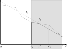
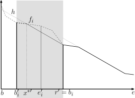
a)	b)

Figure 2: Iterative computation of $\mathrm{OptCost}_{\Gamma}(l^{*})$ over the interval $I=[b,e]$, where $l^{*}\in L^{\mathrm{Min}}$. Diagrams a) and b) depict two subsequent iterations; the gray rectangle indicates the subinterval for which the $\mathrm{OptCost}_{\Gamma}(l^{*})$ function is being computed during the given iteration.

Correctness and complexity.

We show that the procedure $\mathtt{SolveRP}$ is correct, i.e., that if it terminates, the output is in fact the $\mathrm{OptCost}$ function, and that it indeed terminates. We will also show, that there is an exponential upper bound on the running time of $\mathtt{SolveRP}$. The main result of this paper is as follows:

Theorem 15

Given a reachability-price game $\Gamma$, the function $\mathtt{SolveRP}(\Gamma)$ terminates and outputs the function $\mathrm{OptCost}_{\Gamma}$.

We will prove the Theorem in two steps. First, we prove that if the iterative procedure in cases 2 and 3 terminates, it computes $\mathrm{OptCost}$. Second, we show that it always terminates.

Theorem 16

Given a reachability-price game $\Gamma$, if $\mathtt{SolveRP}(\Gamma)$ terminates, it outputs the function $\mathrm{OptCost}_{\Gamma}$.

Proof 3.17.

The proof is inductive. Fix $\Gamma$, and let $l$ be the non-urgent location that minimizes $\pi(l)$. Assume that $\Gamma$ has $n+1$ non-urgent locations, and that Theorem 16 holds for every game $\Gamma^{\prime}$ that has at most $n$ non-urgent locations.

If there are no non-urgent locations, then computing $\mathrm{OptCost}_{\Gamma}$ amounts to solving a reachability-price game on a finite graph. It remains to prove the inductive step; there are two cases to consider. The first case, when $l\in L^{\mathrm{Min}}$ and the second case when $l\in L^{\mathrm{Max}}$. The proofs of these two cases follows from Lemmas 3.18 and 3.20.∎

Lemma 3.18.

Given a reachability-price game $\Gamma$ with the price-rate minimizing location in $L^{\mathrm{Max}}$, if Case 2 of $\mathtt{SolveRP}$ terminates, it outputs $\mathrm{OptCost}_{\Gamma}$.

Proof 3.19.

Case 2 is handled in the same way as in Bouyer’s et al. algorithm [10].∎

Lemma 3.20.

Given a reachability-price game $\Gamma$ with the price-rate minimizing location in $L^{\mathrm{Min}}$, if Case 3 of $\mathtt{SolveRP}$ terminates, it outputs $\mathrm{OptCost}_{\Gamma}$.

Proof 3.21.

Without loss of generality we assume that we are dealing with a single interval $I$. Let $l^{*}$, $\Gamma^{\prime}$, $\Gamma^{\prime\prime}$, $f$, and $x^{*}\in I$ be defined as in the Case 3 of the algorithm.

We will show that $\mathrm{OptCost}_{\Gamma^{\prime}}(l^{*})=\mathrm{OptCost}_{\Gamma}(l^{*})$ over the interval $[x^{*},e]$ and that $\mathrm{OptCost}_{\Gamma^{\prime\prime}}(l^{*})=\mathrm{OptCost}_{\Gamma}(l^{*})$ over the interval $[b,x^{*}]$. This, together with Lemmas 11 and 12 enables us to establish that the procedure for computing $\mathrm{OptCost}_{\Gamma}$ over $I$ in Case 3 is correct. By the inductive hypothesis, we can solve $\Gamma^{\prime}$ and $\Gamma^{\prime\prime}$ — these games have one less non-urgent location than $\Gamma$. Additionally, in games $\Gamma^{\prime}$ and $\Gamma^{\prime\prime}$ we restrict the minimizer so we immediately have:

$$\mathrm{OptCost}_{\Gamma^{{}^{\prime}/^{\prime\prime}}}(l)(x)\geqslant\mathrm{OptCost}_{\Gamma}(l)(x),$$

for every $l\in L$ and every $x\in[x^{*},e]/[b,x^{*}]$. By definition of $\Gamma^{\prime}$, there is an equality for $x=e$. To complete the proof, we need to show the reverse inequality.

There are two cases to consider. We start with the first case, i.e., we will show that $\mathrm{OptCost}_{\Gamma^{\prime}}(l^{*})\leqslant\mathrm{OptCost}_{\Gamma}(l^{*})$ over $[x^{*},e]$.

Fix $\varepsilon>0$ and a strategy $\mu\in\Sigma^{\mathrm{Min}}$ (note that $\Gamma$ and $\Gamma^{\prime}$ admit the same sets of strategies). We take $\chi_{\varepsilon}\in\Sigma^{\mathrm{Max}}$ that is $\varepsilon$-optimal for $\mu$ in $\Gamma^{\prime}$. For every $s\in\{l^{*}\}\times[x^{*},e]$ let $\omega$ denote the unique run $\mathrm{Run}(s,\mu,\chi_{\varepsilon})$, and lets assume it visits $l^{*}$ exactly $m$ times, after transitions $i_{1},\ldots,i_{m}$. We assume, without loss of generality, that after every such transition, a continuous one is taken. We then have:

$$\mathrm{Cost}_{\Gamma}(\omega) = \mathrm{Price}(\omega_{i_{m}})+\lambda_{i_{m}+1}\cdot\pi(l^{*})+\mathrm{Cost}_{\Gamma}(\mathrm{Run}(\omega_{i_{m}+1},\mu,\chi_{\varepsilon}))$$

$$\geqslant \mathrm{Price}(\omega_{i_{m}})+\lambda_{i_{m}+1}\cdot\pi(l^{*})+\mathrm{OptCost}_{\Gamma^{\prime}}(s_{i_{m}+1})-\varepsilon$$

$$\geqslant \mathrm{Price}(\omega_{i_{1}})+(x_{i_{m}}+\lambda_{i_{m}+1}-x_{i_{1}})\cdot\pi(l^{*})+\mathrm{OptCost}_{\Gamma}(s_{i_{m}+1})-\varepsilon$$

$$\geqslant \mathrm{Price}(\omega_{i_{1}})+(e-x_{i_{1}})\cdot\pi(l^{*})+\mathrm{OptCost}_{\Gamma}((l^{*},e))-\varepsilon$$

$$= \mathrm{OptCost}_{\Gamma^{\prime}}(s)-\varepsilon,$$

where $s_{i}=(l_{i},x_{i})$. The first inequality holds because $\chi_{\varepsilon}$ is $\varepsilon$-optimal for $\mu$ in $\Gamma^{\prime}$, and because the suffix of $\omega$ starting in $s_{i_{m}}$ does not visit $l^{*}$ but for the first transition, which comes at a price zero. The second inequality holds because $l^{*}$ minimizes $\pi(l^{*})$. The third inequality follows from the definition of $\mathrm{OptCost}_{\Gamma^{\prime}}(l^{*})$. Finally, $mathrm{Len}(\omega_{i_{1}})=0$, hence $\mathrm{Cost}(\omega_{i_{1}})=0$.

We now proceed to the second case, i.e., that $\mathrm{OptCost}_{\Gamma^{\prime\prime}}(l^{*})\leqslant\mathrm{OptCost}_{\Gamma}(l^{*})$ over $[b,x^{*}]$. The fact that $\mathrm{OptCost}_{\Gamma^{\prime\prime}}(l^{*})\leqslant\mathrm{OptCost}_{\Gamma^{\prime}}(l^{*})$ over $[b,x^{*}]$ implies that the slope of $f$ is shallower than $-\pi(l^{*})$.

Fix $\varepsilon>0$ and $\mu\in\Sigma^{\mathrm{Min}}$ in $\Gamma$. Let $\chi_{\varepsilon}\in\Sigma^{\mathrm{Max}}$ be a strategy that is $\varepsilon$-optimal for $\mu$ in $\Gamma^{\prime\prime}$ (the sets of strategies in $\Gamma$ and $\Gamma^{\prime\prime}$ are equal). For every $s\in\{l\}\times[b,x^{*}]$, let $\omega$ denote the unique run $\mathrm{Run}(s,\mu,\chi_{\varepsilon})$, which pays $m$ visits to $l^{*}$ (the notation and assumptions are the same as in the first case). We then have:

$$\mathrm{Cost}_{\Gamma}(\omega) = \mathrm{Price}(\omega_{i_{m}})+\lambda_{i_{m}+1}\cdot\pi(l^{*})+\mathrm{Cost}_{\Gamma}(\mathrm{Run}(\omega_{i_{m}+1},\mu,\chi_{\varepsilon^{\prime}}))$$

$$\geqslant \mathrm{Price}(\omega_{i_{m}})+\lambda_{i_{m}+1}\cdot\pi(l^{*})+\mathrm{OptCost}_{\Gamma^{\prime\prime}}(s_{i_{m}+1},\mu,\chi_{\varepsilon^{\prime}}))-\varepsilon$$

$$\geqslant \mathrm{Price}(\omega_{i_{1}})+(x_{i_{m}}+\lambda_{i_{m}+1}-x_{i_{1}})\cdot\pi(l^{*})+\mathrm{OptCost}_{\Gamma^{\prime\prime}}(s_{i_{m}+1})-\varepsilon$$

$$\geqslant \mathrm{Price}(\omega_{i_{1}})+\mathrm{OptCost}_{\Gamma^{\prime\prime}}(s_{i_{1}})-\varepsilon$$

$$= \mathrm{OptCost}_{\Gamma^{\prime\prime}}(s_{i_{1}})-\varepsilon.$$

The first inequality holds because $\omega$ does not feature transitions ending in $l^{*}$, modulo its prefix $\omega_{i_{m}+1}$, and because $\chi_{\varepsilon}$ is $\varepsilon$-optimal for $\mu$ in $\Gamma^{\prime\prime}$. The second inequality holds because $l^{*}$ minimizes $\pi(l^{*})$. The final inequality holds because the slope of $f$ is shallower than $-\pi(l^{*})$ over $[b,x^{*}]$. This finishes the proof of the theorem. ∎

We have proved that the algorithm is partially correct. It remains to prove its total correctness, i.e., that it terminates.

Theorem 3.22.

The algorithm $\mathtt{SolveRP}$ terminates.

Proof 3.23.

To prove termination of the algorithm, we need to prove the termination of the iterative procedures from cases 2 and 3 of the algorithm.

Each of the two cases is different, however, they have one thing in common. In each iteration, in both cases, an interval with slope shallower than $-\pi(l^{*})$ is processed. Since $l^{*}$ minimizes $\pi(l^{*})$, and by Lemmas 3 and 13, this interval corresponds to a segment of a goal cost function. We argue that the number of iterations in each case is bounded by the number of all the possible intersections of the cost functions assigned to goal locations, which is finite.

More precisely, let $\Gamma^{\prime}$, $I$, $f$ and $i$ be defined as in Case 2 of the algorithm. The slope of $f_{i}$ over $I_{i}$ is shallower than $-\pi(l^{*})$, so by Lemmas 3 and 13, $f_{i}$ coincides with some cost function over $I_{i}$ — denoted by $g$. If $i>1$, then there are two possibilities, either $b_{i}$ coincides with an intersection of cost functions from two different goal locations, or otherwise $f_{i-1}$ has the slope equal to $-\pi(l)$ for some non-goal location $l$.

In the first case, the iteration must have moved past one of the finitely many intersection points. In the second case, we need to argue that if the procedure once again encounters the same affine piece of $g$ (but over a different interval), then it must have also passed at least one of the finitely many intersection points. Let $I^{\prime}=[b^{\prime},e^{\prime}]\subseteq[b,b_{i})$ denote the interval over which the procedure encounters $g$ again. Assume that the procedure did not pass any intersection points before $I^{\prime}$. This implies that $\mathrm{OptCost}_{\Gamma^{\prime}}(l^{*})\geqslant g$ over $[e^{\prime},b_{i}]$, and hence $\mathrm{OptCost}_{\Gamma^{\prime}}(l^{*})$ must contain an affine piece that has a slope shallower than $g$ over $[e^{\prime},z]$, for some $z\in(e^{\prime},b_{i}]$. However, such a piece coincides with a goal cost function, so an intersection point must have been passed.

So far we have shown termination of the iterative procedure in Case 2. It remains to show the same for Case 3. Let $\Gamma^{\prime}$, $f$, $i$, and $x^{*}$ be defined as in Case 3 of the algorithm. We argue that each affine segment of a goal cost function is processed only once. If $i>1$, then $f_{i-1}$ either coincides with a different piece of a goal cost function, which means that we have passed one of the finitely many intersection points and the $f_{i}$ segment has been processed, or its slope is equal to $-\pi(l)$, for some non-goal location $l$. In the latter case, we have that $\mathrm{OptCost}_{\Gamma^{\prime}}(l^{*})$ has a slope steeper than $f_{i}$, and hence, it is strictly greater than $f_{i}$ over $[b,b_{i})$. This means that in the subsequent iterations, if $f_{i}$ is to be encountered, a piece with a slope smaller than that of $f_{i}$ needs to occur, but this means that an intersection point has been processed.

We have shown that in each step of the algorithm the iterative procedure of Cases 2 and 3 terminates, and hence, the algorithm terminates. ∎

We have proved that the procedure $\mathtt{SolveRP}$ is correct. The question that remains, is its complexity. We have the following result.

Theorem 3.24.

The algorithm $\mathtt{SolveRP}$ is in EXPTIME.

Proof 3.25.

Given an automaton $\mathcal{A}$, let $n$ denote the number of non-urgent locations and $p$ the total number of pieces in ${mathrm{CF}^{\mathrm{Goal}}}$. The complexity of computing the solution, using $\mathtt{SolveRP}$, depends on the number of pieces that constitute $\mathrm{OptCost}_{\Gamma}$. Let $N(n,p)$ denote the upper bound on the number of pieces in $\mathrm{OptCost}_{\Gamma}$. We now construct a recursion to characterise $N(n,p)$.

If $n=0$, then $N(n,p)=2p$ [10]. If $n>0$, both cases take $p$ (as argued in the proof of Theorem 3.22) iterations, and each requires solving two games with the solution complexity equal to $N(n-1,p+n)$ and $N(n-2,p+n-1)$. We can assume that $p>n$ is the case of real interest, so we have $N(n,p)\leqslant 2pN(n-1,2p)$. It can be easily verified that: $N(n,p)\leqslant 2^{\frac{(n+1)(n+2)}{2}}p^{n+1}$. This establishes that $\mathtt{SolveRP}$ is indeed in EXPTIME.∎

Discussion.

We now briefly compare our algorithm with that of Bouyer et al. The 3EXPTIME algorithm, introduced by Bouyer et al. [10], differs from the one presented in this paper in the way the minimizer locations are handled. As was explained above, the algorithm presented in this paper uses an iterative procedure, similar in spirit to that used for handling maximizer locations. The 3EXPTIME algorithm, on the other hand, exploited the following observation: if the location, $l$, which minimizes the weight function, is visited several times, then the minimizer would not be worse off, if, upon the first visit, she had waited the whole time that passes between the first and last visit — this is valid because all other locations have a higher value of the weight function. This intuition is formally captured by the algorithm in the following way. Two copies of the original automaton are created, with the only difference that in both of them $l$ becomes a goal location, and hence both automata have one less non-urgent location — this duplication introduces an exponential blowup in complexity. The first automaton captures the behavior before $l$ is entered for the first time, whereas the second copy captures the behaviour afterwords. In the second copy, $l$ is transformed into a goal location with a cost function equivalent to positive infinity — this captures the intuition, that it is sufficient to visit $l$ only once. The algorithm first computes $\mathrm{OptCost}$ for the second copy, then, using that result, computes $\mathrm{OptCost}$, for all states having $l$ as the location (this is in fact a game with a single non-urgent location), and finally computes $\mathrm{OptCost}$ for the first copy, with $\mathrm{OptCost}$, computed in the previous step, being assigned as a cost function to $l$. $\mathrm{OptCost}$ computed for the first copy is the sought solution. The second exponential blowup originated from the construction that allowed to assume that the clock value is bound by $1$. The construction used by Bouyer et al. [10] used locations to encode the integer part of the clock value, and the clock itself captured only the fractional part of the clock value — this yielded an exponential blowup, as there had to be a copy of the original location for every integer value between $0$ and the value of the largest constant provided in the definition of the automaton (recall, that constants are encoded in binary). Our construction, presented in Sec. 2, avoids this blowup.

References

- [1]
- [2] R. Alur & D. Dill (1994): A Theory of Timed Automata. Theoretical Computer Science 126(2), pp. 183–235. Available at http://portal.acm.org/citation.cfm?id=180519.
- [3] G. Behrmann, A. David & K. G. Larsen (2004): A Tutorial on UPPAAL. In: Formal Methods for the Design of Real-Time Systems. LNCS 3185, Springer, pp. 200–236. Available at http://www.springerlink.com/content/03wam998tjn5mgma/.
- [4] G. Behrmann, A. Fehnker, T. Hune, K. G. Larsen, P. Pettersson, J. Romijn & F. Vaandrager (2001): Minimum-Cost Reachability for Priced Timed Automata. In: HSCC’01. Lecture Notes in Computer Science 2034, Springer, pp. 147–161, 10.1007/3-540-45351-2. Available at http://portal.acm.org/citation.cfm?id=710599.
- [5] J. Berendsen, D. J. Jansen, J. Schmaltz & F. W. Vaandrager (2010): The axiomatization of override and update. Applied Logic 8(8), pp. 141–150, 10.1016/j.jal.2009.11.001. Available at http://www.sciencedirect.com/science/article/pii/S1570868309000676.
- [6] P. Bouyer, T. Brihaye, M. Jurdziński, R. Lazić & M. Rutkowski (2008): Average-Price and Reachability-Price Games on Hybrid Automata with Strong Resets. In: FORMATS’08. LNCS 5215, Springer, pp. 63–77, 10.1007/978-3-540-85778-5. Available at http://www.springerlink.com/content/a870592711j40661/.
- [7] P. Bouyer, T. Brihaye & N. Markey (2006): Improved Undecidability Results on Weighted Timed Automata. Information Processing Letters 98(5), pp. 188–194, 10.1016/j.ipl.2006.01.012. Available at http://portal.acm.org/citation.cfm?id=1711154.
- [8] P. Bouyer, E. Brinksma & K. G. Larsen (2004): Staying Alive as Cheaply as Possible. In: HSCC 2004. LNCS 2993, Springer, pp. 203–218. Available at http://www.lsv.ens-cachan.fr/~bouyer/mes-publis.php?onlykey=BBL-hscc2004.
- [9] P. Bouyer, E. Brinksma & K. G. Larsen (2008): Optimal Infinite Scheduling for Multi-Priced Timed Automata. Formal Methods in System Design 32(1), pp. 2–23, 10.1007/s10703-007-0043-4. Available at http://www.lsv.ens-cachan.fr/~bouyer/mes-publis.php?onlykey=BBL-fmsd06.
- [10] P. Bouyer, K. G. Larsen, N. Markey & J. I. Rasmussen (2006): Almost Optimal Strategies in One-Clock Priced Timed Automata. In: FSTTCS’06. LNCS 4337, Springer, pp. 345–356, 10.1007/11944836_32. Available at http://www.lsv.ens-cachan.fr/~markey/publis.php?onlykey=BLMR-fsttcs2006.
- [11] M. Jurdziński, R. Lazić & M. Rutkowski (2009): Average-Price-per-Reward Games on Hybrid Automata with Strong Resets. In: VMCAI’09. 5403, Springer, pp. 167 – 181, 10.1007/978-3-540-93900-9. Available at http://www.springerlink.com/content/57635657g2j60414/.
- [12] M. Jurdziński & A. Trivedi (2007): Reachability-Time Games on Timed Automata. In: ICALP’07. LNCS 4596, Springer, pp. 838–849, 10.1007/978-3-540-73420-8. Available at http://www.springerlink.com/content/b17738g23844w336/.
- [13] M. Jurdziński & A. Trivedi (2008): Average-Time Games. In: FSTTCS’08. LIPI 2, pp. 340–351, 10.4230/LIPIcs.FSTTCS.2008.1765. Available at http://drops.dagstuhl.de/opus/volltexte/2008/1765/.