QuantUM: Quantitative Safety Analysis of UML Models

Abstract

When developing a safety-critical system it is essential to obtain an assessment of different design alternatives. In particular, an early safety assessment of the architectural design of a system is desirable. In spite of the plethora of available formal quantitative analysis methods it is still difficult for software and system architects to integrate these techniques into their every day work. This is mainly due to the lack of methods that can be directly applied to architecture level models, for instance given as UML diagrams. Also, it is necessary that the description methods used do not require a profound knowledge of formal methods. Our approach bridges this gap and improves the integration of quantitative safety analysis methods into the development process. All inputs of the analysis are specified at the level of a UML model. This model is then automatically translated into the analysis model, and the results of the analysis are consequently represented on the level of the UML model. Thus the analysis model and the formal methods used during the analysis are hidden from the user. We illustrate the usefulness of our approach using an industrial strength case study.

1 Introduction

In a recent joint work with our industrial partner TRW Automotive GmbH we have proven the applicability of probabilistic verification techniques to safety analysis in an industrial setting [5]. The analysis approach that we used was that of probabilistic Failure Modes Effect Analysis (pFMEA) [13].

The most notable shortcoming of the approach that we observed lies in the missing connection of our analysis to existing high-level architecture models and the modeling languages that they are typically written in. TRW Automotive GmbH, like many other software development enterprises in the embedded systems domain, mostly uses the Unified Modeling Language (UML) [28] for system modeling. During the pFMEA we however had to use the language provided by the analysis tool that we used, in this case the input language of the stochastic model checker PRISM [15]. This required a manual translation from the design language UML to the formal modeling language PRISM. This manual translation has the following shortcomings: (1) It is a time-consuming and hence expensive process. (2) It is error-prone, since behaviors may be introduced that are not present in the original model. (3) The results of the formal analysis may not be easily transferable to the level of the high-level design language. To avoid problems that may result from (2) and (3), additional checks for plausibility have to be made, which again consume time. Some introduced errors may even remain unnoticed.

The objective of this paper is to bridge the gap between architectural design and formal stochastic modeling languages so as to remedy the negative implications of this gap listed above. This allows for a more seamless integration of formal dependability and reliability analysis into the design process. We propose an extension of the UML to capture probabilistic and error behavior information that are relevant for a formal stochastic analysis, such as when performing, for instance, pFMEA. All inputs of the analysis can be specified at the level of the UML model. In order to achieve this goal, we present an extension of the UML that allows for the annotation of UML models with quantitative information, such as for instance failure rates. Additionally, a translation process from UML models to the PRISM language is defined.

Structure of the paper.

The remainder of the paper is structured as follows: In Section 2 we present our QuantUM approach, in Section 3 we discuss the automatic construction of CSL formulas. The mapping of probabilistic counterexamples onto UML sequence diagrams is described in Section 4. Section 5 is devoted to the case study of an airbag system. Followed by a discussion of related work in Section 6. We conclude in Section 8.

2 The QuantUM Approach

In our approach all inputs of the analysis are specified at the level of a UML model. To facilitate the specification, we propose a quantitative extension of the UML. This extension is defined in terms of an UML Profile and takes advantage of the UML concept of a stereotype. Due to space restrictions, we can not elaborate all details of the proposed profile here, we will only present two central concepts, namely the QUMComponent stereotype and how the operational profile is captured with UML state machine diagrams. A comprehensive description of the profile can be found in [22].

The stereotype QUMComponent can be assigned to all UML elements that represent building blocks of the real system, which include classes, components and interfaces. Each element with the stereotype QUMComponent comprises up to one (hierarchical) state machine representing the normal behavior and between one and finitely many (hierarchical) state machines representing possible failure patterns. These state machines can be either state machines that are especially constructed for this QUMComponent, or they can be taken from a repository of state machines describing standard failure behaviors. The repository provides state machines for all standard components (e.g., switches) and the reuse of these state machines saves modeling effort and avoids redundant descriptions. In some cases, the normal behavior of a QUMComponent is not of interest for the analysis, for instance when describing failures of external components. In those cases the specification of the failure pattern state machines is sufficient. In addition, each QUMComponent comprises a list called Rates that contains rates together with names identifying them.

In order to capture the operational profile and particularly to allow the specification of quantitative information, such as failure rates, we extend the Transition element used in UML state machines with the stereotypes QUMAbstractStochasticTransition and QUMStochasticTransition. These stereotypes allow the user to specify transition rates as well as a name for the transition. The specified rates are used as transition rates for the continuous-time Markov chains that are generated for the purpose of stochastic analysis. Transitions with the stereotype QUMAbstractStochasticTransition are transitions that do not have a default rate. If a state machine is connected to a QUMComponent element, there has to be a rate in the Rates list of the QUMComponent that has the same name as the QUMAbstractStochasticTransition. This rate is then considered for the QUMAbstractStochasticTransition. The QUMAbstractStochasticTransition allows to define general state machines in a repository where the rates can be set individually for each component. The stereotypes QUMAbstractFailureTransition, QUMAbstractRepairTransition, QUMFailureTransition and QUMRepairTransition are specializations of QUMAbstractStochasticTransition and QUMStochasticTransition, respectively.

The normal behavior state machine and all failure pattern state machines of a QUMComponent are implicitly combined in one hierarchical state machine, cf. Figure 1. The combined state machine is automatically generated by the analysis tool and is not visible to the user. Its semantics can be described as follows: initially, the component executes the normal behavior state machine. If a QUMAbstractFailureTransition is enabled, the component will enter the state machine describing the corresponding failure pattern with the specified rate. The decision, which of the $n$ FailurePatterns is selected, is made by a stochastic ”race” between the transitions.

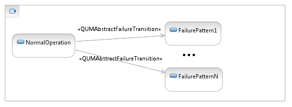
Figure 1: Combination of normal behavior and failure pattern state machines.

We define the semantics of QuantUM by defining a set of translation rules which map the UML artifacts that we defined to the input language of the model checker PRISM [15], which is considered to possess a formal semantics. This corresponds to the commonly held idea that the semantics of a UML model is largely defined by the underlying code generator. These translation rules enable a fully automated translation of the UML model into the PRISM language. We base our semantic transformation on the operational UML semantics defined in [21]. The counterexamples generated by our PRISM extension DiPro [6] are subsequently mapped onto fault trees and UML sequence diagrams, which makes them interpretable at the level of the UML model. Due to the fully automated nature of our approach the analysis model and the formal methods used during the analysis are completely hidden from the user.

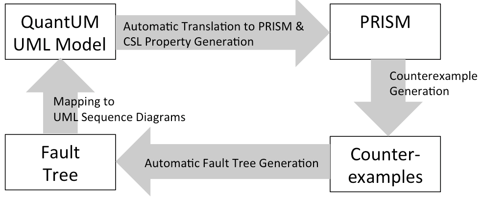
Figure 2: Overview of the QuantUM Approach.

Our approach depicted in Fig. 2 can be summarized by identifying the following steps:

• Our UML extension is used to annotate the UML model with all information that is needed to perform a dependability analysis.

• The annotated UML model is then exported in the XML Metadata Interchange (XMI) format [24] which is the standard format for exchanging UML models.

• Subsequently, our QuantUM Tool parses the generated XMI file and generates the analysis model in the input language of the probabilistic model checker PRISM as well the properties to be verified.

• For the analysis we use the probabilistic model checker PRISM together with DiPro in order to compute probabilistic counterexamples representing paths leading to a hazard state.

• The resulting counterexamples can then be transformed into a fault tree that can be interpreted at the level of the UML model. Alternatively, they can be mapped onto a UML sequence diagram which can be displayed in the UML modeling tool containing the original UML model.

In order to achieve the full automation that we argued for above it is important that a) the properties to be verified are automatically generated, and b) the counterexamples can be interpreted at the level of the UML model. We next discuss these two issues in more detail.

3 Automatic Generation of CSL Formulas

The properties to be analyzed are important inputs to the analysis of the QuantUM extended UML model. In stochastic model checking using PRISM, the property that is to be verified needs to be specified using a variant of temporal logic called Continuous Stochastic Logic (CSL) [2, 8]. We offer two possibilities for property specification: first we automatically generate a set of CSL properties out of the UML model, and second we allow the user to manually specify CSL properties.

We only give a brief introduction into CSL, for a more comprehensive description we refer to [8]. CSL is a stochastic variant of the Computation Tree Logic (CTL) [11] with state and path formulas based on [7]. The state formulas are interpreted over states of a continuous-time Markov chain (CTMC) [18], whereas the path formulas are interpreted over paths in a CTMC. CSL extends CTL with two probabilistic operators that refer to the steady state and transient behavior of the model. The steady-state operator refers to the probability of residing in a particular set of states, specified by a state formula, in the long run. The transient operator allows us to refer to the probability of the occurrence of particular paths in the CTMC. In order to express the time span of a certain path, the path operators until ($U$) and next ($X$) are extended with a parameter that specifies a time interval.

The automatic generation of CSL formulas out of the UML model requires the definition of a UML extension that allows us to refer to states of the UML model in the generated formulas. We introduce the stereotype QUMStateConfiguration (cf. Fig. 3) as part of our UML Profile described in [22]. This stereotype can be used to assign names to state configurations. In order to do so, the stereotype is assigned to states in the state machines of the UML model. All QUMStateConfiguration stereotypes with the same name are treated as one state configuration. This is reminiscent of labels in the PRISM language. A state configuration can also be seen as a boolean formula, each state can either be true when the system is in this state or false, when the system is not in this state. The operator variable indicates whether the boolean variables representing the states are connected by an and-operator (AND) or an or-operator (OR). The name of the state configuration is used during model to refer to these state configurations in the UML model.

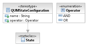
Figure 3: Definition of the QUMStateConfiguration stereotype.

We now discuss how the states of the UML model are translated into the PRISM model. For each QUMComponent, its states are encoded as integer values. States representing the normal behavior are always assigned a value between 0 and the total number of states representing normal behavior (#normstate). All failure states are identified by a number that is greater than #normstate. The placeholders %#normstate% and %#failstates% represent the number of states in the normal behavior state machine and failure pattern state machines respectively. The variable %module_id%_state is then used, in the PRISM model, to represent the states of the UML state machines, according to the state encoding explained above. Note that %module_id% will be replaced by an identifier which refers to the respective QUMComponent. The translation of the model to PRISM is done in linear time, by iterating over the QUMComponents.

In the following we describe how state formulas can automatically be generated by the QuantUM tool. The properties that we wish to generate fall into three categories:

• First we generate a property that can be used to compute the probability of a component to be in the failed state. This formula is generated for each component with the stereotype QUMComponent.

• Second, we generate a formula which computes the probability of the failure of any component, which means that at least one of the components with the stereotype QUMComponent is in a failure state.

• Third, we compute one formula for each QUMStateConfiguration that can be used to compute the probability of reaching this state configuration.

In the following we describe how formulas falling into these categories can be automatically generated.

Probability of the failure of a specified QUMComponent.

A QUMComponent is failed whenever it has entered a failure pattern state machine. Hence, whenever the value of the variable %module_id%_state is greater than %#normstate%, the component is failed. The resulting state formula representing the failure of a component is:

$$(\%\mbox{module\_id}\%\_\mbox{state}>\%\#\mbox{normstate}\%)$$

Thus, the CSL formula

$$P_{=?}[(\mbox{true})U^{<=T}(\%\mbox{module\_id}\%\_\mbox{state}>\%\#\mbox{normstate}\%)]$$

can be used to determine the probability of a failure of the QUMComponent with the specified module id within mission time T.

Probability of the failure of any QUMComponent.

The state formula

$$(\%\mbox{module\_id}_{1}\%\_\mbox{state}>\%\#\mbox{normstate}\%) |$$

$$(\%\mbox{module\_id}_{2}\%\_\mbox{state}>\%\#\mbox{normstate}\%) |...|$$

$$(\%\mbox{module\_id}_{n}\%\_\mbox{state}>\%\#\mbox{normstate}\%)$$

represents the failure of any of the components with module ids $\%\mbox{module\_id}_{1}\%...\%\mbox{module\_id}_{n}\%$. Similarly to the above, the CSL formula

$$P_{=?}[(\mbox{true})U^{<=T}((\%\mbox{module\_id}_{1}\%\_\mbox{state}>\%\#\mbox{normstate}\%) |$$

$$(\%\mbox{module\_id}_{2}\%\_\mbox{state}>\%\#\mbox{normstate}\%) |...|$$

$$(\%\mbox{module\_id}_{n}\%\_\mbox{state}>\%\#\mbox{normstate}\%))]$$

can be used to determine the probability of a failure of any of the QUMComponents within mission time T.

Probability of a QUMStateConfiguration.

As already explained, each QUMStateConfiguration can also be interpreted as a boolean formula. A state can then either be true, when the module is in this state or in one of its sub-states, or false, when the module is not in this state. The operator variable indicates whether the boolean variables representing the states are connected by a boolean and-operator (AND) or a boolean or-operator (OR). The states are identified by the state encoding explained above, hence the boolean expressions

$$\mbox{in\_state\_id}=(\mbox{state\_id}\leq\%\mbox{module\_id}\%\_\mbox{state}\leq\mbox{state\_id\_substate}_{n})$$

can be used to determine whether a QUMComponent is in a state with the state id in %state_id%, or in one of its sub-states. If the state with %state_id% does not have sub-states, the expression

$$\mbox{in\_state\_id}=(\%\mbox{module\_id}\%\_\mbox{state}=\%\mbox{state\_id}\%)$$

suffices. To obtain the complete state configuration we connect the individual formulas, identifying the single module states ($\mbox{in\_state\_id}_{1},...,\mbox{in\_state\_id}_{n}$ ) of the QUMStateConfiguration, by the appropriate Boolean operators. For the and-operator we get

$$\varphi=(\mbox{in\_state\_id}_{1}\&\mbox{in\_state\_id}_{2}\&...\&\mbox{in\_state\_id}_{n})$$

as state formula representing the QUMStateConfiguration, for the or-operator we get

$$\varphi=(\mbox{in\_state\_id}_{1}|\mbox{in\_state\_id}_{2}|...|\mbox{in\_state\_id}_{n})$$

respectively. In analogy to the previous cases, the CSL formula

$$P_{=?}[(\mbox{true})U^{<=T}(\varphi)]$$

can be used to determine the probability of reaching the QUMStateConfiguration within mission time T.

In addition to these three categories, we also generate the state formulas identifying the QUMStateConfiguration. These can be used to manually build more advanced CSL formulas in order to express more complicated properties. We propose to use the ProProST specification patterns [12] in order to obtain semantically correct CSL property specifications. It should be noted that according to the ProProST specification pattern system the CSL formulas that we generate all fall into the category of probabilistic existence. Also note that all formula patterns defined in [12] can be constructed with our tool using the state formulas that we synthesize.

4 Mapping of Probabilistic Counterexamples onto UML Sequence Diagrams

In order to hide the formal analysis model from the user, it is necessary to lift the results of the analysis to the level of the UML model. In a first step, we map the counterexamples generated by DiPro to Fault Trees [29]. This mapping is described in detail in [19] and is based on counterfactual-type causality reasoning [14]. For the purpose of this paper it suffices to say that we establish the causal relationships of the events of the model, that is transitions in the PRISM model, and the hazard (or other state formula) under consideration. This allows us to omit events from the counterexamples that are not causal for the hazard. The remaining events are then displayed in a fault tree. Even though the representation of the counterexamples as fault tree already lifts the counterexamples onto the level of the UML model and hence facilitates the analysis, it is still desirable to display the counterexamples in the same language as the model that is analyzed, namely UML. We therefore also describe a translation of the counterexample to UML Sequence Diagrams.

Since paths in a counterexample represent sequences of the system executions, UML sequence diagrams are an obvious choice to display probabilistic counterexamples. A sequence diagram in the UML is a type of interaction diagram, similar to Message Sequence Charts [16], that shows how processes interact with one another and in what order. An example of a UML sequence diagram can be found in Figure 4.

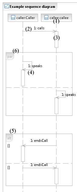
Figure 4: Example of a UML sequence diagram.

In a sequence diagram different processes or objects that live simultaneously are represented as parallel vertical lines, so called lifelines (cf. (1) in Figure 4). The messages exchanged between those objects are represented by horizontal arrows with the message name written above them (cf. (2) in Figure 4). Activation boxes, or method-call boxes, are opaque rectangles drawn on top of lifelines to represent that processes are being performed in response to the reception of a message (cf. (3) in Figure 4). Objects calling methods on themselves use messages and add new activation boxes on top of any other activation boxes to indicate a further level of processing (cf. (4) in Figure 4). The order of events along individual lifelines is total, from top to bottom. The order of potentially concurrent events across different lifelines is partial, in keeping with the happened-before relation of [20]. In order to impose a total order of events, message names can be labeled with natural numbers, as illustrated in Figure 10. Combined interaction fragments can be used to change this event order and to display alternative (alt) sequences (cf. (5) in Figure 4) or sequences that run concurrently (par) (cf. (6) in Figure 4).

Theoretically it is possible to map all paths of the counterexample directly to the sequence diagram. Since this mapping would result in a sequence diagram with hundreds of alternative sequences, it is necessary to extract those events from the counterexample that are causal for the hazard. This extraction is done by our fault tree computation algorithm. The paths of the counterexample returned by this algorithm are alternative execution paths of the system with the probability P. In order to express alternative executions in sequence diagrams, an alt combined interaction fragment is used. The probability of the path is given in the name of the corresponding alt combined interaction fragment. For each QUMComponent of the model we add a lifeline representing the component. We add a function transition(”source state”,”target state”) to each component, in order to visualize the transitions that are taken inside the component. A call to the transition function is added for each transition in the fault tree. If the transition is a call of an operation of a QUMComponent, an operation call from the caller component to the callee component is added to the sequence diagram. If the paths of the counterexample would be mapped directly to the sequence diagram, all paths, including possible interleavings of the paths, would be added to the sequence diagram. When the fault tree computation is used to filter the paths, it is checked whether the order of the events does have effect on the causality. If the order of the events does not have an effect on the causality, the events are represented by par combined fragments where each compartment represents one event. The compartments of the par combined fragment can be either executed in parallel or in any other possible concurrent interleaving. Otherwise, that is the order of the event is relevant, the events are mapped to a sequence representing their order.

In order to display the sequence diagrams, the QuantUM tool appends the XMI code of the diagram to the XMI file that contains the UML model. Thus, it can easily be imported in the UML CASE-tool that was used to edit the original UML design model.

5 Case Study

We have applied our modeling and analysis approach to a case study from the automotive embedded software domain. We performed an analysis of the design of an Electronic Control Unit for an Airbag system that is being developed at TRW Automotive GmbH, see also [5]. Note that the used probability values are merely approximate ”ballpark” numbers, since the actual values are intellectual property of our industrial partner TRW Automotive GmbH that we are not allowed to publish.

The airbag system architecture that we consider consists of two acceleration sensors whose task is to detect front or rear crashes, one microcontroller to perform the crash evaluation, and an actuator that controls the deployment of the airbag.

The deployment of the airbag is secured by two redundant protection mechanisms. The Field Effect Transistor (FET) controls the power supply for the airbag squibs. If the Field Effect Transistor is not armed, which means that the FET-Pin is not high, the airbag squib does not have enough electrical power to ignite the airbag. The second protection mechanism is the Firing Application Specific Integrated Circuit (FASIC) which controls the airbag squib. Only if it receives first an arm command and then a fire command from the microcontroller it will ignite the airbag squib.

Although airbags save lives in crash situations, they may be fatal if they are inadvertently deployed. This is because the driver may lose control of the car when this accidental deployment occurs. It is hence a pivotal safety requirement that an airbag is never deployed if there is no crash situation. In order to analyze how safe the considered system architecture, modeled with the CASE tool IBM Rational Software Architect and shown in Figure 5, is, we annotated the model with our QuantUM extension and performed an analysis with the QuantUM tool.

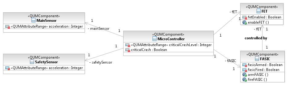
Figure 5: Class diagram modeling the airbag system.

The MicroController QUMComponent for instance, comprises one state machine representing its normal behavior (cf. Fig. 6) and one state machine representing the failure pattern, which is shown in Fig. 7. If the MicroController is in the normal state machine, it evaluates every 20ms whether there is a crash or not. If the MainSensor and the SafetySensor were giving readings above the threshold ($\mbox{ \em acceleration}>3$) for three consecutive evaluations, the MicroController concludes that there is a crash and the state $Crash$ is entered. In the Crash state, the FASIC is first armed, then the FET is enabled and finally, the FASIC is fired. The failure pattern of the MicroController can be entered at any time, with the rate specified for the QUMAbstractFailureTransition. As soon as it is entered it will execute the fire sequence: enable FET, arm FASIC, and fire FASIC.

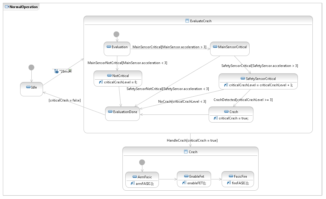
Figure 6: State machine representing the normal behavior of the microcontroller.

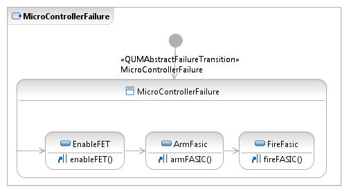
Figure 7: State machine representing the failure pattern of the microcontroller.

After all annotations were made, we exported the model into an XMI file, which was then imported by the QuantUM tool and translated into a PRISM model. The import of the XMI file and translation of the model was completed in less than two seconds. Without the QuantUM tool, this process would require days of work of a trained engineer.

The resulting PRISM model consists of 3249 states and 15390 transitions. The QuantUM tool also generated the CSL formula $P_{=?}[(\mbox{true})U^{<=T}(\mbox{\em inadvertent\_deployment})]$ where inadvertent_deployment is replaced by the state formula which identifies all states in the QUMStateConfiguration with the value inadvertent_deployment. T represents the mission time. Since the acceleration value of the sensor state machines is always zero, the formula $P_{=?}[(\mbox{true})U^{<=T}(\mbox{\em inadvertent\_deployment})]$ calculates the probability of the airbag being deployed, during the mission time $T$, when there is no crash situation. Owing to the use of the QuantUM tool, the only input which has to be given by the user is the mission time $T$.

We computed probabilities for the mission times T=10, T=100, and T=1000 and recorded the runtime for the counterexample computation (Runtime CX), the number of paths in the counterexample (Paths in CX), the runtime of the fault tree generation algorithm (Runtime FT) and the numbers of paths in the fault tree (Paths in FT) in Figure 8. The experiments where performed on a PC with an Intel QuadCore i5 processor with 2.67 Ghz and 8 GBs of RAM.

T	Runtime CX (sec.)	Paths in CX	Runtime FT (sec.)	Paths in FT
10	646.425 (approx. 10.77 min.)	738	2.86	5
100	664.893 (approx. 11.08 min.)	738	3.52	5
1000	820.431 (approx. 15.67 min.)	738	2.98	5

Figure 8: Experiment results for T=10, T=100 and T=1000.

Figure 8 shows that the computation of the fault tree is finished in several seconds, whereas the computation of the counterexample takes several minutes. While the different running times of the counterexample computation algorithm seem to be caused by the different values of the mission time $T$, the variation of the running time of the fault tree computation seems to be caused by background processes on the PC on which the experiments were conducted.

Figure 9 shows the fault tree generated from the counterexample for T=10. While the counterexample consists of 738 paths, the fault tree comprises only 5 paths. It is easy to see by which basic events, and with which probabilities, an inadvertent deployment of the airbag is caused. Obviously, there is only one single fault that can lead to an inadvertent deployment, namely FASICShortage. It is also easy to recognize that the basic event MicroControllerFailure, for instance, can only lead to an inadvertent deployment if it is followed by one of the following sequences of basic events: enableFET, armFASIC, and fireFASIC or enableFET, and FASICStuckHigh. If the basic event FETStuckHigh occurs prior to the MicroControllerFailure, then the sequence armFASIC and fireFASIC occurring after the MicroControllerFailure event suffices.

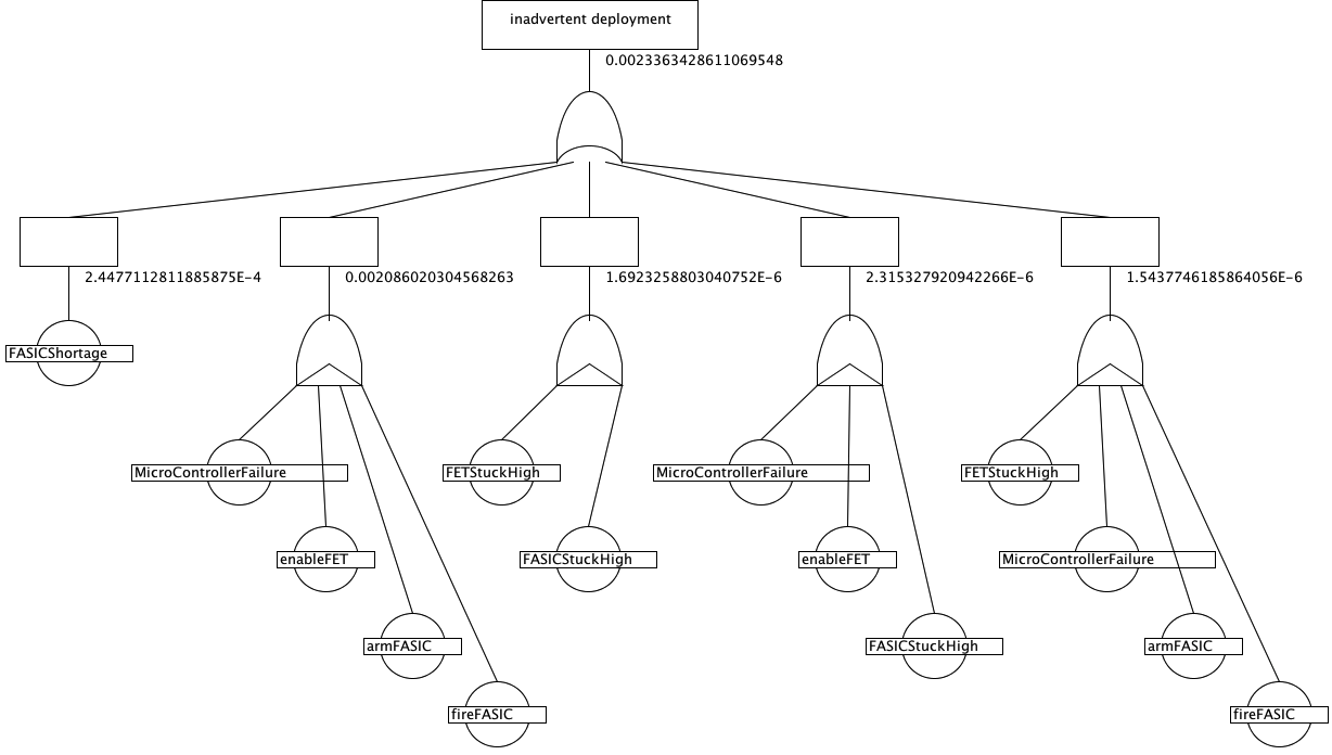
Figure 9: Fault tree for the QUMStateConfiguration inadvertent_deployment (T = 10).

The case study shows that the fault tree is a compact and concise visualization of the counterexample which allows for an easy identification of the basic events that cause the inadvertent deployment of the airbag, and their corresponding probabilities. If the order of the events is important, this can be seen in the fault tree by the PAND-gate. Using a manual analysis one would have to manually compare the order of the events in all 738 paths in the counterexample, which is a tedious and time consuming task.

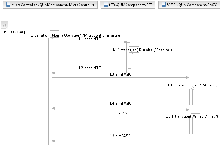
Figure 10: Fragment of the UML sequence diagram for the QUMStateConfiguration inadvertent_deployment (T = 10).

Figure 10 shows a fragment of the UML sequence diagram which visualizes the counterexample for T=10. The generation of the XMI code of the sequence diagram took less then one second. We imported the XMI code into the UML model of the airbag system in the CASE tool IBM Rational Software Architect. This allows us to interpret the counterexample directly in the CASE tool. An additional benefit of the visualization of the counterexample as a sequence diagram is that operation calls can be depicted. In Figure 10, for instance, it is easy to see how after a failure of the microcontroller the operations enableFET(), armFASIC(), and fireFASIC() are called.

6 Related Work

The idea of using UML models to derive models for quantitative safety analysis is not new. In [23] the authors present a UML profile for annotating software dependability properties. This annotated model is then transformed into an intermediate model, that is then transformed into Timed Petri Nets. The main drawbacks of this work is that it merely focuses on the structural aspect of the UML model, while the actual behavioral description is not considered. Another drawback is the introduction of unnecessary redundant information in the UML model, since sometimes the joint use of more than one stereotype is required. In [9] the authors extend the UML Profile for Modeling and Analysis of Real Time Embedded Systems (MARTE) [25] with a profile for dependability analysis and modeling. While this work is very expressive, it heavily relies on the use of the MARTE profile, which is only supported by very few UML CASE tools. Additionally, the amount of stereotypes, tagged values and annotations that need to be added to the model is very large. Another drawback of this approach is that the translation from the annotated UML model into the Deterministic and Stochastic Petri Nets (DSPN) [3] used for analysis is carried out manually which is, as we argue above, an error-prone and risky task for large UML models. The work defined in [17] presents a stochastic extension of the Statechart notation, called StoCharts. The StoChart approach suffers from the following drawbacks. First, it is restricted to the analysis of the behavioral aspects of the system and does not allow for structural analysis. Second, while there exist some tools that allow to draw StoCharts, there is no integration of StoCharts into UML models available. In [10] the architecture dependability analysis framework Arcades is presented. While Arcade is very expressive and was applied to hardware, software and infrastructure systems, the main drawback is that it is based on a textual description of the system and hence would require a manual translation process of the UML model to Arcade.

We are, to the best of our knowledge, not aware of any alternative approach that allows for the automatic generation of the analysis model and the automatic CSL property construction.

7 Future Work

In future work we plan to extend the expressiveness of the QuantUM profile, to integrate methods to further facilitate automatic stochastic property specification, and to apply our approach on other architecture description languages such as, for instance, SysML [27].

At the moment the approach can be applied to all system and software architecture models that do not make use of complex programming code in the entry-, during- or exit-action of the states. To further extend our approach we plan to work on methods for the probabilistic analysis of object-oriented source code attached to state machine transitions.

Additionally, we plan to conduct more case studies to prove the scalability of our approach.

8 Conclusion

We have presented an UML profile that allows for the annotation of UML models with quantitative information, together with a tool that automatically translates the model into the PRISM language and performs the analysis with PRISM. In addition to the translation of the model, the tool also allows for the automatic generation of CSL properties. Furthermore, we have developed a method, not described in detail in this paper, that automatically generates a fault tree from a probabilistic counterexample. The resulting fault trees were significantly smaller than the probabilistic counterexamples and hence easier to understand, while still presenting all causally relevant information. We also presented a mapping of probabilistic counterexamples to UML sequence diagrams which make the counterexamples interpretable inside the UML modeling tool. We believe that this is particularly useful for system and software architects which usually can interpret an UML sequence diagram much better than fault trees, whereas safety engineers might prefer the visualization of the counterexamples as fault trees. We illustrated the usefulness of our modeling and analysis approach using an industrial case study.

References

- [1]
- [2] A. Aziz, K. Sanwal, V. Singhal & R. K. Brayton (1996): Verifying Continuous-Time Markov Chains. In: CAV ’96: Proceedings of the 8th International Conference on Computer Aided Verification, 1102, Springer Verlag LNCS, New Brunswick, NJ, USA, pp. 269–276, 10.1007/3-540-61474-5_75.
- [3] M. Ajmone Marsan & G. Chiola (1987): On Petri nets with deterministic and exponentially distributed firing times. Advances in Petri Nets 1987, pp. 132–145, 10.1007/3-540-18086-9_23.
- [4] H. Aljazzar & S. Leue (2008): Debugging of Dependability Models Using Interactive Visualization of Counterexamples. In: QEST ’08: Proceedings of the Fifth International Conference on the Quantitative Evaluation of Systems, IEEE Computer Science Press, pp. 189–198, 10.1109/QEST.2008.40.
- [5] Husain Aljazzar, Manuel Fischer, Lars Grunske, Matthias Kuntz, Florian Leitner-Fischer & Stefan Leue (2009): Safety Analysis of an Airbag System Using Probabilistic FMEA and Probabilistic Counterexamples. In: QEST ’09: Proceedings of the Sixth International Conference on Quantitative Evaluation of Systems, IEEE Computer Society, Los Alamitos, CA, USA, pp. 299–308, 10.1109/QEST.2009.8.
- [6] Husain Aljazzar & Stefan Leue (2009): Directed Explicit State-Space Search in the Generation of Counterexamples for Stochastic Model Checking. IEEE Transactions on Software Engineering, 36(1), pp. 37–60, 10.1109/TSE.2009.57.
- [7] Adnan Aziz, Kumud Sanwal, Vigyan Singhal & Robert Brayton (2000): Model-Checking Continuous-Time Markov Chains. ACM Trans. Comput. Logic 1(1), pp. 162–170, 10.1145/343369.343402.
- [8] Christel Baier, Boudewijn Haverkort, Holger Hermanns & Joost-Pieter Katoen (2003): Model-Checking Algorithms for Continuous-Time Markov Chains. IEEE Transactions on Software Engineering 29(7), pp. 524–541, 10.1109/TSE.2003.1205180.
- [9] S. Bernardi, J. Merseguer & D.C. Petriu (2009): A dependability profile within MARTE. Software and Systems Modeling , pp. 1–24, 10.1007/s10270-009-0128-1.
- [10] H. Boudali, P. Crouzen, B.R. Haverkort, M. Kuntz & M.I.A. Stoelinga (2008): Architectural Dependability Modelling with Arcade. In: Proceedings of the 38th Annual IEEE/IFIP International Conference on Dependable Systems and Networks, pp. 512–521, 10.1109/DSN.2008.4630122.
- [11] E. M. Clarke, E. A. Emerson & A. P. Sistla (1986): Automatic verification of finite-state concurrent systems using temporal logic specifications. ACM Transactions on Programming Languages and Systems 8(2), pp. 244–263, 10.1145/5397.5399.
- [12] Lars Grunske (2008): Specification patterns for probabilistic quality properties. In: ICSE ’08: Proceedings of the 30th international conference on Software engineering, ACM, New York, NY, USA, pp. 31–40, 10.1145/1368088.1368094.
- [13] Lars Grunske, Robert Colvin & Kirsten Winter (2007): Probabilistic Model-Checking Support for FMEA. In: QEST ’07: Proceedings of the Fourth International Conference on Quantitative Evaluation of Systems, IEEE Computer Society, Washington, DC, USA, pp. 119–128, 10.1109/QEST.2007.34.
- [14] J.Y. Halpern & J. Pearl (2005): Causes and explanations: A structural-model approach. Part I: Causes. The British journal for the philosophy of science 56(4), p. 843-–887, 10.1093/bjps/axi147.
- [15] A. Hinton, M. Kwiatkowska, G. Norman & D. Parker (2006): PRISM: A Tool for Automatic Verification of Probabilistic Systems. In: TACAS ’06: Proceedings of the 12th International Conference on Tools and Algorithms for the Construction and Analysis of Systems, Lecture Notes in Computer Science, Springer, pp. 441–444, 10.1007/11691372_29.
- [16] ITU-TS recommendation Z.120 (1996): Message Sequence Chart (MSC).
- [17] David Nicolaas Jansen (2003): Extensions of statecharts : with probability, time, and stochastic timing. Ph.D. thesis, University of Twente. Available at http://doc.utwente.nl/58230/.
- [18] V.G. Kulkarni (1995): Modeling and analysis of stochastic systems. Chapman & Hall/CRC.
- [19] Matthias Kuntz, Florian Leitner-Fischer & Stefan Leue (2011): From Probabilistic Counterexamples via Causality to Fault Trees. Technical Report soft-11-02, Chair for Software Engineering, University of Konstanz. Available at http://www.inf.uni-konstanz.de/soft/research/publications/pdf/soft-11-02.pdf.
- [20] Leslie Lamport (1978): Time, clocks, and the ordering of events in a distributed system. Commun. ACM 21, pp. 558–565, 10.1145/359545.359563.
- [21] D. Latella, I. Majzik, M. Massink et al. (1999): Towards a formal operational semantics of UML statechart diagrams. In: IFIP TC6/WG6, 1, Citeseer, pp. 331–347.
- [22] Florian Leitner-Fischer (2010): Quantitative Safety Analysis of UML Models. Master’s thesis, University of Konstanz. Available at http://kops.ub.uni-konstanz.de/volltexte/2010/12520/.
- [23] I. Majzik, A. Pataricza & A. Bondavalli (2003): Stochastic dependability analysis of system architecture based on UML models. Architecting dependable systems , pp. 219–244, 10.1007/3-540-45177-3_10.
- [24] Object Management Group (2007): XML Metadata Interchange (XMI), v2.1.1. http://www.omg.org/technology/documents/formal/xmi.htm.
- [25] Object Management Group (2008): UML Profile for Modeling and Analysis of Real Time Embedded Systems. http://www.omgmarte.org/.
- [26] Object Management Group (2010): Object Constraint Language (OCL), v2.2. http://www.omg.org/spec/OCL/2.2/.
- [27] Object Management Group (2010): SysML. Specification v1.2. http://www.sysml.org.
- [28] Object Management Group (2010): Unified Modeling Language. Specification v2.3. http://www.uml.org.
- [29] U.S. Nuclear Regulatory Commission (1981): Fault Tree Handbook. NUREG-0492.