Integrating Generic Sensor Fusion Algorithms with Sound State Representations through Encapsulation of Manifolds

Abstract

Common estimation algorithms, such as least squares estimation or the Kalman filter, operate on a state in a state space $\mathcal{S}$ that is represented as a real-valued vector. However, for many quantities, most notably orientations in 3D, $\mathcal{S}$ is not a vector space, but a so-called manifold, i.e. it behaves like a vector space locally but has a more complex global topological structure. For integrating these quantities, several ad-hoc approaches have been proposed.

Here, we present a principled solution to this problem where the structure of the manifold $\mathcal{S}$ is encapsulated by two operators, state displacement $\mathbin{\text{\raisebox{-0.86108pt}{$\boxplus$}}}:\mathcal{S}\times\mathbb{R}^{n}\to\mathcal{S}$ and its inverse $\mathbin{\text{\raisebox{-0.86108pt}{$\boxminus$}}}:\mathcal{S}\times{}\mathcal{S}\to\mathbb{R}^{n}$. These operators provide a local vector-space view $\delta\mapsto{}x\mathbin{\text{\raisebox{-0.86108pt}{$\boxplus$}}}\delta$ around a given state $x$. Generic estimation algorithms can then work on the manifold $\mathcal{S}$ mainly by replacing $+/-$ with $\mathbin{\text{\raisebox{-0.86108pt}{$\boxplus$}}}$/$\mathbin{\text{\raisebox{-0.86108pt}{$\boxminus$}}}$ where appropriate. We analyze these operators axiomatically, and demonstrate their use in least-squares estimation and the Unscented Kalman Filter. Moreover, we exploit the idea of encapsulation from a software engineering perspective in the Manifold Toolkit, where the $\mathbin{\text{\raisebox{-0.86108pt}{$\boxplus$}}}$/$\mathbin{\text{\raisebox{-0.86108pt}{$\boxminus$}}}$ operators mediate between a “flat-vector” view for the generic algorithm and a “named-members” view for the problem specific functions.

red

1 Introduction

Sensor fusion is the process of combining information obtained from a variety of different sensors into a joint belief over the system state. In the design of a sensor fusion system, a key engineering task lies in finding a state representation that (a) adequately describes the relevant aspects of reality and is (b) compatible with the sensor fusion algorithm in the sense that the latter yields meaningful or even optimal results when operating on the state representation.

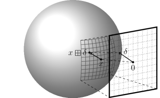
Figure 1: Mapping a local neighborhood in the state space (here: on the unit sphere $S^{2}$) into $\mathbb{R}^{n}$ (here: the plane) allows for the use of standard sensor fusion algorithms without explicitly encoding the global topological structure.

Satisfying both these goals at the same time has been a long-standing challenge. Standard sensor fusion algorithms typically operate on real valued vector state representations ($\mathbb{R}^{n}$) while mathematically sound representations often form more complex, non-Euclidean topological spaces. A very common example of this comes up, e.g. within the context of inertial navigation systems (INS) where a part of the state space is $SO(3)$, the group of orientations in $\mathbb{R}^{3}$. To estimate variables in $SO(3)$, there are generally two different approaches. The first uses a parameterization of minimal dimension, i.e. with three parameters (e.g. Euler angles), and operates on the parameters like on $\mathbb{R}^{3}$. This parameterization has singularities, i.e. a situation analogous to the well-known gimbal lock problem in gimbaled INS [13] can occur where very large changes in the parameterization are required to represent small changes in the state space. Workarounds for this exist that try to avoid these parts of the state space, as was most prominently done in the guidance system of the Apollo Lunar Module [22], or switch between alternative orderings of the parameterization each of which exhibit singularities in different areas of the state space. The second alternative is to overparameterize states with a non-minimal representation such as unit quaternions or rotation matrices which are treated as $\mathbb{R}^{4}$ or $\mathbb{R}^{3\times 3}$ respectively and re-normalized as needed [45, 30]. This has other disadvantages such as redundant parameters or degenerated, non-normalized variables.

Both approaches require representation-specific modifications of the sensor fusion algorithm and tightly couple the state representation and the sensor fusion algorithm, which is then no longer a generic black box but needs to be adjusted for every new state representation.

Our approach is based on the observation that sensor fusion algorithms employ operations which are inherently local, i.e. they compare and modify state variables in a local neighborhood around some reference. We thus arrive at a generic solution that bridges the gap between the two goals above by viewing the state space as a manifold. Informally speaking, every point of a manifold has a neighborhood that can be mapped bi-directionally to $\mathbb{R}^{n}$. This enables us to use an arbitrary manifold $\mathcal{S}$ as the state representation while the sensor fusion algorithm only sees a locally mapped part of $\mathcal{S}$ in $\mathbb{R}^{n}$ at any point in time. For the unit sphere $S^{2}$ this is illustrated in figure 1.

We propose to implement the mapping by means of two encapsulation operators $\mathbin{\text{\raisebox{-0.86108pt}{$\boxplus$}}}$ (“boxplus”) and $\mathbin{\text{\raisebox{-0.86108pt}{$\boxminus$}}}$ (“boxminus”) where

$$\mathbin{\text{\raisebox{-0.86108pt}{$\boxplus$}}} :\mathcal{S}\times\mathbb{R}^{n} \to\mathcal{S},$$ (1)

$$\mathbin{\text{\raisebox{-0.86108pt}{$\boxminus$}}} :\mathcal{S}\times\mathcal{S} \to\mathbb{R}^{n}.$$ (2)

Here, $\mathbin{\text{\raisebox{-0.86108pt}{$\boxplus$}}}$ takes a manifold state and a small change expressed in the mapped local neighborhood in $\mathbb{R}^{n}$ and applies this change to the state to yield a new, modified state. Conversely, $\mathbin{\text{\raisebox{-0.86108pt}{$\boxminus$}}}$ determines the mapped difference between two states.

The encapsulation operators capture an important duality: The generic sensor fusion algorithm uses $\mathbin{\text{\raisebox{-0.86108pt}{$\boxminus$}}}$ and $\mathbin{\text{\raisebox{-0.86108pt}{$\boxplus$}}}$ in place of the corresponding vector operations $-$ and $+$ to compare and to modify states, respectively – based on flattened perturbation vectors – and otherwise treats the state space as a black box. Problem-specific code such as measurement models, on the other hand, can work inside the black box, and use the most natural representation for the state space at hand. The operators $\mathbin{\text{\raisebox{-0.86108pt}{$\boxplus$}}}$ and $\mathbin{\text{\raisebox{-0.86108pt}{$\boxminus$}}}$ translate between these alternative views. We will later show how this can be modeled in an implementation framework such that manifold representations (with matching operators) even of very sophisticated compound states can be generated automatically from a set of manifold primitives (in our C++ implementation currently $\mathbb{R}^{n}$, $SO(2)$, $SO(3)$, and $S^{2}$).

This paper extends course material [11] and several master’s theses [25, 5, 16, 43]. It starts with a discussion of related work in Section 2. Section 3 then introduces the $\mathbin{\text{\raisebox{-0.86108pt}{$\boxplus$}}}$-method and 3D orientations as the most important application, and Section 4 lays out how least squares optimization and Kalman filtering can be modified to operate on these so-called $\mathbin{\text{\raisebox{-0.86108pt}{$\boxplus$}}}$-manifolds. Section 5 introduces the aforementioned software toolkit, and Section 6 shows practical experiments. Finally, the appendices prove the properties of $\mathbin{\text{\raisebox{-0.86108pt}{$\boxplus$}}}$-manifolds claimed in Section 3 and give $\mathbin{\text{\raisebox{-0.86108pt}{$\boxplus$}}}$-manifold representations of the most relevant manifolds $\mathbb{R}/2\pi\mathbb{Z}$, $SO(n)$, $S^{n}$ and $\mathbb{P}^{n}$ along with proofs.

2 Related Work

2.1 Ad-hoc Solutions

Several ad-hoc methods are available to integrate manifolds into estimation algorithms working on $\mathbb{R}^{n}$ [37, 42]. All of them have some drawbacks, as we now discuss using 3D orientations as a running example.

The most common workaround is to use a minimal parameterization (e.g. Euler angles) [37] [42, p. 6] and place the singularities in some part of the workspace that is not used (e.g. facing $90^{\circ}$ upwards). This, however, creates an unnecessary constraint between the application and the representation leading to a failure mode that is easily forgotten. If it is detected, it requires a recovery strategy, in the worst case manual intervention as in the aforementioned Apollo mission [22].

Alternatively, one can switch between several minimal parameterizations with different singularities. This works but is more complicated.

For overparameterizations (e.g. quaternions), a normalization constraint must be maintained (unit length), e.g. by normalizing after each step [45, 30]. The step itself does not know about the constraint, and tries to improve the fit by violating the constraint, which is then undone by normalization. This kind of counteracting updates is inelegant and at least slows down convergence. Lagrange multipliers could be used to enforce the constraint exactly [42, p.40] but lead to a more difficult equation system. Alternatively, one could add the normalization constraint as a “measurement” but this is only an approximation, since it would need to have uncertainty zero [42, p.40].

Instead, one could allow non-normalized states and apply a normalization function every time before using them [27, 42]. Then the normalization degree of freedom is redundant having no effect on the cost function and the algorithm does not try to change it. Some algorithms can handle this (e.g. Levenberg-Marquardt [35, Chap. 15]) but many (e.g. Gauss-Newton [35, Chap. 15]) fail due to singular equations. This problem can be solved by adding the normalization constraint as a “measurement” with some arbitrary uncertainty. [42, p.40]. Still, the estimated state has more dimensions than necessary and computation time is increased.

2.2 Reference State with Perturbations

Yet another way is to set a reference state and work relative to it with a minimal parameterization [37, 42, p.6]. Whenever the parameterization becomes too large, the reference system is changed accordingly [1, 7]. This is practically similar to the $\mathbin{\text{\raisebox{-0.86108pt}{$\boxplus$}}}$-method, where in $s\mathbin{\text{\raisebox{-0.86108pt}{$\boxplus$}}}\delta$ the reference state is $s$ and $\delta$ is the minimal parameterization. In particular [7] has triggered our investigation, so we compare to their SPmap in detail in App. D. The vague idea of applying perturbations in a way more specific than by simply adding has been around in the literature for some time:

“We write this operation [the state update] as $x\rightarrow{}x+\delta{}x$, even though it may involve considerable more than vector addition.”       W. Triggs [42, p. 7]

Very recently, Strasdat et al. [39, Sec. II.C] have summarized this technique for $SO(3)$ under the label Lie group/algebra representation. This means the state is viewed as an element of the Lie group $SO(3)$, i.e. an orthonormal matrix or quaternion but every step of the estimation algorithm operates in the Lie group’s tangential space, i.e. the Lie algebra. The Lie’s group’s exponential maps a perturbation $\delta$ from the Lie algebra to the Lie group. For Lie groups this is equivalent to our approach, with $s\mathbin{\text{\raisebox{-0.86108pt}{$\boxplus$}}}\delta=s\cdot\exp\delta$ (Sec. A.6).

Our contribution here compared to [7, 42, 39] is to embed this idea into a mathematical and algorithmic framework by means of an explicit axiomatization, where the operators $\mathbin{\text{\raisebox{-0.86108pt}{$\boxplus$}}}$ and $\mathbin{\text{\raisebox{-0.86108pt}{$\boxminus$}}}$ make it easy to adapt algorithms operating on $\mathbb{R}^{n}$. Moreover, our framework is more generic, being applicable also to manifolds which fail to be Lie groups, such as $S^{2}$.

In summary, the discussion shows the need for a principled solution that avoids singularities and needs neither normalization constraints nor redundant degrees of freedom in the estimation algorithm.

2.3 Quaternion-Based Unscented Kalman Filter

A reasonable ad-hoc approach for handling quaternions in an EKF/UKF is to normalize, updating the covariance with the Jacobian of the normalization as in the EKF’s dynamic step [8]. This is problematic, because it makes the covariance singular. Still the EKF operates as the innovation covariance remains positive definite. Nevertheless, it is unknown if this phenomen causes problems, e.g. the zero-uncertainty degree of freedom could create overconfidence in another degree of freedom after a non-linear update.

With a similar motivation, van der Merwe [33] included a dynamic, $\dot{q}=\eta(1-|q|^{2})q$ that drives the quaternion $q$ towards normalization. In this case the measurement update can still violate normalization, but the violation decays over time.

Kraft [24] and Sipos [38] propose a method of handling quaternions in the state space of an Unscented Kalman Filter (UKF). Basically, they modify the unscented transform to work with their specific quaternion state representation using a special operation for adding a perturbation to a quaternion and for taking the difference of two quaternions.

Our approach is related to Kraft’s work in so far as we perform the same computations for states containing quaternions. It is more general in that we work in a mathematical framework where the special operations are encapsulated in the $\mathbin{\text{\raisebox{-0.86108pt}{$\boxplus$}}}$/$\mathbin{\text{\raisebox{-0.86108pt}{$\boxminus$}}}$-operators. This allows us to handle not just quaternions, but general manifolds as representations of both states and measurements, and to routinely adapt estimation algorithms to manifolds without sacrificing their genericity.

2.4 Distributions on Unit Spheres

The above-mentioned methods as well as the present work treat manifolds locally as $\mathbb{R}^{n}$ and take care to accumulate small steps in a way that respects the global manifold structure. This is an approximation as most distributions, e.g. Gaussians, are strictly speaking not local but extend to infinity. In view of this problem, several generalizations of normal distributions have been proposed that are genuinely defined on a unit sphere.

The von Mises-Fisher distribution on $S^{n-1}$ was proposed by Fisher [10] and is given by

$$\operatorname{\operatorname{p}}(x)=C_{n}(\kappa)\exp\!\left(\kappa\mu^{\top}x\right),$$ (3)

with $\mu,x\in S^{n-1}\subset\mathbb{R}^{n}$, $\kappa>0$ and a normalization constant $C_{n}(\kappa)$. $\mu$ is called the mean direction and $\kappa$ the concentration parameter.

For the unit-circle $S^{1}$ this reduces to the von Mises distribution

$$\operatorname{\operatorname{p}}(x)=C_{2}(\kappa)\exp\!\left(\kappa\cos(x-\mu)\right),$$ (4)

with $x,\mu\in[-\pi,\pi)$.

The von Mises-Fisher distribution locally looks like a normal distribution $\operatorname{\mathcal{N}}\!\left(0,\,\frac{1}{\kappa}\operatorname{I}_{n-1}\right)$ (viewed in the tangential space), where $\operatorname{I}_{n-1}$ is the $(n-1)$-dimensional unit matrix. As only a single parameter exists to model the covariance, only isotropic distributions can be modeled, i.e. contours of constant probability are always circular. Especially for posterior distributions arising in sensor fusion this is usually not the case.

To solve this, i.e. to represent general multivariate normal distributions, Kent proposed the Fisher-Bingham distribution on the sphere [21]. It is defined as:

$$\operatorname{\operatorname{p}}(x)=\tfrac{1}{c(\kappa,\beta)}\exp\!\left(\kappa\gamma_{1}^{\top}x+\beta[(\gamma_{2}^{\top}x)^{2}-(\gamma_{3}^{\top}x)^{2}]\right).$$

It requires $\gamma_{i}$ to be a system of orthogonal unit vectors, with $\gamma_{1}$ denoting the mean direction (as $\mu$ in the von Mises-Fisher case), $\gamma_{2}$ and $\gamma_{3}$ describing the semi-major and semi-minor axis of the covariance. $\kappa$ and $\beta$ describe the concentration and eccentricity of the covariance.

Though being mathematically more profound, these distributions have the big disadvantage that they can not be easily combined with other normal distributions. Presumably, a completely new estimation algorithm would be needed to compensate for this, whereas our approach allows us to adapt established algorithms.

3 The $\mathbin{\text{\raisebox{-0.86108pt}{$\boxplus$}}}$-Method

In this paper, we propose a method, the $\mathbin{\text{\raisebox{-0.86108pt}{$\boxplus$}}}$-method, which integrates generic sensor fusion algorithms with sophisticated state representations by encapsulating the state representation structure in an operator $\mathbin{\text{\raisebox{-0.86108pt}{$\boxplus$}}}$.

In the context of sensor fusion, a state refers to those aspects of reality that are to be estimated. The state comprises the quantities needed as output for a specific application, such as the guidance of an aircraft. Often, additional quantities are needed in the state in order to model the behavior of the system by mathematical equations, e.g. velocity as the change in position.

Figure 2: From reality to state representation in the INS example (see text for details). Step 1 models relevant aspects of reality in the state model. Step 2a uses the standard approach to obtain a lossy state representation. Step 2b uses the $\mathbin{\text{\raisebox{-0.86108pt}{$\boxplus$}}}$-method to obtain a state representation preserving the topological structure of the state space (using a faithful representation $SO(3)^{*}$ of $SO(3)$).

The first step in the design of a sensor fusion system (cf. Figure 2) is to come up with a state model based on abstract mathematical concepts such as position or orientation in three-dimensional space. In the aircraft example, the INS state would consist of three components: the position ($\mathbb{R}^{3}$), orientation ($SO(3)$), and velocity ($\mathbb{R}^{3}$), each in some Earth-centric coordinate system, i.e.

$$\mathcal{S}=\mathbb{R}^{3}\times SO(3)\times\mathbb{R}^{3}.$$ (5)

3.1 The Standard Approach to State Representation in Generic Sensor Fusion Algorithms

The second step (cf. Figure 2) is to turn the abstract state model into a concrete representation which is suitable for the sensor fusion algorithm to work with. Standard generic sensor fusion algorithms require the state representation to be $\mathbb{R}^{n}$. Thus, one needs to translate the state model into an $\mathbb{R}^{n}$ representation. In the INS example, choosing Euler angles as the representation of $SO(3)$ we obtain the following translation:

$$\mathbb{R}^{3}\times SO(3)\times\mathbb{R}^{3}\to\mathbb{R}^{9}$$ (6)

This translation step loses information in two ways: Firstly and most importantly, it forgets the mathematical structure of the state space – as discussed in the introduction, the Euler-angle representation of three-dimensional orientations has singularities and there are multiple parameterizations which correspond to the same orientation. This is particularly problematic, because the generic sensor fusion algorithm will exhibit erratic behavior near the singularities of this representation. If, instead a non-minimal state representation such as quaternions or rotation matrices was used, the translation loses no information. However, later a generic algorithm would give inconsistent results, not knowing about the unit and orthonormality constraints, unless it was modified in a representation-specific way accordingly.

The second issue is that states are now treated as flat vectors with the only differentiation between different components being the respective index in a vector. All entries in the vector look the same, and for each original component of a state (e.g. position, orientation, velocity) one needs to keep track of the chosen representation and the correct index. This may seem like a mere book-keeping issue but in practice tends to be a particularly cumbersome and error-prone task when implementing process or measurement models that need to know about these representation-specifics.

3.2 Manifolds as State Representations

We propose to use manifolds as a central tool to solve both issues. In this section, we regard a manifold as a black box encapsulating a certain (topological) structure. In practice it will be a subset of $\mathbb{R}^{s}$ subject to constraints such as the orthonormality of a $3\times 3$ rotation matrix that can be used as a representation of $SO(3)$.

As for the representation of states, in the simple case where a state consists of a single component only, e.g. a three-dimensional orientation ($SO(3)$), we can represent a state as a single manifold. If a state consists of multiple different components we can also represent it as a manifold since the Cartesian product (Section A.7) of the manifolds representing each individual component yields another, compound manifold. Essentially, we can build sophisticated compound manifolds starting with a set of manifold primitives. As we will discuss in Section 5, this mechanism can be used as the basis of an object-oriented software toolkit which automatically generates compound manifold classes from a concise specification.

3.3 $\mathbin{\text{\raisebox{-0.86108pt}{$\boxplus$}}}$-Manifolds

The second important property of manifolds is that they are locally homeomorphic to $\mathbb{R}^{n}$, i.e. informally speaking, we can establish a bi-directional mapping from a local neighborhood in an $n$-manifold to $\mathbb{R}^{n}$. The $\mathbin{\text{\raisebox{-0.86108pt}{$\boxplus$}}}$-method uses two encapsulation operators $\mathbin{\text{\raisebox{-0.86108pt}{$\boxplus$}}}$ (“boxplus”) and $\mathbin{\text{\raisebox{-0.86108pt}{$\boxminus$}}}$ (“boxminus”) to implement this mapping:

$$\mathbin{\text{\raisebox{-0.86108pt}{$\boxplus$}}}_{\mathcal{S}} :\mathcal{S}\times\mathbb{R}^{n} \to\mathcal{S},$$ (7)

$$\mathbin{\text{\raisebox{-0.86108pt}{$\boxminus$}}}_{\mathcal{S}} :\mathcal{S}\times\mathcal{S} \to\mathbb{R}^{n}.$$ (8)

When clear from the context, the subscript _S is omitted. The operation $y=x\mathbin{\text{\raisebox{-0.86108pt}{$\boxplus$}}}\delta$ adds a small perturbation expressed as a vector $\delta\in\mathbb{R}^{n}$ to the state $x\in\mathcal{S}$. Conversely, $\delta=y\mathbin{\text{\raisebox{-0.86108pt}{$\boxminus$}}}x$ determines the perturbation vector $\delta$ which yields $y$ when $\mathbin{\text{\raisebox{-0.86108pt}{$\boxplus$}}}$-added to $x$. Axiomatically, this is captured by the definition below. We will discuss its properties here intuitively, formal proofs are given in Appendix A.

Definition 1 ($\mathbin{\text{\raisebox{-0.86108pt}{$\boxplus$}}}$-Manifold).

A $\mathbin{\text{\raisebox{-0.86108pt}{$\boxplus$}}}$-manifold is a quadruple $(\mathcal{S},\mathbin{\text{\raisebox{-0.86108pt}{$\boxplus$}}},\mathbin{\text{\raisebox{-0.86108pt}{$\boxminus$}}},V)$ (usually referred to as just $\mathcal{S}$), consisting of a subset $\mathcal{S}\subset\mathbb{R}^{s}$, operators

$$\mathbin{\text{\raisebox{-0.86108pt}{$\boxplus$}}} :\mathcal{S}\times\mathbb{R}^{n} \to\mathcal{S},$$ (9)

$$\mathbin{\text{\raisebox{-0.86108pt}{$\boxminus$}}} :\mathcal{S}\times\mathcal{S} \to\mathbb{R}^{n},$$ (10)

and an open neighborhood $V\subset\mathbb{R}^{n}$ of $0$. These data are subject to the following requirements. To begin, $\delta\mapsto x\mathbin{\text{\raisebox{-0.86108pt}{$\boxplus$}}}\delta$ must be smooth on $\mathbb{R}^{n}$, and for all $x\in\mathcal{S}$, $y\mapsto y\mathbin{\text{\raisebox{-0.86108pt}{$\boxminus$}}}x$ must be smooth on $U_{x}$, where $U_{x}=x\mathbin{\text{\raisebox{-0.86108pt}{$\boxplus$}}}V$. Moreover, we impose the following axioms to hold for every $x\in\mathcal{S}$:

$$x \mathbin{\text{\raisebox{-0.86108pt}{$\boxplus$}}}0 =x$$ (11a)

$$\forall y\in\mathcal{S}: x \mathbin{\text{\raisebox{-0.86108pt}{$\boxplus$}}}(y \mathbin{\text{\raisebox{-0.86108pt}{$\boxminus$}}}x) =y$$ (11b)

$$\forall\delta\in V: (x \mathbin{\text{\raisebox{-0.86108pt}{$\boxplus$}}}\delta) \mathbin{\text{\raisebox{-0.86108pt}{$\boxminus$}}}x =\delta$$ (11c)

$$\forall\delta_{1},\delta_{2}\in\mathbb{R}^{n}:\left\|(x\mathbin{\text{\raisebox{-0.86108pt}{$\boxplus$}}}\delta_{1})\mathbin{\text{\raisebox{-0.86108pt}{$\boxminus$}}}(x\mathbin{\text{\raisebox{-0.86108pt}{$\boxplus$}}}\delta_{2})\right\|\leq\left\|\delta_{1}-\delta_{2}\right\|.$$ (11d)

One can show that a $\mathbin{\text{\raisebox{-0.86108pt}{$\boxplus$}}}$-manifold is indeed a manifold, with additional structure useful for sensor fusion algorithms. The operators $\mathbin{\text{\raisebox{-0.86108pt}{$\boxplus$}}}$ and $\mathbin{\text{\raisebox{-0.86108pt}{$\boxminus$}}}$ allow a generic algorithm to modify and compare manifold states as if they were flat vectors without knowing the internal structure of the manifold, which thus appears as a black box to the algorithm.

Axiom (11a) makes $0$ the neutral element of $\mathbin{\text{\raisebox{-0.86108pt}{$\boxplus$}}}$. Axiom (11b) ensures that from an element $x$, every other element $y\in\mathcal{S}$ can be reached via $\mathbin{\text{\raisebox{-0.86108pt}{$\boxplus$}}}$, thus making $\delta\mapsto x\mathbin{\text{\raisebox{-0.86108pt}{$\boxplus$}}}\delta$ surjective. Axiom (11c) makes $\delta\mapsto x\mathbin{\text{\raisebox{-0.86108pt}{$\boxplus$}}}\delta$ injective on $V$, which defines the range of perturbations for which the parametrization by $\mathbin{\text{\raisebox{-0.86108pt}{$\boxplus$}}}$ is unique. Obviously, this axiom cannot hold globally in general, since otherwise we could have used $\mathbb{R}^{n}$ as a universal state representation in the first place. Instead, $\mathbin{\text{\raisebox{-0.86108pt}{$\boxplus$}}}$ and $\mathbin{\text{\raisebox{-0.86108pt}{$\boxminus$}}}$ create a local vectorized view of the state space. Intuitively $x$ is a reference point which defines the “center” of a local neighborhood in the manifold and thus also the coordinate system of $\delta$ in the part of $\mathbb{R}^{n}$ onto which the local neighborhood in the manifold is mapped (cf. Figure 1). The role of Axiom (11d) will be commented on later.

Additionally, we demand that the operators are smooth (i.e. sufficiently often differentiable, cf. Appendix A) in $\delta$ and $y$ (for $y\in U_{x}$). This makes limits and derivatives of $\delta$ correspond to limits and derivatives of $x\mathbin{\text{\raisebox{-0.86108pt}{$\boxplus$}}}\delta$, essential for any estimation algorithm (formally, $\delta\mapsto x\mathbin{\text{\raisebox{-0.86108pt}{$\boxplus$}}}\delta$ is a diffeomorphism from $V$ to $U_{x}$). It is important to note here that we require neither $x\mathbin{\text{\raisebox{-0.86108pt}{$\boxplus$}}}\delta$ nor $y\mathbin{\text{\raisebox{-0.86108pt}{$\boxminus$}}}x$ to be smooth in $x$. Indeed it is sometimes impossible for these expressions to be even continuous in $x$ for all $x$ (see Appendix B.5). Axiom (11d) allows to define a metric and is discussed later.

Returning to the INS example, we can now essentially keep the state model as the state representation (Figure 2, Step 2b):

$$\mathbb{R}^{3}\times SO(3)\times\mathbb{R}^{3}\to\mathbb{R}^{3}\times SO(3)^{*}\times\mathbb{R}^{3},$$

where $SO(3)^{*}$ refers to any mathematically sound (“lossless”) representation of $SO(3)$ expressed as a set of numbers to enable a computer to process it. Commonly used examples would be quaternions ($\mathbb{R}^{4}$ with unit constraints) or rotation matrices ($\mathbb{R}^{3\times 3}$ with orthonormality constraints). Additionally, we need to define matching representation-specific $\mathbin{\text{\raisebox{-0.86108pt}{$\boxplus$}}}$ and $\mathbin{\text{\raisebox{-0.86108pt}{$\boxminus$}}}$ operators which replace the static, lossy translation of the state model into an $\mathbb{R}^{n}$ state representation that we saw in the standard approach above with an on-demand, lossless mapping of a manifold state representation into $\mathbb{R}^{n}$ in our approach.

In the INS example, $\mathbin{\text{\raisebox{-0.86108pt}{$\boxplus$}}}$ would simply perform vector-arithmetic on the $\mathbb{R}^{n}$ components and multiply a small, minimally parameterized rotation into the $SO(3)^{*}$ component (details follow soon).

3.4 Probability Distributions on $\mathbin{\text{\raisebox{-0.86108pt}{$\boxplus$}}}$-Manifolds

So far we have developed a new way to represent states – as compound manifolds – and a method that allows generic sensor fusion algorithms to work with them – the encapsulation operators $\mathbin{\text{\raisebox{-0.86108pt}{$\boxplus$}}}$/$\mathbin{\text{\raisebox{-0.86108pt}{$\boxminus$}}}$. Both together form a $\mathbin{\text{\raisebox{-0.86108pt}{$\boxplus$}}}$-manifold. However, sensor fusion algorithms rely on the use of probability distributions to represent uncertain and noisy sensor data. Thus, we will now define probability distributions on $\mathbin{\text{\raisebox{-0.86108pt}{$\boxplus$}}}$-manifolds.

The general idea is to use a manifold element as the mean $\mu$ which defines a reference point. A multivariate probability distribution which is well-defined on $\mathbb{R}^{n}$ is then lifted into the manifold by mapping it into the neighborhood around $\mu\in\mathcal{S}$ via $\mathbin{\text{\raisebox{-0.86108pt}{$\boxplus$}}}$. That is, for $X:\Omega\to\mathbb{R}^{n}$ and $\mu\in\mathcal{S}$ (with $\dim\mathcal{S}=n$), we can define $Y:\Omega\to\mathcal{S}$ as $Y:=\mu\mathbin{\text{\raisebox{-0.86108pt}{$\boxplus$}}}X$, with probability distribution given by

$$\operatorname{\operatorname{p}}(Y=y)=\operatorname{\operatorname{p}}(\mu\mathbin{\text{\raisebox{-0.86108pt}{$\boxplus$}}}X=y)$$ (12)

In particular, we extend the notion of a Gaussian distribution to $\mathbin{\text{\raisebox{-0.86108pt}{$\boxplus$}}}$-manifolds by

$$\operatorname{\mathcal{N}}(\mu,\Sigma):=\mu\mathbin{\text{\raisebox{-0.86108pt}{$\boxplus$}}}\operatorname{\mathcal{N}}(0,\Sigma),$$ (13)

where $\mu\in\mathcal{S}$ is an element of the $\mathbin{\text{\raisebox{-0.86108pt}{$\boxplus$}}}$-manifold but $\Sigma\in\mathbb{R}^{n\times n}$ just a matrix as for regular Gaussians (App. A.9).

3.5 Mean and Covariance on $\mathbin{\text{\raisebox{-0.86108pt}{$\boxplus$}}}$-Manifolds

Defining the expected value on a manifold is slightly more involved than one might assume: we would, of course, expect that $\operatorname{\operatorname{E}}X\in\mathcal{S}$ for $X:\Omega\to\mathcal{S}$, which however would fail for a naive definition such as

$$\operatorname{\operatorname{E}}X\stackrel{{\scriptstyle?}}{{=}}\int_{\mathcal{S}}x\cdot\operatorname{\operatorname{p}}(X=x)\mathrm{d}x.$$ (14)

Instead, we need a definition that is equivalent to the definition on $\mathbb{R}^{n}$ and well defined for $\mathbin{\text{\raisebox{-0.86108pt}{$\boxplus$}}}$-manifolds. Therefore, we define the expected value as the value minimizing the expected mean squared error:

$$\operatorname{\operatorname{E}}X=\operatornamewithlimits{argmin}_{x\in\mathcal{S}}\operatorname{\operatorname{E}}(\left\|X\mathbin{\text{\raisebox{-0.86108pt}{$\boxminus$}}}x\right\|^{2})$$ (15)

This also implies the implicit definition

$$\operatorname{\operatorname{E}}(X\mathbin{\text{\raisebox{-0.86108pt}{$\boxminus$}}}\operatorname{\operatorname{E}}X)=0,$$ (16)

as we will prove in Appendix A.9.

One method to compute this value is to start with an initial guess $\mu_{0}$ and iterate [24]:

$$\mu_{k+1} =\mu_{k}\mathbin{\text{\raisebox{-0.86108pt}{$\boxplus$}}}\operatorname{\operatorname{E}}(X\mathbin{\text{\raisebox{-0.86108pt}{$\boxminus$}}}\mu_{k})$$ (17)

$$\operatorname{\operatorname{E}}X =\lim_{k\to\infty}\mu_{k}.$$ (18)

Care must be taken that $\mu_{0}$ is sufficiently close to the true expected value. In practice, however, this is usually not a problem as sensor fusion algorithms typically modify probability distributions only slightly at each time step such that the previous mean can be chosen as $\mu_{0}$.

Also closed form solutions exist for some manifolds – most trivially for $\mathbb{R}^{n}$. For rotation matrices, Markley et al. [31] give a definition similar to (15) but use Frobenius distance. They derive an analytical solution. Lemma 135 shows that both definitions are roughly equivalent, so this can be used to compute an initial guess for rotations.

The same method can be applied to calculate a weighted mean value of a number of values, because in vector spaces the weighted mean

$$\bar{x}=\sum_{i}w_{i}x_{i}\quad\text{with}\quad\sum_{i}w_{i}=1$$ (19)

can be seen as the expected value of a discrete distribution with $\operatorname{\operatorname{P}}(X=x_{i})=w_{i}$.

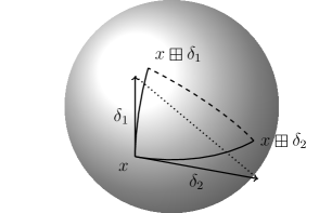
Figure 3: Axiom (11d): The $\mathrm{d}$-distance between $x\mathbin{\text{\raisebox{-0.86108pt}{$\boxplus$}}}\delta_{1}$ and $x\mathbin{\text{\raisebox{-0.86108pt}{$\boxplus$}}}\delta_{2}$ (dashed line) is less or equal to the distance in the parameterized around $x$ (dotted line).

The definition of the covariance of a $\mathbin{\text{\raisebox{-0.86108pt}{$\boxplus$}}}$-manifold distribution, on the other hand, is straightforward. As in the $\mathbb{R}^{n}$ case, it is an $n\times n$ matrix. Specifically, given a mean value $\operatorname{\operatorname{E}}X$ of a distribution $X:\Omega\to\mathcal{S}$, we define its covariance as

$$\operatorname{\operatorname{Cov}}X=\operatorname{\operatorname{E}}\left((X\mathbin{\text{\raisebox{-0.86108pt}{$\boxminus$}}}\operatorname{\operatorname{E}}X)(X\mathbin{\text{\raisebox{-0.86108pt}{$\boxminus$}}}\operatorname{\operatorname{E}}X)^{\top}\right),$$ (20)

because $X\mathbin{\text{\raisebox{-0.86108pt}{$\boxminus$}}}\operatorname{\operatorname{E}}X\in\mathbb{R}^{n}$ and the standard definition can be applied.

The $\mathbin{\text{\raisebox{-0.86108pt}{$\boxminus$}}}$-operator induces a metric (proof in App. A)

$$\mathrm{d}(x,y):=\left\|y\mathbin{\text{\raisebox{-0.86108pt}{$\boxminus$}}}x\right\|$$ (21)

that is important in interpreting $\operatorname{\operatorname{Cov}}X$. First,

$$\operatorname{tr}\operatorname{\operatorname{Cov}}X=\operatorname{\operatorname{E}}\left(\mathrm{d}(X,\operatorname{\operatorname{E}}X)^{2}\right).$$ (22)

i.e. $\sqrt{\operatorname{tr}\operatorname{\operatorname{Cov}}X}$ is the rms $\mathrm{d}$-distance of $X$ to the mean. Second, the states $y\in\mathcal{S}$ with $\mathrm{d}(\mu,y)=\sigma$ are the $1\sigma$ contour of $\operatorname{\mathcal{N}}(\mu,\sigma^{2}\operatorname{I})$. Hence, to interpret the state covariance or to define measurement or dynamic noise for a sensor fusion algorithm intuitively it is important that the metric induced by $\mathbin{\text{\raisebox{-0.86108pt}{$\boxminus$}}}$ has an intuitive meaning. For the $\mathbin{\text{\raisebox{-0.86108pt}{$\boxplus$}}}$-manifold representing orientation in the INS example, $\mathrm{d}(x,y)$ will be the angle between two orientations $x$ and $y$.

In the light of (21), axiom (11d) means that the actual distance $\mathrm{d}(x\mathbin{\text{\raisebox{-0.86108pt}{$\boxplus$}}}\delta_{1},x\mathbin{\text{\raisebox{-0.86108pt}{$\boxplus$}}}\delta_{2})$ is less or equal to the distance $\|\delta_{1}-\delta_{2}\|$ in the parametrization (Fig. 3), i.e. the map $x\mapsto x\mathbin{\text{\raisebox{-0.86108pt}{$\boxplus$}}}\delta$ is $1$-Lipschitz. This axiom is needed for all concepts explained in this subsection, as can be seen in the proofs in Appendix A. In so far, (11d) is the deepest insight in the axiomatization (11).

Appendix A also discusses a slight inconsistency in the definitions above, where the covariance of $\operatorname{\mathcal{N}}(\mu,\Sigma)$ defined by (13) and (20) is slightly smaller than $\Sigma$. For the usual case that $\Sigma$ is significantly smaller than the range of unique parameters $V$ (i.e. for angles $\ll\pi$), these inconsistencies are very small and can be practically ignored.

3.6 Practically Important $\mathbin{\text{\raisebox{-0.86108pt}{$\boxplus$}}}$-Manifolds

We will now define $\mathbin{\text{\raisebox{-0.86108pt}{$\boxplus$}}}$-operators for the practically most relevant manifolds $\mathbb{R}^{n}$ as well as 2D and 3D orientations. Appendix B proves the ones listed here to fulfill the axioms (11), Appendices A.5 and A.6 derive general techniques for constructing a $\mathbin{\text{\raisebox{-0.86108pt}{$\boxplus$}}}$-operator.

3.6.1 Vectorspace ($\mathbb{R}^{n}$)

For $\mathcal{S}=\mathbb{R}^{n}$, the $\mathbin{\text{\raisebox{-0.86108pt}{$\boxplus$}}}$- and $\mathbin{\text{\raisebox{-0.86108pt}{$\boxminus$}}}$-operators are, of course, simple vector addition and subtraction

$$x\mathbin{\text{\raisebox{-0.86108pt}{$\boxplus$}}}\delta=x+\delta,\quad y\mathbin{\text{\raisebox{-0.86108pt}{$\boxminus$}}}{}x=y-x.$$ (23)

3.6.2 2D Orientation as Angles Modulo $2\pi$

A planar rotation is the simplest case that requires taking its manifold structure into account. It can be represented by the rotation angle interpreted modulo $2\pi$. Mathematically, this is $\mathcal{S}=\mathbb{R}/2\pi\mathbb{Z}$, a set of equivalence classes. Practically, simply a real number $\alpha\in\mathbb{R}$ is stored, and periodic equivalents $\alpha+2\pi{}k,k\in\mathbb{Z}$ are treated as the same. $\mathbin{\text{\raisebox{-0.86108pt}{$\boxplus$}}}$ is, then, simply plus. It could be normalized but that is not necessary. The difference in $\mathbin{\text{\raisebox{-0.86108pt}{$\boxminus$}}}$ however, being a plain real value, must be normalized to $[-\pi,\pi)$ using a function $\nu_{\pi}$:

$$\begin{split}\alpha\mathbin{\text{\raisebox{-0.86108pt}{$\boxplus$}}}\delta=\alpha+\delta,\quad\beta\mathbin{\text{\raisebox{-0.86108pt}{$\boxminus$}}}\alpha=\nu_{\pi}(\beta-\alpha),\\ \text{where }\nu_{\pi}(\delta):=\delta-2\pi\left\lfloor\tfrac{\delta+\pi}{2\pi}\right\rfloor\end{split}$$ (24)

With this definition, $\beta\mathbin{\text{\raisebox{-0.86108pt}{$\boxminus$}}}\alpha$ is the smallest angle needed to rotate $\alpha$ into $\beta$, respecting the periodic interpretation of angles and giving the induced metric $\mathrm{d}(x,y)$ an intuitive meaning. The parametrization is unique for angles of modulus $<\pi$, i.e. $V=(-\pi,\pi)$.

3.6.3 3D Orientation as an Orthonormal Matrix

Rotations in 3D can be readily represented using orthonormal matrices $\mathcal{S}\subset\mathbb{R}^{3\times 3}$ with determinant $1$. $x\mathbin{\text{\raisebox{-0.86108pt}{$\boxplus$}}}\delta$ performs a rotation around axis $\delta$ in $x$ coordinates with angle $\left\|\delta\right\|$. This is also called matrix exponential representation and implemented by the Rodriguez formula [23, pp. 147]

$$x\mathbin{\text{\raisebox{-0.86108pt}{$\boxplus$}}}{}\delta=x\exp\delta,\quad y\mathbin{\text{\raisebox{-0.86108pt}{$\boxminus$}}}{}x=\log\left(x^{-1}y\right),$$ (25)

$$\begin{split}\exp\left[\begin{smallmatrix}x\\ y\\ z\end{smallmatrix}\right]=\left[\begin{smallmatrix}\cos\theta+cx^{2}&-sz+cxy&sy+cxz\\ sz+cxy&\cos\theta+cy^{2}&-sx+cyz\\ -sy+cxz&sx+cyz&\cos\theta+cz^{2}\end{smallmatrix}\right],\\ \theta=\sqrt{x^{2}+y^{2}+z^{2}},s=\operatorname{sinc}\theta,c=\tfrac{1-\cos\theta}{\theta^{2}}\end{split}$$ (26)

$$\log x=\frac{\theta}{2\sin\theta}\;\left[\begin{smallmatrix}x_{32}-x_{23}\\ x_{13}-x_{31}\\ x_{21}-x_{12}\end{smallmatrix}\right],\theta=\operatorname{acos}\tfrac{\operatorname{tr}x-1}{2}.$$ (27)

The induced metric $\mathrm{d}(x,y)$ is the angle of a rotation necessary to rotate $x$ onto $y$. There is also a monotonic relation to the widely used Frobenius distance $\left\|x-y\right\|_{\mathrm{F}}$ (Lemma 135, App. C). The parametrization is again unique for angles $<\pi$, i.e. $V=B_{\pi}(0)$, where, as usual, we denote by

$$B_{\varepsilon}(v)=\left\{w\in\mathbb{R}^{n}\mid\left\|w-v\right\|<\varepsilon\right\}$$ (28)

the open $\varepsilon$-ball around $v\in\mathbb{R}^{n}$ for $\varepsilon>0$.

3.6.4 3D Orientation as a Unit Quaternion

The same geometrical construction of rotating around $\delta$ by $\left\|\delta\right\|$ also works with unit quaternions $\mathcal{S}\subset\mathbb{H}$, where $q$ and $-q$ are considered equivalent as they represent the same orientation.

$$q\mathbin{\text{\raisebox{-0.86108pt}{$\boxplus$}}}\delta =q\cdot\exp\tfrac{\delta}{2},\;\;q\mathbin{\text{\raisebox{-0.86108pt}{$\boxminus$}}}p=2\operatorname{\overline{\log}}(p^{-1}\cdot q),$$ (29)

$$\exp\delta =\mathchoice{\left[\begin{matrix}\cos\left\|\delta\right\|\\ \operatorname{sinc}\left\|\delta\right\|\delta\end{matrix}\right]}{\bigl{[}\!\begin{smallmatrix}\cos\left\|\delta\right\|\\ \operatorname{sinc}\left\|\delta\right\|\delta\end{smallmatrix}\!\bigr{]}}{\bigl{[}\!\begin{smallmatrix}\cos\left\|\delta\right\|\\ \operatorname{sinc}\left\|\delta\right\|\delta\end{smallmatrix}\!\bigr{]}}{\bigl{[}\!\begin{smallmatrix}\cos\left\|\delta\right\|\\ \operatorname{sinc}\left\|\delta\right\|\delta\end{smallmatrix}\!\bigr{]}},$$ (30)

$$\operatorname{\overline{\log}}\mathchoice{\left[\begin{matrix}w\\ v\end{matrix}\right]}{\bigl{[}\!\begin{smallmatrix}w\\ v\end{smallmatrix}\!\bigr{]}}{\bigl{[}\!\begin{smallmatrix}w\\ v\end{smallmatrix}\!\bigr{]}}{\bigl{[}\!\begin{smallmatrix}w\\ v\end{smallmatrix}\!\bigr{]}} =\begin{cases}0&v=0\\ \tfrac{\operatorname{atan}(\left\|v\right\|/w)}{\left\|v\right\|}v&v\neq 0,w\neq 0\\ \pm\tfrac{\pi/2}{\left\|v\right\|}v&w=0.\end{cases}$$ (31)

The factor $2$ is introduced so that the induced metric $\mathrm{d}(p,q)$ is the angle between two orientations and the quaternion and matrix $\mathbin{\text{\raisebox{-0.86108pt}{$\boxplus$}}}$-manifolds are isomorphic. It originates from the fact that the quaternion is multiplied to the left and right of a vector when applying a rotation. The equivalence of $\pm q$ causes the $\operatorname{atan}(\left\|v\right\|/w)$ term in (31) instead of $\operatorname{atan2}(\left\|v\right\|,w)$, making $\operatorname{\overline{\log}}q=\operatorname{\overline{\log}}(-q)$.

3.6.5 Compound $\mathbin{\text{\raisebox{-0.86108pt}{$\boxplus$}}}$-Manifolds

Two (or several) $\mathbin{\text{\raisebox{-0.86108pt}{$\boxplus$}}}$-manifolds $\mathcal{S}_{1}$, $\mathcal{S}_{2}$ can be combined into a single $\mathbin{\text{\raisebox{-0.86108pt}{$\boxplus$}}}$-manifold by simply taking the Cartesian product $\mathcal{S}=\mathcal{S}_{1}\times\mathcal{S}_{2}$ and defining the $\mathbin{\text{\raisebox{-0.86108pt}{$\boxplus$}}}$- and $\mathbin{\text{\raisebox{-0.86108pt}{$\boxminus$}}}$-operator component-wise as

$$(x_{1},x_{2})\mathbin{\text{\raisebox{-0.86108pt}{$\boxplus$}}}\left[\begin{smallmatrix}\delta_{1}\\ \delta_{2}\end{smallmatrix}\right] :=(x_{1}\mathbin{\text{\raisebox{-0.86108pt}{$\boxplus$}}}_{\mathcal{S}_{1}}\delta_{1},x_{2}\mathbin{\text{\raisebox{-0.86108pt}{$\boxplus$}}}_{\mathcal{S}_{2}}\delta_{2})$$ (32)

$$(y_{1},y_{2})\mathbin{\text{\raisebox{-0.86108pt}{$\boxminus$}}}(x_{1},x_{2}) :=\left[\begin{smallmatrix}y_{1}\mathbin{\text{\raisebox{-0.60275pt}{$\boxminus$}}}_{\mathcal{S}_{1}}x_{1}\\ y_{2}\mathbin{\text{\raisebox{-0.60275pt}{$\boxminus$}}}_{\mathcal{S}_{2}}x_{2}\end{smallmatrix}\right].$$ (33)

4 Least Squares Optimization and Kalman Filtering on $\mathbin{\text{\raisebox{-0.86108pt}{$\boxplus$}}}$-Manifolds

Classical Gauss-Newton Gauss-Newton on a $$\mathbin{\text{\raisebox{-0.86108pt}{$\boxplus$}}}$$-Manifold

$$f:\mathbb{R}^{n}\to\mathbb{R}^{m} f:\mathcal{S}\to\mathcal{M}$$ (35)

$$f(X) \sim\operatorname{\mathcal{N}}\!\left(z,\,\Sigma\right)\Leftrightarrow f(X)-z\sim\operatorname{\mathcal{N}}\!\left(0,\,\Sigma\right) f(X) \sim z\mathbin{\text{\raisebox{-0.86108pt}{$\boxplus$}}}\operatorname{\mathcal{N}}\!\left(0,\,\Sigma\right)\stackrel{{\scriptstyle*}}{{\Leftrightarrow}}f(X)\mathbin{\text{\raisebox{-0.86108pt}{$\boxminus$}}}z\sim\operatorname{\mathcal{N}}\!\left(0,\,\Sigma\right)$$ (36)

Iterate with initial guess $$x_{0} x_{i}$$ until converges:

$$J_{\bullet k} :=\frac{f(x_{i}+\varepsilon e_{k})-f(x_{i}-\varepsilon e_{k})}{2\varepsilon} J_{\bullet k} :=\frac{(f(x_{i}\mathbin{\text{\raisebox{-0.86108pt}{$\boxplus$}}}\varepsilon e_{k})\mathbin{\text{\raisebox{-0.86108pt}{$\boxminus$}}}z)-(f(x_{i}\mathbin{\text{\raisebox{-0.86108pt}{$\boxplus$}}}-\varepsilon e_{k})\mathbin{\text{\raisebox{-0.86108pt}{$\boxminus$}}}z)}{2\varepsilon}$$ (37)

$$x_{i+1} :=x_{i}-(J^{\top}\Sigma^{-1}J)^{-1}J^{\top}\Sigma^{-1}(f(x_{i})-z) x_{i+1} :=x_{i}\mathbin{\text{\raisebox{-0.86108pt}{$\boxplus$}}}-(J^{\top}\Sigma^{-1}J)^{-1}J^{\top}\Sigma^{-1}(f(x_{i})\mathbin{\text{\raisebox{-0.86108pt}{$\boxminus$}}}z)$$ (38)

Table 1: Only small changes are necessary to adapt a classical least squares algorithm (left column) to work on $\mathbin{\text{\raisebox{-0.86108pt}{$\boxplus$}}}$-manifolds (right column). Adding perturbations to the state is done using $\mathbin{\text{\raisebox{-0.86108pt}{$\boxplus$}}}$, comparing values in the measurement space is done using $\mathbin{\text{\raisebox{-0.86108pt}{$\boxminus$}}}$. Note that the $\mathbin{\text{\raisebox{-0.86108pt}{$\boxminus$}}}z$ term does not cancel out when calculating the Jacobian. Also note that the equivalence marked by ^∗ holds only approximately, as we will derive in Appendix A.9.

One of the goals of the $\mathbin{\text{\raisebox{-0.86108pt}{$\boxplus$}}}$-method was to easily adapt estimation algorithms to work on arbitrary manifolds. Essentially, this can be done by replacing $+$ with $\mathbin{\text{\raisebox{-0.86108pt}{$\boxplus$}}}$ when adding perturbations to a state, and replacing $-$ with $\mathbin{\text{\raisebox{-0.86108pt}{$\boxminus$}}}$ when comparing two states or measurements. However, some pitfalls may arise, which we will deal with in this section.

We show how the $\mathbin{\text{\raisebox{-0.86108pt}{$\boxplus$}}}$-method can be applied to convert least squares optimization algorithms and the Unscented Kalman Filter such that they can operate on $\mathbin{\text{\raisebox{-0.86108pt}{$\boxplus$}}}$-manifolds rather than just $\mathbb{R}^{n}$.

4.1 Least Squares Optimization

Least squares optimization dates back to the late 18th century where it was used to combine measurements in astronomy and in geodesy. Initial publications were made by Legendre [29] and Gauss [12] in the early 19th century. The method is commonly used to solve overdetermined problems, i.e. problems having more “equations” or measurements than unknown variables.

When combining all unknowns into a single state $X\in\mathbb{R}^{n}$, and all measurement functions into a single function $f:\mathbb{R}^{n}\to\mathbb{R}^{m}$, the basic idea is to find $X$ such that given a combined measurement $z$,

$$\tfrac{1}{2}\left\|f(X)-z\right\|^{2}=\min!$$ (39)

(where we write “$=\min!$” to denote that the left-hand side becomes minimal). For a positive definite covariance $\Sigma$ between the measurements, this becomes

$$\tfrac{1}{2}\left\|f(X)-z\right\|_{\Sigma}^{2}=\min!$$ (40)

using the notation $\left\|x\right\|^{2}_{\Sigma}:=x^{\top}\Sigma^{-1}x$. Under the assumption that $f(X)=z+\varepsilon$, with $\varepsilon\sim\operatorname{\mathcal{N}}\!\left(0,\,\Sigma\right)$, this leads to a maximum likelihood solution.

If now our measurement function $f:\mathcal{S}\to\mathcal{M}$ maps from a state manifold $\mathcal{S}$ to a measurement manifold $\mathcal{M}$, we can write analogously:

$$\tfrac{1}{2}\left\|f(X)\mathbin{\text{\raisebox{-0.86108pt}{$\boxminus$}}}z\right\|_{\Sigma}^{2}=\min!$$ (41)

which again leads to a maximum likelihood solution, for $f(X)\mathbin{\text{\raisebox{-0.86108pt}{$\boxminus$}}}z\sim\operatorname{\mathcal{N}}\!\left(0,\,\Sigma\right)$, as we will prove in Appendix A.9.

Even for classical least squares problems, nonlinear functions $f$ usually allow only local, iterative solutions, i.e. starting from an initial guess $x_{0}$ we construct a sequence of approximations $x_{i}$ by calculating a refinement $\delta_{i}$ such that $x_{i+1}=x_{i}+\delta_{i}$ is a better solution than $x_{i}$.

This approach can be adapted to the manifold case, where every iteration takes place on a new local function

$$f_{x_{i}}^{z}:\mathbb{R}^{n} \to\mathbb{R}^{m}$$ (42)

$$\delta \mapsto f(x_{i}\mathbin{\text{\raisebox{-0.86108pt}{$\boxplus$}}}\delta)\mathbin{\text{\raisebox{-0.86108pt}{$\boxminus$}}}z,$$ (43)

which for smooth $f$ is a smooth function and, as it is an ordinary vector function, a local refinement $\delta_{i}$ can be found analogously to the classical case. This refinement can then be added to the previous state using $x_{i+1}:=x_{i}\mathbin{\text{\raisebox{-0.86108pt}{$\boxplus$}}}\delta_{i}$. The key difference is that now the refinements are accumulated in $\mathcal{S}$, not in $\mathbb{R}^{n}$. In Table 1 we show how this can be done using the popular Gauss-Newton method with finite-difference Jacobian calculation. Other least squares methods like Levenberg-Marquardt can be applied analogously.

4.2 Kalman Filtering

Since its inception in the late 1950s, the Kalman filter [20] and its many variants have successfully been applied to a wide variety of state estimation and control problems. In its original form, the Kalman filter provides a framework for continuous state and discrete time state estimation of linear Gaussian systems. Many real-world problems, however, are intrinsically non-linear, which gives rise to the idea of modifying the Kalman filter algorithm to work with non-linear process models (mapping old to new state) and measurement models (mapping state to expected measurements) as well.

The two most popular extensions of this kind are the Extended Kalman Filter (EKF) [4, Chap. 5.2] and more recently the Unscented Kalman Filter (UKF) [18]. The EKF linearizes the process and measurement models through first order Taylor series expansion. The UKF, on the other hand, is based on the unscented transform which approximates the respective probability distributions through deterministically chosen samples, so-called sigma points, propagates these directly through the non-linear process and measurement models and recovers the statistics of the transformed distribution from the transformed samples. Thus, intuitively, the EKF relates to the UKF as a tangent to a secant.

We will focus on the UKF here since it is generally better at handling non-linearities and does not require (explicit or numerically approximated) Jacobians of the process and measurement models, i.e. it is a derivative-free filter. Although the UKF is fairly new, it has been used successfully in a variety of robotics applications ranging from ground robots [41] to unmanned aerial vehicles (UAVs) [33].

The UKF algorithm has undergone an evolution from early publications on the unscented transform [36] to the work by Julier and Uhlmann [17, 18] and by van der Merwe et al. [32, 33]. The following is based on the consolidated UKF formulation by Thrun, Burgard & Fox [40] with parameters chosen as discussed in [43]. The modification of the UKF algorithm for use with manifolds is based on [11], [25], [5] and [43].

4.2.1 Non-Linear Process and Measurement Models

UKF process and measurement models need not be linear but are assumed to be subject to additive white Gaussian noise, i.e.

$$x_{t} =g(u_{t},x_{t-1})+\varepsilon_{t}$$ (44)

$$z_{t} =h(x_{t})+\delta_{t}$$ (45)

where $g:T\times\mathbb{R}^{n}\to\mathbb{R}^{n}$ and $h:\mathbb{R}^{n}\to\mathbb{R}^{m}$ are arbitrary (but sufficiently nice) functions, $T$ is the space of controls, $\varepsilon_{t}\sim\operatorname{\mathcal{N}}\!\left(0,\,R_{t}\right)$, $\delta_{t}\sim\operatorname{\mathcal{N}}\!\left(0,\,Q_{t}\right)$, and all $\varepsilon_{t}$ and $\delta_{t}$ are independent.

4.2.2 Sigma Points

The set of $2n+1$ sigma points that are used to approximate an $n$-dimensional Gaussian distribution with mean $\mu$ and covariance $\Sigma$ is computed as follows:

$$\mathcal{X}^{[0]} =\mu$$ (46)

$$\mathcal{X}^{[i]} =\mu+\bigl{(}\sqrt{\Sigma}\bigr{)}_{\bullet i}\text{ for }i=1,\ldots,n$$ (47)

$$\mathcal{X}^{[i+n]} =\mu-\bigl{(}\sqrt{\Sigma}\bigr{)}_{\bullet i}\text{ for }i=1,\ldots,n$$ (48)

where $\bigl{(}\sqrt{\Sigma}\bigr{)}_{\bullet i}$ denotes the $i$-th column of a matrix square root $\sqrt{\Sigma}\sqrt{\Sigma}^{T}=\Sigma$ implemented by Cholesky decomposition. The name sigma points reflects the fact that all $\mathcal{X}^{[k]}$ lie on the $1\sigma$-contour for $k>0$.

In the following we will use the abbreviated notation

$$\mathcal{X}=(\mu\hskip 28.45274pt\mu+\sqrt{\Sigma}\hskip 28.45274pt\mu-\sqrt{\Sigma})$$ (49)

to describe the generation of the sigma points.

4.2.3 Modifying the UKF Algorithm for Use with $\mathbin{\text{\raisebox{-0.86108pt}{$\boxplus$}}}$-Manifolds

The complete UKF algorithm is given in Table 2.

Classical UKF UKF on $$\mathbin{\text{\raisebox{-0.86108pt}{$\boxplus$}}}$$-Manifolds

Input, Process and Measurement Models:

$$\mu_{t-1} \in\mathbb{R}^{n},\Sigma_{t-1}\in\mathbb{R}^{n\times n},u_{t}\in T,z_{t}\in\mathbb{R}^{m} \mu_{t-1} \in\mathcal{S},\Sigma_{t-1}\in\mathbb{R}^{n\times n},u_{t}\in T,z_{t}\in\mathcal{M}$$ (51)

$$g :T\!\times\!\mathbb{R}^{n}\to\!\mathbb{R}^{n},X_{t}\!=\!g(u_{t},X_{t-1})+\operatorname{\mathcal{N}}(0,R_{t}) g :T\!\times\!\mathcal{S}\to\!\mathcal{S},X_{t}\!=\!g(u_{t},X_{t-1})\mathbin{\text{\raisebox{-0.86108pt}{$\boxplus$}}}\operatorname{\mathcal{N}}(0,R_{t})$$ (52)

$$h :\mathbb{R}^{n}\to\mathbb{R}^{m},z_{t}=h(X_{t})+\operatorname{\mathcal{N}}(0,Q_{t}) h :\mathcal{S}\to\mathcal{M},z_{t}=h(X_{t})\mathbin{\text{\raisebox{-0.86108pt}{$\boxplus$}}}_{\mathcal{M}}\operatorname{\mathcal{N}}(0,Q_{t})$$ (53)

Prediction Step:

$$\mathcal{X}_{t-1} =(\mu_{t-1}\hskip 7.11317pt\mu_{t-1}+\sqrt{\Sigma_{t-1}}\hskip 7.11317pt\mu_{t-1}-\sqrt{\Sigma_{t-1}}) \mathcal{X}_{t-1} =(\mu_{t-1}\hskip 7.11317pt\mu_{t-1}\mathbin{\text{\raisebox{-0.86108pt}{$\boxplus$}}}\sqrt{\Sigma_{t-1}}\hskip 7.11317pt\mu_{t-1}\mathbin{\text{\raisebox{-0.86108pt}{$\boxplus$}}}-\sqrt{\Sigma_{t-1}})$$ (54)

$$\bar{\mathcal{X}}_{t}^{*} =g(u_{t},\mathcal{X}_{t-1}) \bar{\mathcal{X}}_{t}^{*} =g(u_{t},\mathcal{X}_{t-1})$$ (55)

$$\bar{\mu}_{t} =\frac{1}{2n+1}\sum_{i=0}^{2n}\bar{\mathcal{X}}_{t}^{*[i]} \bar{\mu}_{t} =\mbox{\sc MeanOfSigmaPoints}(\bar{\mathcal{X}}_{t}^{*})$$ (56)

$$\bar{\Sigma}_{t} =\frac{1}{2}\sum_{i=0}^{2n}(\bar{\mathcal{X}}_{t}^{*[i]}-\bar{\mu}_{t})(\bar{\mathcal{X}}_{t}^{*[i]}-\bar{\mu}_{t})^{\top}+R_{t} \bar{\Sigma}_{t} =\frac{1}{2}\sum_{i=0}^{2n}(\bar{\mathcal{X}}_{t}^{*[i]}\mathbin{\text{\raisebox{-0.86108pt}{$\boxminus$}}}\bar{\mu}_{t})(\bar{\mathcal{X}}_{t}^{*[i]}\mathbin{\text{\raisebox{-0.86108pt}{$\boxminus$}}}\bar{\mu}_{t})^{\top}+R_{t}$$ (57)

Correction Step:

$$\bar{\mathcal{X}}_{t} =(\bar{\mu}_{t}\hskip 14.22636pt\bar{\mu}_{t}+\sqrt{\bar{\Sigma}_{t}}\hskip 14.22636pt\bar{\mu}_{t}-\sqrt{\bar{\Sigma}_{t}}) \bar{\mathcal{X}}_{t} =(\bar{\mu}_{t}\hskip 14.22636pt\bar{\mu}_{t}\mathbin{\text{\raisebox{-0.86108pt}{$\boxplus$}}}\sqrt{\bar{\Sigma}_{t}}\hskip 14.22636pt\bar{\mu}_{t}\mathbin{\text{\raisebox{-0.86108pt}{$\boxplus$}}}-\sqrt{\bar{\Sigma}_{t}})$$ (58)

$$\bar{\mathcal{Z}}_{t} =h(\bar{\mathcal{X}}_{t}) \bar{\mathcal{Z}}_{t} =h(\bar{\mathcal{X}}_{t})$$ (59)

$$\hat{z}_{t} =\frac{1}{2n+1}\sum_{i=0}^{2n}\bar{\mathcal{Z}}_{t}^{[i]} \hat{z}_{t} =\mbox{\sc MeanOfSigmaPoints}(\bar{\mathcal{Z}}_{t})$$ (60)

$$S_{t} =\frac{1}{2}\sum_{i=0}^{2n}(\bar{\mathcal{Z}}_{t}^{[i]}-\hat{z}_{t})(\bar{\mathcal{Z}}_{t}^{[i]}-\hat{z}_{t})^{\top}+Q_{t} S_{t} =\frac{1}{2}\sum_{i=0}^{2n}(\bar{\mathcal{Z}}_{t}^{[i]}\mathbin{\text{\raisebox{-0.86108pt}{$\boxminus$}}}_{\mathcal{M}}\hat{z}_{t})(\bar{\mathcal{Z}}_{t}^{[i]}\mathbin{\text{\raisebox{-0.86108pt}{$\boxminus$}}}_{\mathcal{M}}\hat{z}_{t})^{\top}+Q_{t}$$ (61)

$$\bar{\Sigma}_{t}^{x,z} =\frac{1}{2}\sum_{i=0}^{2n}(\bar{\mathcal{X}}_{t}^{[i]}-\bar{\mu}_{t})(\bar{\mathcal{Z}}_{t}^{[i]}-\hat{z}_{t})^{\top} \bar{\Sigma}_{t}^{x,z} =\frac{1}{2}\sum_{i=0}^{2n}(\bar{\mathcal{X}}_{t}^{[i]}\mathbin{\text{\raisebox{-0.86108pt}{$\boxminus$}}}\bar{\mu}_{t})(\bar{\mathcal{Z}}_{t}^{[i]}\mathbin{\text{\raisebox{-0.86108pt}{$\boxminus$}}}_{\mathcal{M}}\hat{z}_{t})^{\top}$$ (62)

$$K_{t} =\bar{\Sigma}_{t}^{x,z}S_{t}^{-1} K_{t} =\bar{\Sigma}_{t}^{x,z}S_{t}^{-1}$$ (63)

$$\mu_{t} =\bar{\mu}_{t}+K_{t}(z_{t}-\hat{z}_{t}) \delta =K_{t}(z_{t}\mathbin{\text{\raisebox{-0.86108pt}{$\boxminus$}}}_{\mathcal{M}}\hat{z}_{t})$$ (64)

$$\Sigma_{t} =\bar{\Sigma}_{t}-K_{t}S_{t}K_{t}^{\top} \Sigma_{t}^{\prime} =\bar{\Sigma}_{t}-K_{t}S_{t}K_{t}^{\top}$$ (65)

$$\mathcal{X}_{t}^{\prime} =(\bar{\mu}_{t}\mathbin{\text{\raisebox{-0.86108pt}{$\boxplus$}}}\delta\hskip 7.11317pt\bar{\mu}_{t}\mathbin{\text{\raisebox{-0.86108pt}{$\boxplus$}}}(\delta+\sqrt{\Sigma_{t}^{\prime}})\hskip 7.11317pt\bar{\mu}_{t}\mathbin{\text{\raisebox{-0.86108pt}{$\boxplus$}}}(\delta-\sqrt{\Sigma_{t}^{\prime}}))$$ (66)

$$\mu_{t} =\mbox{\sc MeanOfSigmaPoints}(\mathcal{X}_{t}^{\prime})$$ (67)

$$\Sigma_{t} =\frac{1}{2}\sum_{i=0}^{2n}(\mathcal{X}_{t}^{\prime[i]}\mathbin{\text{\raisebox{-0.86108pt}{$\boxminus$}}}\mu_{t})(\mathcal{X}_{t}^{\prime[i]}\mathbin{\text{\raisebox{-0.86108pt}{$\boxminus$}}}\mu_{t})^{\top}$$ (68)

Table 2: Classical UKF vs. UKF on $\mathbin{\text{\raisebox{-0.86108pt}{$\boxplus$}}}$-manifolds algorithms. See text for details.

Like other Bayes filter instances, it consists of two alternating steps – the prediction and the correction step. The prediction step of the UKF takes the previous belief represented by its mean $\mu_{t-1}$ and covariance $\Sigma_{t-1}$ and a control $u_{t}$ as input, calculates the corresponding set of sigma points, applies the process model to each sigma point, and recovers the statistics of the transformed distribution as the predicted belief with added process noise $R_{t}$ ((54) to (57)).

To convert the prediction step of the UKF for use with $\mathbin{\text{\raisebox{-0.86108pt}{$\boxplus$}}}$-manifolds we need to consider operations that deal with states. These add a perturbation vector to a state in (54), determine the difference between two states in (57), and calculate the mean of a set of sigma points in (56). In the manifold case, perturbation vectors are added via $\mathbin{\text{\raisebox{-0.86108pt}{$\boxplus$}}}$ and the difference between two states is simply determined via $\mathbin{\text{\raisebox{-0.86108pt}{$\boxminus$}}}$. The mean of a set of manifold sigma points can be computed analogously to the definition of the expected value from (17) and (18); the definition of the corresponding function MeanOfSigmaPoints is shown in Table 3.

$$\mathbin{\text{\raisebox{-0.86108pt}{$\boxplus$}}}$$-Manifold-MeanOfSigmaPoints

Input:

$$\mathcal{Y}^{[i]}, \;\;i=0,\ldots,2n$$ (70)

Determine mean $$\mu^{\prime}$$:

$$\mu_{0}^{\prime} =\mathcal{Y}^{[0]}$$ (71)

$$\mu_{k+1}^{\prime} =\mu_{k}^{\prime}\mathbin{\text{\raisebox{-0.86108pt}{$\boxplus$}}}\frac{1}{2n+1}\sum_{i=0}^{2n}\mathcal{Y}^{[i]}\mathbin{\text{\raisebox{-0.86108pt}{$\boxminus$}}}\mu_{k}^{\prime}$$ (72)

$$\mu^{\prime} =\lim_{k\rightarrow\infty}\mu_{k}^{\prime}$$ (73)

Table 3: MeanOfSigmaPoints computes the mean of a set of $\mathbin{\text{\raisebox{-0.86108pt}{$\boxplus$}}}$-manifold sigma points $\mathcal{Y}$. In practice, the limit in (73) can be implemented by an iterative loop that is terminated if the norm of the most recent summed error vector is below a certain threshold. The number of sigma points is not necessarily the same as the dimension of each.

The UKF correction step first calculates the new set of sigma points (58), propagates each through the measurement model to obtain the sigma points corresponding to the expected measurement distribution in (59), and recovers its mean $\hat{z}_{t}$ in (60) and covariance $S_{t}$ with added measurement noise $Q_{t}$ in (61). Similarly, the cross-covariance $\bar{\Sigma}_{t}^{x,z}$ between state and expected measurement is calculated in (62). The latter two are then used in (63) to compute the Kalman gain $K$, which determines how the innovation is to be used to update the mean in (64) and how much uncertainty can be removed from the covariance matrix in (65) to reflect the information gained from the measurement.

The conversion of the UKF correction step for use with $\mathbin{\text{\raisebox{-0.86108pt}{$\boxplus$}}}$-manifolds generally follows the same strategy as that of the prediction step but is more involved in detail. Firstly, this is because we use $\mathbin{\text{\raisebox{-0.86108pt}{$\boxplus$}}}$-manifolds to represent both states and measurements so that the advantages introduced for states above also apply to measurements. Secondly, the update of the mean in (64) cannot be implemented as a simple application of $\mathbin{\text{\raisebox{-0.86108pt}{$\boxplus$}}}$: This might result in an inconsistency between the covariance matrix and the mean since in general

$$\mu\mathbin{\text{\raisebox{-0.86108pt}{$\boxplus$}}}\operatorname{\mathcal{N}}\!\left(\delta,\,\Sigma^{\prime}\right)\neq(\mu\mathbin{\text{\raisebox{-0.86108pt}{$\boxplus$}}}\delta)\mathbin{\text{\raisebox{-0.86108pt}{$\boxplus$}}}\operatorname{\mathcal{N}}\!\left(0,\,\Sigma^{\prime}\right),$$ (74)

i.e. the mean would be modified while the covariance is still formulated in terms of the coordinate system defined by the old mean as the reference point. Thus, we need to apply an additional sigma point propagation as follows. The manifold variant of (64) only determines the perturbation vector $\delta$ by which the mean is to be changed and the manifold variant of (65) calculates a temporary covariance matrix $\Sigma_{t}^{\prime}$ still relative to the old mean $\bar{\mu}_{t}$. (66) then adds the sum of $\delta$ and the respective columns of $\Sigma_{t}^{\prime}$ to $\bar{\mu}_{t}$ in a single $\mathbin{\text{\raisebox{-0.86108pt}{$\boxplus$}}}$ operation to generate the set of sigma points $\mathcal{X}_{t}^{\prime}$. Therefrom the new mean $\mu_{t}$ in (67) and covariance $\Sigma_{t}$ in (68) is computed.

The overhead of the additional sigma point propagation can be avoided by storing $\mathcal{X}_{t}^{\prime}$ for reuse in (54) or (58). If $x\mathbin{\text{\raisebox{-0.86108pt}{$\boxplus$}}}\delta$ is continuous in $x$, the step can also be replaced by $\mu_{t}=\bar{\mu}_{t}\mathbin{\text{\raisebox{-0.86108pt}{$\boxplus$}}}\delta$ as an approximation.

A final word auf caution: Sigma point propagation fails for a standard deviation larger than the range $V$ of unique parametrization, where even propagation through the identity function results in a reduced covariance. To prevent this, the standard deviation must be within $V/2$, so all sigma points are mutually within a range of $V$. For 2D and 3D orientation hence an angular standard deviation of $\pi/2$ is allowed. This is no practical limitation, because filters usually fail much earlier because of nonlinearity.

5 $\mathbin{\text{\raisebox{-0.86108pt}{$\boxplus$}}}$-Manifolds as a
Software Engineering Tool

As discussed in Section 3, the $\mathbin{\text{\raisebox{-0.86108pt}{$\boxplus$}}}$-method simultaneously provides two alternative views of a $\mathbin{\text{\raisebox{-0.86108pt}{$\boxplus$}}}$-manifold. On the one hand, generic algorithms access primitive or compound manifolds via flattened perturbation vectors, on the other hand, the user implementing process and measurement models needs direct access to the underlying state representation (such as a quaternion) and for compound manifolds wants to access individual components by a descriptive name.

In this section we will use our Manifold Toolkit (MTK) to illustrate how the $\mathbin{\text{\raisebox{-0.86108pt}{$\boxplus$}}}$-method can be modeled in software. The current version of MTK is implemented in C++ and uses the Boost Preprocessor library [2] and the Eigen Matrix library [15]. A port to MATLAB is also available [44]. Similar mechanisms can be applied in other (object-oriented) programming languages.

5.1 Representing Manifolds in Software

In MTK, we represent $\mathbin{\text{\raisebox{-0.86108pt}{$\boxplus$}}}$-manifolds as C++ classes and require every manifold to provide a common interface to be accessed by the generic sensor fusion algorithm, i.e. implementations of $\mathbin{\text{\raisebox{-0.86108pt}{$\boxplus$}}}$ and $\mathbin{\text{\raisebox{-0.86108pt}{$\boxminus$}}}$. The corresponding C++ interface is fairly straight-foward. Defining a manifold requires an enum DOF and two methods

⬇

struct MyManifold {

enum {DOF = $n$};

typedef double scalar;

void boxplus(vectview<const double, DOF> delta, double scale=1);

void boxminus(vectview<double, DOF> delta,

const MyManifold& other) const;

};

where $n$ is the degrees of freedom, x.boxplus(delta, s) implements $x:=x\mathbin{\text{\raisebox{-0.86108pt}{$\boxplus$}}}(s\cdot\delta)$ and y.boxminus(delta, x) implements $\delta:=y\mathbin{\text{\raisebox{-0.86108pt}{$\boxminus$}}}x$. vectview maps a double array of size DOF to an expression directly usable in Eigen expressions. The scaling factor in boxplus can be set to $-1$ to conveniently implement $x\mathbin{\text{\raisebox{-0.86108pt}{$\boxplus$}}}(-\delta)$.

Additionally, a $\mathbin{\text{\raisebox{-0.86108pt}{$\boxplus$}}}$-manifold class can provide arbitrary member variables and methods (which, e.g. rotate vectors in the case of orientation) that are specific to the particular manifold.

MTK already comes with a library of readily available manifold primitive implementations of $\mathbb{R}^{n}$ as vect<n>, $SO(2)$ and $SO(3)$ as SO2 and SO3 respectively, and $S^{2}$ as S2. It is possible to provide alternative implementations of these or to add new implementations of other manifolds basically by writing appropriate $\mathbin{\text{\raisebox{-0.86108pt}{$\boxplus$}}}$ and $\mathbin{\text{\raisebox{-0.86108pt}{$\boxminus$}}}$ methods.

5.2 Automatically Generated Compound Manifold Representations

In practice, a single manifold primitive is usually insufficient to represent states (or measurements). Thus, we also need to cover compound $\mathbin{\text{\raisebox{-0.86108pt}{$\boxplus$}}}$-manifolds consisting of several manifold components in software.

A user-friendly approach would encapsulate the manifold in a class with members for each individual submanifold which, mathematically, corresponds to a Cartesian product. Following this approach, $\mathbin{\text{\raisebox{-0.86108pt}{$\boxplus$}}}$/$\mathbin{\text{\raisebox{-0.86108pt}{$\boxminus$}}}$ operators on the compound manifold are needed, which use the $\mathbin{\text{\raisebox{-0.86108pt}{$\boxplus$}}}$/$\mathbin{\text{\raisebox{-0.86108pt}{$\boxminus$}}}$ operators of the components as described in Section 3.6.5. Using this method, the user can access members of the manifold by name, and the algorithm just sees the compound manifold.

This can be done by hand in principle, but becomes quite error-prone when there are many components. Therefore, MTK provides a preprocessor macro which generates a compound manifold from a list of simple manifolds. The way how MTK does this automatically and hides all details from the user is a main contribution of MTK.

Returning to the INS example from the introduction where we need to represent a state consisting of a position, an orientation, and a velocity, we would have a nine-degrees-of-freedom state

$$\mathcal{S}=\mathbb{R}^{3}\times SO(3)\times\mathbb{R}^{3}.$$ (75)

Using our toolkit this can be constructed as:

⬇

((vect<3>, pos))

((SO3, orient))

((vect<3>, vel))

)

Given this code snippet the preprocessor will generate a class state, having public members pos, orient, and vel. Also generated are the manifold operations boxplus and boxminus as well as the total degrees of freedom state::DOF = 9 of the compound manifold.

The macro also addresses another technical problem: Kalman filters in particular require covariance matrices to be specified which represent process and measurement noise. Similarly, individual parts of covariance matrices often need to be analyzed. In both cases the indices of individual components in the flattened vector view need to be known. MTK makes this possible by generating an enum IDX reflecting the index corresponding to the start of the respective part of the vector view. In the above example, the start of the vectorized orientation can be determined using e.g. s.orient.IDX for a state s. The size of this part is given by s.orient.DOF. MTK also provides convenience methods to access and modify corresponding sub-vectors or sub-matrices using member pointers.

⬇

Matrix<double, state::DOF, state::DOF> cov;

cov.setZero();

// set diagonal of covariance block of pos part:

setDiagonal(cov, &state::pos, 1);

// fill entire orient-pos-covariance block:

subblock(cov, &state::orient, &state::pos).fill(0.1);

5.3 Generic Least Squares Optimization and UKF Implementations

Based on MTK, we have developed a generic least squares optimization framework called SLoM (Sparse Least Squares on Manifolds) [16] according to Table 1 and UKFoM [43], a generic UKF on manifolds implementation according to Table 2. Apart from handling manifolds, SLoM automatically infers sparsity, i.e. which measurement depends on which variables, and exploits this in computing the Jacobian in (37), and in representing, and inverting it in (38).

MTK, SLoM and UKFoM are already available online on www.openslam.org/mtk under an open source license.

6 Experiments

We now illustrate the advantages of the $\mathbin{\text{\raisebox{-0.86108pt}{$\boxplus$}}}$-method in terms of both ease of use and algorithmic performance.

6.1 Worked Example: INS-GPS Integration

In a first experiment, we show how MTK and UKFoM can be used to implement a minimalistic, but working INS-GPS filter in about 50 lines of C++ code. The focus is on how the framework allows to concisely write down such a filter. It integrates accelerometer and gyroscope readings in the prediction step and fuses a global position measurement (e.g. loosely coupled GPS) in the measurement update. The first version assumes white noise. We then show how the framework allows for an easy extension to colored noise.

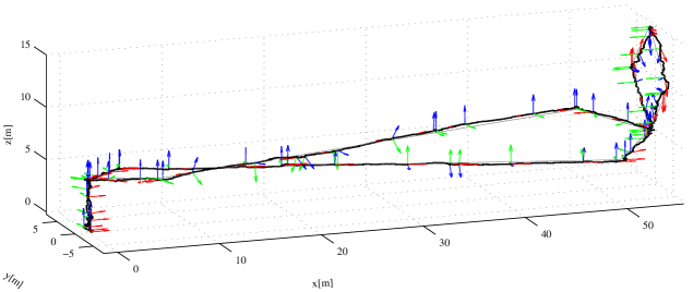
Figure 4: Trajectory estimated from a synthetic dataset by the UKFoM-based minimal INS-GPS filter. The trajectory starts and ends at $(0,0)$ and consists of a stylized figure eight with an embedded stylized loop (right). While on the long segments of the figure eight the helicopter rotates about its roll axis.

6.1.1 IMU Process Model

Reusing the state manifold definition from Section 5.2, the process model implements $x_{t}=g(u_{t},x_{t-1})$ (cf. Section 4.2.1) where the control $u_{t}$ in this case comprises acceleration a as measured by a three-axis accelerometer and angular velocity w as measured by a three-axis gyroscope.

⬇

const vect<3> &a, const vect<3> &w)

{

state s2;

// apply rotation

vect<3> scaled_axis = w * dt;

SO3 rot = SO3::exp(scaled_axis);

s2.orient = s.orient * rot;

// accelerate with gravity

s2.vel = s.vel + (s.orient * a + gravity) * dt;

// translate

s2.pos = s.pos + s.vel * dt;

return s2;

}

The body of the process model uses Euler integration of the motion described by a and w over a short time interval dt. Note how individual components of the manifold state are accessed by name and how they can provide non-trivial methods (overloaded operators).

Further, we need to implement a function that returns the process noise term $R_{t}$.

⬇

{

ukf<state>::cov cov = ukf<state>::cov::Zero();

setDiagonal(cov, &state::pos, 0);

setDiagonal(cov, &state::orient,gyro_noise*dt);

setDiagonal(cov, &state::vel, acc_noise*dt);

return cov;

}

Note how the MTK’s setDiagonal function automatically fills in the diagonal entries of the covariance matrix such that their order matches the way the $\mathbin{\text{\raisebox{-0.86108pt}{$\boxplus$}}}$/$\mathbin{\text{\raisebox{-0.86108pt}{$\boxminus$}}}$ operators locally vectorize the state space, i.e. the user does not need to know about these internals. The constants $\sigma_{\omega}^{2}=\;$gyro_noise and $\sigma_{v}^{2}=\;$acc_noise are continuous noise spectral densities for the gyroscope ($\tfrac{\text{rad}^{2}}{\text{s}}$) and accelerometer ($\tfrac{\text{m}^{2}}{\text{s}^{3}}$) and multiplied by dt in the process noise covariance matrix

$$R_{t}=dt\cdot\operatorname{diag}(0,0,0,\sigma_{\omega}^{2},\sigma_{\omega}^{2},\sigma_{\omega}^{2},\sigma_{v}^{2},\sigma_{v}^{2},\sigma_{v}^{2}).$$ (76)

6.1.2 GPS Measurement Model

Measurement models implement $z_{t}=h(x_{t})$ (cf. Section 4.2.1), in the case of a position measurement simply returning the position from $x_{t}$.

⬇

{

return s.pos;

}

We also need to implement a function that returns the measurement noise term $Q_{t}$.

⬇

{

return gpos_noise * Matrix3x3::Identity();

}

Again, $\sigma_{p}^{2}=\;$gps_noise is constant. Note that although we show a vector measurement in this example, UKFoM also supports manifold measurements.

6.1.3 Executing the Filter

Executing the UKF is now straight-forward. We first instantiate the ukf template with our state type and pass a default $(0,1,0)$ initial state to the constructor along with an initial covariance matrix. We then assume that sensor data is acquired in some form of loop, and at each iteration execute the prediction and correction (update) steps with the process and measurement models and sensor readings as arguments.

⬇

0.001 * ukf<state>::cov::Identity();

ukf<state> kf(state(), init_cov);

vect<3> acc, gyro, gps;

for (...)

{

kf.predict(

boost::bind(process_model, _1, acc, gyro),

process_noise_cov);

kf.update<3>(gps,

gps_measurement_model,

gps_measurement_noise_cov);

}

Note how our use of boost::bind denotes an anonymous function that maps the state _1 to process_model(_1, acc, gyro).

Also note that there is no particular order in which predict() and update() need to be called, and that there can be more than one measurement model – typically one per type of sensor data.

6.1.4 Evaluation on a Synthetic Dataset

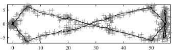
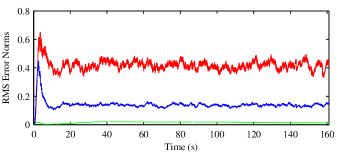
Figure 5: Top: Trajectory estimated by the minimal INS-GPS filter (black) vs. ground truth (solid gray) and position measurements (gray crosses) from a single filter run. The plot shows the $x$-$y$-plane (m). Bottom: RMS error norms for position (red, m), orientation (green, rad) and velocity (blue, m/s) estimates from 50 Monte Carlo runs. The time averaged error is $0.415\,m$, $1.58\times 10^{-2}\,rad$ and $0.141\,m/s$, respectively. This magnitude seems plausible for a $\sigma_{p}=0.75\,\text{m}$ GPS.

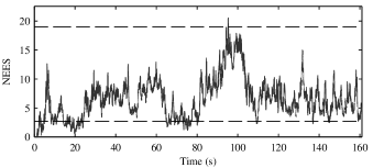
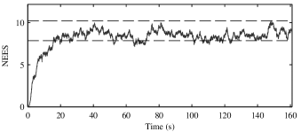
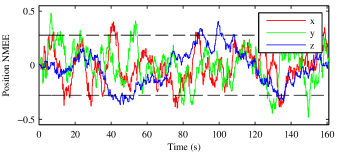
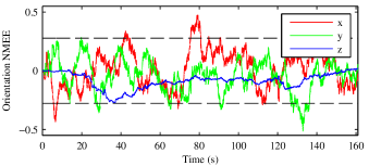
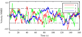
Figure 6: Plots for filter consistency evaluation (top to bottom): NEES $\left\|\mu_{t}\boxminus X_{t}\right\|_{\Sigma_{t}}^{2}$ from a single run; averaged NEES from 50 Monte Carlo runs; $\frac{(\mu_{t}\mathbin{\text{\raisebox{-0.60275pt}{$\boxminus$}}}X_{t})_{k}}{\sqrt{\Sigma_{tkk}}}$ averaged over 50 Monte Carlo runs (NMEE) with $k$ being x, y, and z of position, orientation and velocity . Note how each largely remains within its 95% probability region (dashed), as should be the case for a consistent filter.

To conclude the worked example, we run the filter on a synthetic data set consisting of sensor data generated from a predefined trajectory with added white Gaussian noise. The estimated 3D trajectory is shown in Figure 4, its projection into the $x$-$y$-plane compared to ground truth in Figure 5. Accelerometer and gyroscope readings are available at 100 Hz ($dt=0.01$) with white noise standard deviations $\sigma_{\omega}=0.05\degree/\text{s}^{1/2}$ and $\sigma_{v}=2\,\text{mm}/\text{s}^{3/2}$ (MEMS class IMU). GPS is available at 4 Hz, with white noise of $\sigma_{p}=0.75\,\text{m}$.

Solely based on accelerometer and gyroscope data the state estimate would drift over time. GPS measurements allow the filter to reset errors stemming from accumulated process noise. However, over short time periods accelerometer and gyroscope smooth out the noisy GPS measurements as illustrated in Figure 5. As suggested by [4] we verify the filter consistency by computing the normalized estimation error squared (NEES) and the normalized mean estimation error (NMEE) for each state component (Fig. 6). Figure 7 and 8 present the same results for a UKF using Euler angles and scaled axis respectively, showing the expected failure once the orientation approaches singularity. Figure 9 shows the results for the technique proposed in [33] with a plain quaternion $\mathbb{R}^{4}$ in the UKF state and a process model that drives the quaternion towards normalization ($\eta=0.1/\text{s}$, cf. Sec. 2.3). Overall, Euler-angle and scaled axis fail at singularities, the $\mathbin{\text{\raisebox{-0.86108pt}{$\boxplus$}}}$-method is very slightly better than the plain quaternion. The difference in performance is not very relevant, our claim is rather that the $\mathbin{\text{\raisebox{-0.86108pt}{$\boxplus$}}}$-method is conceptually more elegant. Computation time was 21/32 $\mu$s ($\mathbin{\text{\raisebox{-0.86108pt}{$\boxplus$}}}$), 28/23 $\mu$s (Euler), 25/23 $\mu$s (scaled axis), 21/33 $\mu$s (quaternion) for a predict-step/for a GPS update. All timings were determined on an Intel Xeon CPU E5420 @2.50GHz running 32bit Linux.

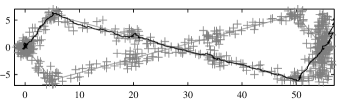
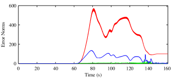
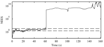
Figure 7: Performance of an UKF using Euler angles for the orientation (top to bottom): Trajectory estimated, error norms as in Fig. 5, NEES, from a single run. The filter operates normally until $t=60\,\text{s}$ where the orientation approaches the singularity, the filter becomes inconsistent and the error rapidly increases with the estimate leaving the workspace.

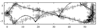
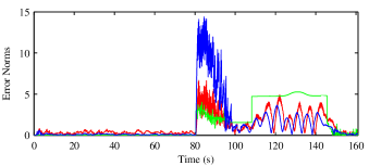
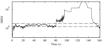
Figure 8: Performance of an UKF using a scaled axis representation for the orientation (top to bottom): Trajectory estimated, error norms as in Fig. 5, NEES, from a single run. The filter operates normally until $t=80\,\text{s}$ where the orientation approaches the singularity, the filter becomes inconsistent and the error rapidly increases. Surprisingly, the filter recovers in the end, showing that scaled axis is a more robust representation than Euler angles.

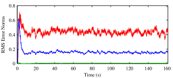
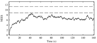
Figure 9: Performance of an UKF using a plain quaternion (top to bottom): Trajectory estimated, RMS error norms as in Fig. 5, NEES, from 50 Monte Carlo runs. The NEES is slightly too low (ca. by 1), probably because by using $\sigma_{\omega}^{2}$ as process noise covariance in all 4 quaternion components, the filter “thinks” there is process noise on the norm of the quaternion, while in fact there is none. The time-averaged error is $0.434\,m$, $1.71\times 10^{-2}\,rad$, and $0.160\,m/s$ in position, orientation, and velocity, respectively. This is slightly worse than for the $\mathbin{\text{\raisebox{-0.86108pt}{$\boxplus$}}}$-method, probably caused by the fact, that the quaternion is not fully normalized making the filter use the false DOF created by the quaternion’s norm to fit to the measurements.

6.2 Extension to Colored Noise Errors

GPS errors are correlated and hence a INS-GPS filter should model colored not white noise. Therefor, a bias vector must be added to the state:

⬇

...

((vect<3>, gps_bias))

)

The bias $b=$gps_bias follows the process model

$$b_{t+1}=\exp\left(-\tfrac{dt}{T}\right)b_{t}+\operatorname{\mathcal{N}}\!\left(0,\,\left(1\!-\!\exp\left(-\tfrac{2dt}{T}\right)\right)\sigma_{b}^{2}\operatorname{I}_{3}\right)$$

which realizes an autocorrelation with a given variance $\operatorname{\operatorname{Cov}}(b_{t})=\sigma_{b}^{2}\operatorname{I}_{3}$ and specified exponential decay $\operatorname{\operatorname{cor}}(b_{t},b_{t+k})=\exp\left(-\tfrac{k\cdot dt}{T}\right)$. The formula is taken from the textbook by Grewal [13, (8.76), (8.78)] and implemented in process_model by

and in process_noise_cov by

⬇

gps_cnoise*(1-exp(-2*dt/T_pos)));

The initial covariance is also set to $\sigma_{b}^{2}$:

Finally, gps_measurement_model adds the bias:

Figure 10 shows the performance of the modified filter with a simulation that includes colored noise on the GPS measurement ($\sigma_{b}^{2}=5\text{m}$, $T=1800\text{s}$).

This example shows that MTK and UKFoM allow for rapidly trying out different representations and models without being hindered by implementing bookkeeping issues. In a similar way, omitted here for lack of space, gyroscope and accelerometer bias can be integrated. Beyond that, further improvement would require operating on GPS pseudo-ranges (tightly coupled setup), with the state augmented by biases compensating for the various error sources (receiver clock error, per-satellite clock errors, ephemeris errors, atmospheric delays, etc.; [13, Ch. 5]).

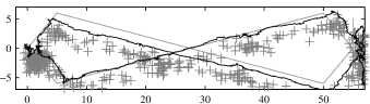
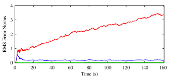
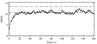
Figure 10: Performance of the $\mathbin{\text{\raisebox{-0.86108pt}{$\boxplus$}}}$-method UKF with colored noise (top to bottom): Trajectory estimated, error norms as in Fig. 5, NEES from 50 Monte Carlo runs. The filter is consistent, notably the position error grows over time. This is as expected: The filter knows its initial position and from this it can initially deduce the GPS-bias with about $1\text{m}$ precision. However, over time the bias drifts and with the inertial system being to imprecise, their is no information on the new bias and hence the position error grows. Velocity and orientation error keep low, because these are deduced from the relative position of GPS measurements where the bias cancels out.

6.3 Pose Relation Graph Optimization

To show the benefit of our $\mathbin{\text{\raisebox{-0.86108pt}{$\boxplus$}}}$-approach we optimized several 3D pose graphs using our manifold representation and compared it to the singular representations of Euler angles and matrix exponential (see Section 3.6.3), as well as a four dimensional quaternion representation. When using Gauss-Newton optimization the latter would fail, due to the rank-deficity of the problem, so we added the pseudo measurement $|q|=1$.

First, we show that the $\mathbin{\text{\raisebox{-0.86108pt}{$\boxplus$}}}$-method works on real-world data sets. Figure 11 shows a simple 2D landmark SLAM problem (DLR/Spatial Cognition data set [26]). Figure  12 shows the 3D Stanford multi-storey parking garage data set, where the initial estimate is so good, most methods work well.

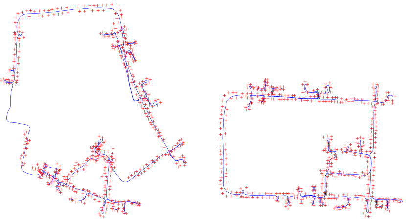
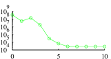
Figure 11: The DLR data set [26] before (left) and after (right) Gauss-Newton optimization. We also show the residual sum of squares over iteration steps (top, right). No comparison is made, as in 2D the $\mathbin{\text{\raisebox{-0.86108pt}{$\boxplus$}}}$-operator only encapsulates the handling of angular periodicity.

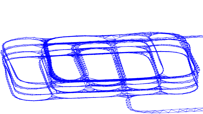
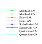
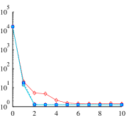
Figure 12: Residual sum of squares over iteration steps of Gauss-Newton (GN) and Levenberg-Marquardt (LM) optimization on the Stanford parking garage data set as used in [14]. Gauss-Newton with Euler-angles is clearly inferior to all other representations, however being far away from singularities, it still converges.

Second, for a quantitative comparison, we use the simulated dataset from [19, supplement], shown in Figure 13 and investigate how the different state representations behave under increasing noise levels. Figure 14 shows the results.

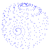
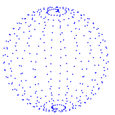
Figure 13: The sphere400 dataset [19] generated by a virtual robot driving on a 3D sphere. It consists of a set of 400 three-dimensional poses and about 780 noisy constraints between them. The constraints stem from motion between consecutive poses or relations to previously visited poses. Poses are initialized from motion constraints (left) and then optimized with our SLoM framework.

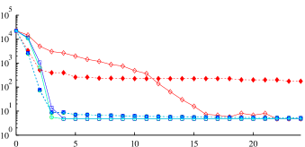
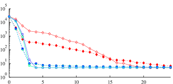
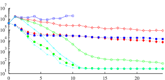
Figure 14: Residual sum of squares over iteration steps of Gauss-Newton and Levenberg-Marquardt with different state representations on the dataset in Fig. 13 (see Figure 12 for legend). The same data set was optimized using original noise (top) and with additional noises of 0.01 (middle) and 0.1 rad/m (bottom). For the latter two, the median of 31 runs is plotted. Plots ending unfinished indicate that more than half the optimizations could not be finished due to a singularity. The $\mathbin{\text{\raisebox{-0.86108pt}{$\boxplus$}}}$-method clearly out-performs the singular representations. For the high noise-level the quaternion representation is slightly better. However, when comparing run-times instead of iteration counts, the latter is slower due to the additional measurements and the larger state-space (7 DOF instead of 6 DOF per pose). Computation times were 63 ms for the 4D quaternion and 42 ms for the $\mathbin{\text{\raisebox{-0.86108pt}{$\boxplus$}}}$-approach per step. This fits well to the nominal factor of $(\tfrac{7}{6})^{3}\approx 1.59$ for the $O(n^{3})$-matrix decomposition. For Euler angle and matrix exponential, the evaluation took longer with times of 80 ms and 62 ms per step probably due to not hand-tuned code and the high number of trigonometric functions involved.

7 Conclusions

We have presented a principled way of providing a local vector-space view of a manifold $\mathcal{S}$ for use with sensor fusion algorithms. We have achieved this by means of an operator $\mathbin{\text{\raisebox{-0.86108pt}{$\boxplus$}}}:\mathcal{S}\times\mathbb{R}^{n}\to\mathcal{S}$ that adds a small vector-valued perturbation to a state in $\mathcal{S}$ and an inverse operator $\mathbin{\text{\raisebox{-0.86108pt}{$\boxminus$}}}:\mathcal{S}\times\mathcal{S}\to\mathbb{R}^{n}$ that computes the vector-valued perturbation turning one state into another. A space equipped with such operators is called a $\mathbin{\text{\raisebox{-0.86108pt}{$\boxplus$}}}$-manifold.

We have axiomatized this approach and lifted the concepts of Gaussian distribution, mean, and covariance to $\mathbin{\text{\raisebox{-0.86108pt}{$\boxplus$}}}$-manifolds therewith. The $\mathbin{\text{\raisebox{-0.86108pt}{$\boxplus$}}}$/$\mathbin{\text{\raisebox{-0.86108pt}{$\boxminus$}}}$ operators allow for the integration of manifolds into generic estimation algorithms such as least-squares or the UKF mainly by replacing $+$ and $-$ with $\mathbin{\text{\raisebox{-0.86108pt}{$\boxplus$}}}$ and $\mathbin{\text{\raisebox{-0.86108pt}{$\boxminus$}}}$. For the UKF additionally the computation of the mean and the covariance update are modified.

The $\mathbin{\text{\raisebox{-0.86108pt}{$\boxplus$}}}$-method is not only an abstract mathematical framework but also a software engineering toolkit for implementing estimation algorithms. In the form of our Manifold Toolkit (MTK) implementation (and its MATLAB variant MTKM), it automatically derives $\mathbin{\text{\raisebox{-0.86108pt}{$\boxplus$}}}$/$\mathbin{\text{\raisebox{-0.86108pt}{$\boxminus$}}}$ operators for compound manifolds and mediates between a flat-vector and a structured-components view.

8 Acknowledgements

This work has been partially supported by the German Research Foundation (DFG) under grant SFB/TR 8 Spatial Cognition, as well as by the German Federal Ministry of Education and Research (BMBF) under grant 01IS09044B and grant 01IW10002 (SHIP – Semantic Integration of Heterogeneous Processes).

Appendix

Appendix A Mathematical Analysis of $\mathbin{\text{\raisebox{-0.86108pt}{$\boxplus$}}}$-Manifolds

In Section 3 we have introduced the $\mathbin{\text{\raisebox{-0.86108pt}{$\boxplus$}}}$-method from a conceptual point of view, including the axiomatization of $\mathbin{\text{\raisebox{-0.86108pt}{$\boxplus$}}}$-manifolds and the generalization of the probabilistic notions of expected value, covariance, and Gaussian distribution from vector spaces to $\mathbin{\text{\raisebox{-0.86108pt}{$\boxplus$}}}$-manifolds. We will now underpin this discussion with mathematical proofs.

A.1 $\mathbin{\text{\raisebox{-0.86108pt}{$\boxplus$}}}$-Manifolds

First, we recall the textbook definition of manifolds (see, e.g., [28]). We simplify certain aspects not relevant within the context of our method; this does not affect formal correctness. In particular, we view a manifold $\mathcal{S}$ as embedded as a subset $\mathcal{S}\subset\mathbb{R}^{s}$ into Euclidean space $\mathbb{R}^{s}$ from the outset; this is without loss of generality by Whitney’s embedding theorem, and simplifies the presentation for our purposes.

Definition 2 (Manifold [28]).

A ($C^{k}$-, or smooth) manifold is a pair $(\mathcal{S},\mathcal{F})$ (usually denoted just $\mathcal{S}$) consisting of a connected set $\mathcal{S}\subset\mathbb{R}^{s}$ and an atlas $\mathcal{F}=(U_{\alpha},\varphi_{\alpha})_{\alpha\in A}$, i.e. a family of charts $(U_{\alpha},\varphi_{\alpha})$ consisting of an open subset $U_{\alpha}$ of $\mathcal{S}$ and a homeomorphism $\varphi_{\alpha}:U_{\alpha}\to V_{\alpha}$ of $U_{\alpha}$ to an open subset $V_{\alpha}\subset\mathbb{R}^{n}$. Here, $U_{\alpha}$ being open in $\mathcal{S}$ means that there is an open set $\tilde{U}_{\alpha}\subset\mathbb{R}^{s}$ such that $U_{\alpha}=\mathcal{S}\cap\tilde{U}_{\alpha}$. These data are subject to the following requirements.

1. The charts in $\mathcal{F}$ cover $\mathcal{S}$, i.e. $\mathcal{S}=\bigcup_{\alpha\in A}U_{\alpha}$.

2. If $U_{\alpha}\cap U_{\beta}\neq\emptyset$, the transition map

   $$\varphi_{\alpha}\circ\varphi_{\beta}^{-1}:\varphi_{\beta}(U_{\alpha}\cap U_{\beta})\to\varphi_{\alpha}(U_{\alpha}\cap U_{\beta})$$ (77)

   is a $C^{k}$-diffeomorphism.

The number $n$ is called the dimension or the number of degrees of freedom of $\mathcal{S}$.

We recall the generalization of the definition of smoothness, i.e. being $k$ times differentiable, to functions defined on arbitrary (not necessarily open) subsets $\mathcal{S}\subset\mathbb{R}^{s}$:

Definition 3 (Smooth Function).

For $\mathcal{S}\subset\mathbb{R}^{s}$, a function $f:\mathcal{S}\to\mathbb{R}^{n}$ is called smooth, i.e. $C^{k}$, in $x\in\mathcal{S}$ if there exists an open neighbourhood $U\subset\mathbb{R}^{s}$ of $x$ and a smooth function $\tilde{f}:U\to\mathbb{R}^{n}$ that extends $f|_{U\cap\mathcal{S}}$.

Next we show that every $\mathbin{\text{\raisebox{-0.86108pt}{$\boxplus$}}}$-manifold is indeed a manifold, justifying the name. The reverse is not true in general.

Lemma 1.

Every $\mathbin{\text{\raisebox{-0.86108pt}{$\boxplus$}}}$-manifold is a manifold, with the atlas $(U_{x},\varphi_{x})_{x\in\mathcal{S}}$ where

$$U_{x}=\left\{y\mid y\mathbin{\text{\raisebox{-0.86108pt}{$\boxminus$}}}x\in V\right\}$$ (78)

$$\varphi_{x}:U_{x}\to V,\;y\mapsto y\mathbin{\text{\raisebox{-0.86108pt}{$\boxminus$}}}x.$$ (79)

(This result will be sharpened later in Corollary 1.)

Proof.

$\mathcal{S}$ is connected, as $\gamma:\lambda\mapsto x\mathbin{\text{\raisebox{-0.86108pt}{$\boxplus$}}}(\lambda(y\mathbin{\text{\raisebox{-0.86108pt}{$\boxminus$}}}x))$ is a path from $\gamma(0)=x$ by (11a) to $\gamma(1)=y$ by (11b). From (11c) we have that $\varphi_{x}^{-1}(\delta)=x\mathbin{\text{\raisebox{-0.86108pt}{$\boxplus$}}}\delta$ is injective on $V$, and therefore bijective onto its image $U_{x}$. As both $\varphi_{x}$ and $\varphi_{x}^{-1}$ are required to be smooth, $\varphi_{x}$ is a diffeomorphism, in particular a homeomorphism. The set $U_{x}$ is open in $\mathcal{S}$, as it is the preimage of $V$ under the continuous function $\varphi_{x}$, and since $x\in U_{x}$ we have $\mathcal{S}=\bigcup_{x\in\mathcal{S}}U_{x}$. Finally, the transition map $\varphi_{x}\circ\varphi_{y}^{-1}$ is a composite of diffeomorphisms and therefore diffeomorphic. ∎

A.2 Induced Metric

Lemma 2.

The operation $\mathbin{\text{\raisebox{-0.86108pt}{$\boxminus$}}}$ defines a metric $\mathrm{d}$ on $\mathcal{S}$ by

$$\mathrm{d}_{\mathcal{S}}(x,y):=\left\|y\mathbin{\text{\raisebox{-0.86108pt}{$\boxminus$}}}_{\mathcal{S}}x\right\|.$$ (80)

Proof.

Positive definiteness of $\mathrm{d}$ follows from Axiom (11a) and positive definiteness of $\left\|\cdot\right\|$.

Symmetry can be shown using (11d):

$$\mathrm{d}(x,y) =\left\|y\mathbin{\text{\raisebox{-0.86108pt}{$\boxminus$}}}x\right\|=\left\|(y\mathbin{\text{\raisebox{-0.86108pt}{$\boxplus$}}}0)\mathbin{\text{\raisebox{-0.86108pt}{$\boxminus$}}}(y\mathbin{\text{\raisebox{-0.86108pt}{$\boxplus$}}}(x\mathbin{\text{\raisebox{-0.86108pt}{$\boxminus$}}}y))\right\|$$

$$\leq\left\|x\mathbin{\text{\raisebox{-0.86108pt}{$\boxminus$}}}y\right\|=\mathrm{d}(y,x)$$ (81)

and symmetrically, which implies equality. The triangle inequality also follows from (11d):

$$\mathrm{d}(x,z) =\left\|z\mathbin{\text{\raisebox{-0.86108pt}{$\boxminus$}}}x\right\|$$ (82)

$$=\left\|(y\mathbin{\text{\raisebox{-0.86108pt}{$\boxplus$}}}(z\mathbin{\text{\raisebox{-0.86108pt}{$\boxminus$}}}y))\mathbin{\text{\raisebox{-0.86108pt}{$\boxminus$}}}(y\mathbin{\text{\raisebox{-0.86108pt}{$\boxplus$}}}(x\mathbin{\text{\raisebox{-0.86108pt}{$\boxminus$}}}y))\right\|$$ (83)

$$\leq\left\|(z\mathbin{\text{\raisebox{-0.86108pt}{$\boxminus$}}}y)-(x\mathbin{\text{\raisebox{-0.86108pt}{$\boxminus$}}}y)\right\|$$ (84)

$$\leq\left\|(x\mathbin{\text{\raisebox{-0.86108pt}{$\boxminus$}}}y)\right\|+\left\|(z\mathbin{\text{\raisebox{-0.86108pt}{$\boxminus$}}}y)\right\|$$ (85)

$$=\mathrm{d}(x,y)+\mathrm{d}(y,z)\qed$$ (86)

A.3 Smooth Functions

Lemma 3.

For a map $f:\mathcal{S}\to\mathcal{M}$ between $\mathbin{\text{\raisebox{-0.86108pt}{$\boxplus$}}}$-manifolds $\mathcal{S}$ and $\mathcal{M}$, the following are equivalent for every $x\in\mathcal{S}$:

1. $f$ is smooth in $x$ (Definition 3)

2. $f(x\mathbin{\text{\raisebox{-0.86108pt}{$\boxplus$}}}_{\mathcal{S}}\delta)\mathbin{\text{\raisebox{-0.86108pt}{$\boxminus$}}}_{\mathcal{M}}z$ is smooth in $\delta$ at $\delta=0$ whenever $z\in\mathcal{M}$ is such that $f(x)\in U_{z}$.

Proof.

1 implies 2, as the concatenation of smooth functions is smooth.

For the converse implication, fix $z$ as in 2, let $\mathcal{S}\subset\mathbb{R}^{s}$ and $\mathcal{M}\subset\mathbb{R}^{m}$, and let $U\subset\mathbb{R}^{s}$ be a neighbourhood of $x$ such that $\mathbin{\text{\raisebox{-0.86108pt}{$\boxminus$}}}$ extends smoothly to $U\times\{x\}$. Then we extend $f$ smoothly to $\tilde{f}:U\to\mathbb{R}^{m}$ by

$$\tilde{f}(y) =z\mathbin{\text{\raisebox{-0.86108pt}{$\boxplus$}}}_{\mathcal{M}}(f(x\mathbin{\text{\raisebox{-0.86108pt}{$\boxplus$}}}_{\mathcal{S}}(y\mathbin{\text{\raisebox{-0.86108pt}{$\boxminus$}}}_{\mathcal{S}}x))\mathbin{\text{\raisebox{-0.86108pt}{$\boxminus$}}}_{\mathcal{M}}z).\qed$$ (87)

Replacing $\mathbin{\text{\raisebox{-0.86108pt}{$\boxplus$}}}$/$\mathbin{\text{\raisebox{-0.86108pt}{$\boxminus$}}}$ in $\delta\mapsto f(x\mathbin{\text{\raisebox{-0.86108pt}{$\boxplus$}}}\delta)\mathbin{\text{\raisebox{-0.86108pt}{$\boxminus$}}}z$ by the induced charts as in Lemma 1, we see that smoothness corresponds to the classical definition of smooth functions on manifolds [28, p. 32]:

$$f(x\mathbin{\text{\raisebox{-0.86108pt}{$\boxplus$}}}\delta)\mathbin{\text{\raisebox{-0.86108pt}{$\boxminus$}}}z=\varphi_{z}(f(\varphi_{x}^{-1}(\delta))),$$ (88)

with the right hand side required to be smooth in $\delta$ at $\delta=\varphi_{x}(x)=0$.

A direct consequence of this fact is

Corollary 1.

Every $\mathbin{\text{\raisebox{-0.86108pt}{$\boxplus$}}}$-manifold $\mathcal{S}\subset\mathbb{R}^{s}$ is an embedded submanifold of $\mathbb{R}^{s}$.

(Recall that this means that the embedding $\mathcal{S}\hookrightarrow\mathbb{R}^{s}$ is an immersion, i.e. a smooth map of manifolds that induces an injection of tangent spaces, and moreover that the topology of the manifold $\mathcal{S}$ is the subspace topology in $\mathbb{R}^{s}$ [28].)

Proof.

$\mathcal{S}$ carries the subspace topology by construction. Clearly, the injection $\mathcal{S}\hookrightarrow\mathbb{R}^{s}$ is smooth according to Definition 3, and hence as a map of manifolds by the above argument. Since tangent spaces are spaces of differential operators on smooth real-valued functions and moreover have a local nature [28], the immersion property amounts to every smooth real-valued function on an open subset of $\mathcal{S}$ extending to a smooth function on an open subset of $\mathbb{R}^{s}$, which is precisely the content of Definition 3. ∎

A.4 Isomorphic $\mathbin{\text{\raisebox{-0.86108pt}{$\boxplus$}}}$-Manifolds

For every type of structure, one has a notion of homomorphism, which describes mappings that preserve the relevant structure. The natural notion of morphism $\varphi:\mathcal{S}\to\mathcal{M}$ of $\mathbin{\text{\raisebox{-0.86108pt}{$\boxplus$}}}$-manifolds is a smooth map $\varphi:\mathcal{S}\to\mathcal{M}$ that is homomorphic w.r.t. the algebraic operations $\mathbin{\text{\raisebox{-0.86108pt}{$\boxplus$}}}$ and $\mathbin{\text{\raisebox{-0.86108pt}{$\boxminus$}}}$, i.e.

$$\varphi(x\mathbin{\text{\raisebox{-0.86108pt}{$\boxplus$}}}_{\mathcal{S}}\delta) =\varphi(x)\mathbin{\text{\raisebox{-0.86108pt}{$\boxplus$}}}_{\mathcal{M}}\delta$$ (89)

$$\varphi(x\mathbin{\text{\raisebox{-0.86108pt}{$\boxminus$}}}_{\mathcal{S}}y) =\varphi(x)\mathbin{\text{\raisebox{-0.86108pt}{$\boxminus$}}}_{\mathcal{M}}\varphi(y).$$ (90)

As usual, an isomorphism is a bijective homomorphism whose inverse is again a homomorphism. Compatibility of inverses of homomorphisms with algebraic operations as above is automatic, so that an isomorphism $\varphi:\mathcal{S}\to\mathcal{M}$ of $\mathbin{\text{\raisebox{-0.86108pt}{$\boxplus$}}}$-manifolds is just a diffeomorphism $\varphi:\mathcal{S}\to\mathcal{M}$ (i.e. an invertible smooth map with smooth inverse) that is homomorphic w.r.t. $\mathbin{\text{\raisebox{-0.86108pt}{$\boxplus$}}}$ and $\mathbin{\text{\raisebox{-0.86108pt}{$\boxminus$}}}$. If such a $\varphi$ exists, $\mathcal{S}$ and $\mathcal{M}$ are isomorphic. It is clear that isomorphic $\mathbin{\text{\raisebox{-0.86108pt}{$\boxplus$}}}$-manifolds are indistinguishable as such, i.e. differ only w.r.t. the representation of their elements. We will give examples of isomorphic $\mathbin{\text{\raisebox{-0.86108pt}{$\boxplus$}}}$-manifolds in Appendix B; e.g. orthonormal matrices and unit quaternions form isomorphic $\mathbin{\text{\raisebox{-0.86108pt}{$\boxplus$}}}$-manifolds.

A.5 Defining Symmetric $\mathbin{\text{\raisebox{-0.86108pt}{$\boxplus$}}}$-Manifolds

Most $\mathbin{\text{\raisebox{-0.86108pt}{$\boxplus$}}}$-manifolds arising in practice are manifolds with inherent symmetries. This can be exploited by defining $\mathbin{\text{\raisebox{-0.86108pt}{$\boxplus$}}}$ at one reference element and pulling this structure back to the other elements along the symmetry.

Formally, we describe the following procedure for turning an $n$-dimensional manifold $\mathcal{S}$ with sufficient symmetry into a $\mathbin{\text{\raisebox{-0.86108pt}{$\boxplus$}}}$-manifold. The first step is to define a smooth and surjective function $\psi:\mathbb{R}^{n}\to\mathcal{S}$ which is required to be locally diffeomorphic, i.e. for a neighborhood $V$ of $0\in\mathbb{R}^{n}$ it must have a smooth inverse $\varphi:=\psi^{-1}$. As $\psi$ is surjective, $\varphi$ can be extended globally to a (not necessarily smooth) function $\varphi:\mathcal{S}\to\mathbb{R}^{n}$ such that $\psi\circ\varphi=\operatorname{id}_{\mathcal{S}}$.

The next step is to define, for every $x\in\mathcal{S}$, a diffeomorphic transformation $R_{x}:\mathcal{S}\to\mathcal{S}$ (visually a “rotation”) such that $R_{x}(\psi(0))=x$. We can then define

$$x\mathbin{\text{\raisebox{-0.86108pt}{$\boxplus$}}}\delta :=R_{x}(\psi(\delta)), y\mathbin{\text{\raisebox{-0.86108pt}{$\boxminus$}}}x :=\varphi(R_{x}^{-1}(y)).$$ (91)

Since $x\mathbin{\text{\raisebox{-0.86108pt}{$\boxplus$}}}0=R_{x}(\psi(0))=x$, Axiom (11a) holds under this construction. Axiom (11b) holds as we require $\psi\circ\varphi=\operatorname{id}_{\mathcal{S}}$ globally. Finally, as $\varphi\circ\psi=\operatorname{id}_{V}$ Axiom (11c) is fulfilled for $\delta\in V$ as required. Axiom (11d) depends on $\psi$ and $R_{x}$ and needs to be established on a case-by-case basis.

A.6 Lie-Groups as $\mathbin{\text{\raisebox{-0.86108pt}{$\boxplus$}}}$-Manifolds

For connected Lie-groups [28, Chap. 20], i.e. manifolds with a diffeomorphic group structure, the above steps are very simple. On the one hand the mapping $\psi:\mathbb{R}^{n}\to\mathcal{S}$ can be defined using the exponential map [28, p. 522], which is a locally diffeomorphic map from a 0-neighborhood in the Lie-algebra (a vector space diffeomorphic to $\mathbb{R}^{n}$) to a neighborhood of the unit element in $\mathcal{S}$. For compact Lie-groups, the exponential map is also surjective, with global inverse $\log$.

The transformation $R_{x}$ can be simply defined as $R_{x}(y):=x\cdot y$ (or alternatively $R_{x}(y):=y\cdot x$) using the group’s multiplication:

$$x\mathbin{\text{\raisebox{-0.86108pt}{$\boxplus$}}}\delta :=x\cdot\exp(\delta), y\mathbin{\text{\raisebox{-0.86108pt}{$\boxminus$}}}x :=\log(x^{-1}\cdot y).$$ (92)

Again (11a)-(11c) follow from the construction in Appendix A.5. Axiom (11d) reduces to whether

$$\left\|(x\mathbin{\text{\raisebox{-0.86108pt}{$\boxplus$}}}\delta_{1})\mathbin{\text{\raisebox{-0.86108pt}{$\boxminus$}}}(x\mathbin{\text{\raisebox{-0.86108pt}{$\boxplus$}}}\delta_{2})\right\|$$ (93)

$$=\left\|\log\left(\left(x\cdot\exp\delta_{2}\right)^{-1}\cdot\left(x\cdot\exp\delta_{1}\right)\right)\right\|$$ (94)

$$=\left\|\log\left(\exp(-\delta_{2})\cdot\exp\delta_{1}\right)\right\|$$ (95)

$$\stackrel{{\scriptstyle?}}{{\leq}}\left\|\delta_{1}-\delta_{2}\right\|.$$ (96)

We do not know of a result that would establish this fact in general, and instead prove the inequality individually for each case.

A.7 Cartesian Product of Manifolds

Lemma 4.

The Cartesian product of two $\mathbin{\text{\raisebox{-0.86108pt}{$\boxplus$}}}$-manifolds $\mathcal{S}_{1}$ and $\mathcal{S}_{2}$ is a $\mathbin{\text{\raisebox{-0.86108pt}{$\boxplus$}}}$-manifold $\mathcal{S}=\mathcal{S}_{1}\times\mathcal{S}_{2}$, with $V=V_{1}\times V_{2}$ and

$$(x_{1},x_{2})\mathbin{\text{\raisebox{-0.86108pt}{$\boxplus$}}}\left[\begin{smallmatrix}\delta_{1}\\ \delta_{2}\end{smallmatrix}\right] =(x_{1}\mathbin{\text{\raisebox{-0.86108pt}{$\boxplus$}}}_{\mathcal{S}_{1}}\delta_{1},x_{2}\mathbin{\text{\raisebox{-0.86108pt}{$\boxplus$}}}_{\mathcal{S}_{2}}\delta_{2})$$ (97)

$$(y_{1},y_{2})\mathbin{\text{\raisebox{-0.86108pt}{$\boxminus$}}}(x_{1},x_{2}) =\left[\begin{smallmatrix}y_{1}\mathbin{\text{\raisebox{-0.60275pt}{$\boxminus$}}}_{\mathcal{S}_{1}}x_{1}\\ y_{2}\mathbin{\text{\raisebox{-0.60275pt}{$\boxminus$}}}_{\mathcal{S}_{2}}x_{2}\end{smallmatrix}\right]$$ (98)

for $(x_{1},x_{2}),(y_{1},y_{2})\in\mathcal{S}:=\mathcal{S}_{1}\times\mathcal{S}_{2}$ and $\left[\begin{smallmatrix}\delta_{1}\\ \delta_{2}\end{smallmatrix}\right]\in\mathbb{R}^{n_{1}}\times\mathbb{R}^{n_{2}}$.

Proof.

Smoothness of $\mathbin{\text{\raisebox{-0.86108pt}{$\boxplus$}}}$ and $\mathbin{\text{\raisebox{-0.86108pt}{$\boxminus$}}}$ as well as Axioms (11a), (11b) and (11c) hold componentwise. For Axiom (11d), we see that

$$\left\|(x\mathbin{\text{\raisebox{-0.86108pt}{$\boxplus$}}}\delta)\mathbin{\text{\raisebox{-0.86108pt}{$\boxminus$}}}(x\mathbin{\text{\raisebox{-0.86108pt}{$\boxplus$}}}\varepsilon)\right\|^{2} =\left\|(x_{1}\mathbin{\text{\raisebox{-0.86108pt}{$\boxplus$}}}\delta_{1})\mathbin{\text{\raisebox{-0.86108pt}{$\boxminus$}}}(x_{1}\mathbin{\text{\raisebox{-0.86108pt}{$\boxplus$}}}\varepsilon_{1})\right\|^{2}$$

$$\quad+\left\|(x_{2}\mathbin{\text{\raisebox{-0.86108pt}{$\boxplus$}}}\delta_{2})\mathbin{\text{\raisebox{-0.86108pt}{$\boxminus$}}}(x_{2}\mathbin{\text{\raisebox{-0.86108pt}{$\boxplus$}}}\varepsilon_{2})\right\|^{2}$$

$$\leq\left\|\delta_{1}-\varepsilon_{1}\right\|^{2}+\left\|\delta_{2}-\varepsilon_{2}\right\|^{2}$$

$$=\left\|\delta-\varepsilon\right\|^{2}.\qed$$

A.8 Expected Value on $\mathbin{\text{\raisebox{-0.86108pt}{$\boxplus$}}}$-Manifolds

Also using Axiom (11d), we prove that the definition of the expected value by a minimization problem in (15) implies the implicit definition (16):

Lemma 5.

For a random variable $X:\Omega\rightarrow\mathcal{S}$ and $\mu\in\mathcal{S}$,

$$\operatorname{\operatorname{E}}\left\|X\mathbin{\text{\raisebox{-0.86108pt}{$\boxminus$}}}\mu\right\|^{2}=\min_{\mu\in\mathcal{S}}!\Rightarrow\operatorname{\operatorname{E}}(X\mathbin{\text{\raisebox{-0.86108pt}{$\boxminus$}}}\mu)=0.$$ (99)

Proof.

Let $\mu:=\operatornamewithlimits{argmin}_{\mu}\operatorname{\operatorname{E}}\left\|X\mathbin{\text{\raisebox{-0.86108pt}{$\boxminus$}}}\mu\right\|^{2}$. Then

$$\operatorname{\operatorname{E}} \left\|X\mathbin{\text{\raisebox{-0.86108pt}{$\boxminus$}}}\mu\right\|^{2}\leq\operatorname{\operatorname{E}}\left\|X\mathbin{\text{\raisebox{-0.86108pt}{$\boxminus$}}}(\mu\mathbin{\text{\raisebox{-0.86108pt}{$\boxplus$}}}\operatorname{\operatorname{E}}(X\mathbin{\text{\raisebox{-0.86108pt}{$\boxminus$}}}\mu))\right\|^{2}$$ (100)

$$=\operatorname{\operatorname{E}}\left\|(\mu\mathbin{\text{\raisebox{-0.86108pt}{$\boxplus$}}}(X\mathbin{\text{\raisebox{-0.86108pt}{$\boxminus$}}}\mu))\mathbin{\text{\raisebox{-0.86108pt}{$\boxminus$}}}(\mu\mathbin{\text{\raisebox{-0.86108pt}{$\boxplus$}}}\operatorname{\operatorname{E}}(X\mathbin{\text{\raisebox{-0.86108pt}{$\boxminus$}}}\mu))\right\|^{2}$$ (101)

$$\leq\operatorname{\operatorname{E}}\left\|(X\mathbin{\text{\raisebox{-0.86108pt}{$\boxminus$}}}\mu)-\operatorname{\operatorname{E}}(X\mathbin{\text{\raisebox{-0.86108pt}{$\boxminus$}}}\mu)\right\|^{2}$$ (102)

$$=\operatorname{\operatorname{E}}\left\|X\mathbin{\text{\raisebox{-0.86108pt}{$\boxminus$}}}\mu\right\|^{2}-\left\|\operatorname{\operatorname{E}}(X\mathbin{\text{\raisebox{-0.86108pt}{$\boxminus$}}}\mu)\right\|^{2}$$ (103)

Hence, $\operatorname{\operatorname{E}}(X\mathbin{\text{\raisebox{-0.86108pt}{$\boxminus$}}}\mu)=0$. ∎

A.9 (Gaussian) Distributions on $\mathbin{\text{\raisebox{-0.86108pt}{$\boxplus$}}}$-Manifolds

The basic idea of (12) in Section 3.4 was to map a distribution $X:\Omega\to\mathbb{R}^{n}$ to a distribution $Y:\Omega\to\mathcal{S}$ by defining $Y:=\mu\mathbin{\text{\raisebox{-0.86108pt}{$\boxplus$}}}X$ for some $\mu\in\mathcal{S}$. The problem is that in general $\mathbin{\text{\raisebox{-0.86108pt}{$\boxplus$}}}$ is not injective. Thus (infinitely) many $X$ are mapped to the same $Y$, which makes even simple things such as computing $p(Y=y)$ for a given $y\in\mathcal{S}$ complicated, not to mention maximizing likelihoods.

A pragmatic approach is to “cut off” the distribution $X$ where $\mathbin{\text{\raisebox{-0.86108pt}{$\boxplus$}}}$ becomes ambiguous, i.e. define a distribution $\tilde{X}$ with

$$\operatorname{\operatorname{p}}(\tilde{X}=x):=\operatorname{\operatorname{p}}(X=x\mid X\in V)$$ (104)

This can be justified because, if $V$ is large compared to the covariance, $P(X\notin V)$ is small and the cut-off error is negligible. In practice, the fact that noise usually does not really obey a normal distribution leads to a much bigger error.

Now (12) simplifies to

$$\operatorname{\operatorname{p}}(\mu\mathbin{\text{\raisebox{-0.86108pt}{$\boxplus$}}}\tilde{X}=y)=\operatorname{\operatorname{p}}(\tilde{X}=y\mathbin{\text{\raisebox{-0.86108pt}{$\boxminus$}}}\mu),$$ (105)

because $\mathbin{\text{\raisebox{-0.86108pt}{$\boxplus$}}}$ is bijective for $\tilde{X}\in V$. We also find that for normal distributed noise, the maximum likelihood solution is the least squares solution.

Lemma 6.

For random variables $X:\Omega\rightarrow\mathcal{S}$, $Z:\Omega\rightarrow\mathcal{M}$, a measurement $z\in\mathcal{M}$, and a measurement function $f:\mathcal{S}\rightarrow\mathcal{M}$, with $f(X)=z\mathbin{\text{\raisebox{-0.86108pt}{$\boxplus$}}}\tilde{\varepsilon}$ and $\tilde{\varepsilon}\sim\operatorname{\mathcal{N}}\!\left(0,\,\Sigma\right)$ under the precondition $\tilde{\varepsilon}\in V$, the $x$ with largest likelihood $p(Z=z|X=x,\tilde{\varepsilon}\in V)$ is the one that minimizes $\frac{1}{2}\left\|f(x)\mathbin{\text{\raisebox{-0.86108pt}{$\boxminus$}}}{}z\right\|^{2}_{\Sigma}$.

Proof.

$$\operatorname{\operatorname{p}}(Z =z|X=x,\tilde{\varepsilon}\in V)=$$ (106)

$$\operatorname{\operatorname{p}}(z \mathbin{\text{\raisebox{-0.86108pt}{$\boxplus$}}}\tilde{\varepsilon}=f(x)|\tilde{\varepsilon}\in V)=\operatorname{\operatorname{p}}(\tilde{\varepsilon}=f(x)\mathbin{\text{\raisebox{-0.86108pt}{$\boxminus$}}}{}z)$$

$$\propto\exp\!\left(-\tfrac{1}{2}\left\|f(x)\mathbin{\text{\raisebox{-0.86108pt}{$\boxminus$}}}{}z\right\|^{2}_{\Sigma}\right)=\max!$$ (107)

$$\Leftrightarrow\;-\ln \left(\exp\!\left(-\tfrac{1}{2}\left\|f(x)\mathbin{\text{\raisebox{-0.86108pt}{$\boxminus$}}}{}z\right\|^{2}_{\Sigma}\right)\right)$$

$$=\frac{1}{2}\left\|f(x)\mathbin{\text{\raisebox{-0.86108pt}{$\boxminus$}}}{}z\right\|^{2}_{\Sigma}=\min!$$ (108)

Thus the classical approach of taking the negative log-likelihood shows the equivalence. ∎

Appendix B Examples of $\mathbin{\text{\raisebox{-0.86108pt}{$\boxplus$}}}$-Manifolds

In this appendix we will show Axioms (11) for the $\mathbin{\text{\raisebox{-0.86108pt}{$\boxplus$}}}$-manifolds discussed in Section 3.6 and further important examples. All, except $\mathbb{R}/2\pi\mathbb{Z}$ are based on either rotation matrices $SO(n)$ or unit vectors $S^{n}$, so we start with these general ones. Often several representations are possible, i.e. $\mathbb{R}/2\pi\mathbb{Z}$, $SO(2)$, or $S^{1}$ for 2D rotations and $SO(3)$ or $\mathbb{H}$ for 3D rotations. We will show these representations to be isomorphic, so in particular, Axiom (11d) holds for all if it holds for one.

B.1 The Rotation Group $SO(n)$

Rotations are length, handedness, and origin preserving transformations of $\mathbb{R}^{n}$. Formally they are defined as a matrix-group

$$SO(n)=\left\{Q\in\mathbb{R}^{n\times n}\mid Q^{\top}Q=\operatorname{I},\det Q=1\right\}.$$

Being subgroups of $Gl(n)$, the $SO(n)$ are Lie-groups. Thus we can use the construction in (92):

$$x\mathbin{\text{\raisebox{-0.86108pt}{$\boxplus$}}}{}\delta=x\exp\delta\quad y\mathbin{\text{\raisebox{-0.86108pt}{$\boxminus$}}}{}x=\log\left(x^{-1}y\right)$$ (109)

The matrix exponential is defined by the usual power series $\exp\delta=\sum_{i=0}^{\infty}\frac{1}{i!}\delta^{i}$, where the vector $\delta$ is converted to an antisymmetric matrix (we omit the $\hat{\phantom{\delta}}$ commonly indicating this). The logarithm is the inverse of $\exp$. The most relevant $SO(2)$, $SO(3)$ have analytic formulas, [34, 6] give general numerical algorithms.

(109) fulfills axioms (11a)–(11c) for suitable $V$ by the construction using the Lie-group structure. We conjecture that we can take $V=B_{\pi}(0)$, and that the remaining axiom (11d) also holds in general. We prove this for $n=2$ using an isomorphism to $\mathbb{R}/2\pi\mathbb{Z}$ (App. B.3) and for $n=3$ using an isomorphism to $\mathbb{H}$ (App. B.6).

B.2 Directions in $\mathbb{R}^{n+1}$ as Unit Vectors $S^{n}$

Another important manifold is the unit-sphere

$$S^{n}=\left\{x\in\mathbb{R}^{n+1}\mid\left\|x\right\|=1\right\},$$ (110)

the set of directions in $\mathbb{R}^{n+1}$. In general $S^{n}$ is no Lie-group, but we can still exploit symmetry by (91) (Sec. A.5) and define a mapping $R_{x}$ that takes the first unit vector $e_{1}$ to $x$. This is achieved by a Householder-reflection [35, Chap. 11.2].

$$R_{x}=\begin{cases}\left(\operatorname{I}-2\frac{vv^{\top}}{v^{\top}v}\right)X,\!&\text{for }v=x-e_{1}\neq 0,\\ \operatorname{I},&\text{for }x=e_{1}\!\end{cases}\!\!$$ (111)

Here $X$ is a matrix negating the second vector component. It makes $R_{x}$ the product of two reflections and hence a rotation. To define $e_{1}\mathbin{\text{\raisebox{-0.86108pt}{$\boxplus$}}}\delta$ we define $\exp$ and $\log$ for $S^{n}$ as

$$\exp\delta =\mathchoice{\left[\begin{matrix}\cos\left\|\delta\right\|\\ \operatorname{sinc}\left\|\delta\right\|\delta\end{matrix}\right]}{\bigl{[}\!\begin{smallmatrix}\cos\left\|\delta\right\|\\ \operatorname{sinc}\left\|\delta\right\|\delta\end{smallmatrix}\!\bigr{]}}{\bigl{[}\!\begin{smallmatrix}\cos\left\|\delta\right\|\\ \operatorname{sinc}\left\|\delta\right\|\delta\end{smallmatrix}\!\bigr{]}}{\bigl{[}\!\begin{smallmatrix}\cos\left\|\delta\right\|\\ \operatorname{sinc}\left\|\delta\right\|\delta\end{smallmatrix}\!\bigr{]}},$$ (112)

$$\log\mathchoice{\left[\begin{matrix}w\\ v\end{matrix}\right]}{\bigl{[}\!\begin{smallmatrix}w\\ v\end{smallmatrix}\!\bigr{]}}{\bigl{[}\!\begin{smallmatrix}w\\ v\end{smallmatrix}\!\bigr{]}}{\bigl{[}\!\begin{smallmatrix}w\\ v\end{smallmatrix}\!\bigr{]}} =\begin{cases}\operatorname{atan2}(0,w)e_{1}&v=0\\ \displaystyle\frac{\operatorname{atan2}(\left\|v\right\|,w)}{\left\|v\right\|}v&v\neq 0\end{cases}$$ (113)

We call these functions $\exp$ and $\log$, because they correspond to the usual power-series on complex numbers ($S^{1}$) and quaternions ($S^{3}$). In general, however, there is only a rough analogy.

Now, $S^{n}$ can be made a $\mathbin{\text{\raisebox{-0.86108pt}{$\boxplus$}}}$-manifold by (91), with $\psi=\exp$ and $\varphi=\psi^{-1}=\log$:

$$x\mathbin{\text{\raisebox{-0.86108pt}{$\boxplus$}}}{}\delta=R_{x}\exp\delta,\quad y\mathbin{\text{\raisebox{-0.86108pt}{$\boxminus$}}}{}x=\log(R_{x}^{\top}y)$$ (114)

The result looks the same as the corresponding definition (92) for Lie-groups, justifying the naming of (112) and (113) as $\exp$ and $\log$. We have that $\exp$ is left inverse to $\log$, and $\log$ is left inverse to $\exp$ on $\left\|\delta\right\|<\pi$. As proved in Lemma 7 (Appendix C), $\exp$ and $\log$ are smooth. Hence Axioms (11a), (11b), and (11c) hold for $V=B_{\pi}(0)$ (Sec.A.5). Axiom (11d) is proved as Lemma 11 in Appendix C.

The induced metric $\mathrm{d}(x,y)$ corresponds to the angle between $x$ and $y$ (Lemma 10).

Note that the popular stereographic projection cannot be extended to a $\mathbin{\text{\raisebox{-0.86108pt}{$\boxplus$}}}$-manifold, because it violates Axiom (11b).

Equipped with $\mathbin{\text{\raisebox{-0.86108pt}{$\boxplus$}}}$-manifolds for $SO(n)$ and $S^{n}$, we now discuss the most important special cases, first for $n=2$, then $n=3$.

B.3 2D Orientation as an Orthonormal Matrix

For planar rotations, $\exp$ in (109) takes an antisymmetric $2\times 2$ matrix, i.e. a number and returns the well-known 2D rotation matrix

$$x\mathbin{\text{\raisebox{-0.86108pt}{$\boxplus$}}}{}\delta =x\exp\delta,\quad y\mathbin{\text{\raisebox{-0.86108pt}{$\boxminus$}}}{}x=\log\left(x^{-1}y\right)$$ (115)

$$\exp\delta =\left[\begin{smallmatrix}\cos\delta&-\sin\delta\\ \sin\delta&\cos\delta\end{smallmatrix}\right],\log{}x=\operatorname{atan2}(x_{21},x_{11}).$$

The function $\exp$ is also an isomorphism between $\mathbb{R}/2\pi\mathbb{Z}$ (24) and $SO(2)$ (B.3), because the $2\pi$-periodicity of $\exp$ as a function matches the periodicity of $\mathbb{R}/2\pi\mathbb{Z}$ as a set of equivalence classes and $\exp{}x\cdot\exp\delta=\exp(x+\delta)$. The latter holds as multiplication in $SO(2)$ commutes. From this argument we see that $\mathbb{R}/2\pi\mathbb{Z}$ (Sec. 3.6.2) and $SO(2)$ are isomorphic $\mathbin{\text{\raisebox{-0.86108pt}{$\boxplus$}}}$-manifolds and also that axiom (11d) holds for the latter.

B.4 2D Orientation as a Complex Number

Using complex multiplication, $SO(2)$ is isomorphic to the complex numbers of unit-length, i.e. $S^{2}\subset\mathbb{C}$. For $n=2$, (112) and (113) simplify to

$$\exp_{S^{1}}\delta=\left[\begin{smallmatrix}\cos\delta\\ \sin\delta\end{smallmatrix}\right],\log_{S^{1}}\left[\begin{smallmatrix}x\\ y\end{smallmatrix}\right]=\operatorname{atan2}(y,x).$$ (116)

$R_{\left[\begin{smallmatrix}x\\ y\end{smallmatrix}\right]}$ equals complex multiplication with ${\left[\begin{smallmatrix}x\\ y\end{smallmatrix}\right]}$ or, as a matrix, $\left[\begin{smallmatrix}x&-y\\ y&x\end{smallmatrix}\right]$. This is because $R_{\left[\begin{smallmatrix}x\\ y\end{smallmatrix}\right]}$ it is a rotation mapping $e_{1}$ to $\left[\begin{smallmatrix}x\\ y\end{smallmatrix}\right]$ and there is only one such rotation on $S^{1}$. With these prerequisites, $S^{1}$ is isomorphic to $SO(2)$ by Lemma 14 as is $\mathbb{R}/2\pi\mathbb{Z}$.

B.5 Directions in 3D Space as $S^{2}$

The unit sphere is the most important example of a manifold that is not a Lie-group. This is a consequence of the “hairy ball theorem” [9], which states that on $S^{2}$ every continuous vector-field has a zero – if $S^{2}$ was a Lie-group, one could take the derivative of $x\cdot\delta$ for every $x$ and some fixed $\delta$ to obtain a vector field on $S^{2}$ without zeroes. With the same argument applied to $x\mathbin{\text{\raisebox{-0.86108pt}{$\boxplus$}}}\delta$, it is also impossible to give $S^{2}$ a $\mathbin{\text{\raisebox{-0.86108pt}{$\boxplus$}}}$-structure that is continuous in $x$. This is one reason why we did not demand continuity in $x$ for $\mathbin{\text{\raisebox{-0.86108pt}{$\boxplus$}}}$. It also shows that the discontinuity in (111) cannot be avoided in general (although it can for $S^{1}$ and $S^{3}$).

However, we can give a simpler analytical formula for $R_{x}$ in $S^{2}$:

$$\begin{split}R_{\left[\begin{smallmatrix}x\\ y\\ z\end{smallmatrix}\right]}:=\left[\begin{smallmatrix}x&-r&0\\ y&xc&-s\\ z&xs&c\\ \end{smallmatrix}\right],\alpha=\operatorname{atan2}(z,y),\\ c=\cos\alpha,s=\sin\alpha,r=\sqrt{x^{2}+z^{2}}\\ \end{split}$$ (117)

$$x\mathbin{\text{\raisebox{-0.86108pt}{$\boxplus$}}}{}\delta=R_{x}\exp\delta,\quad y\mathbin{\text{\raisebox{-0.86108pt}{$\boxminus$}}}{}x=\log(R_{x}^{\top}{}y)$$ (118)

The formula is discontinuous for $r=0$, but any value for $\alpha$ leads to a proper rotation matrix $R_{x}$. Therefore, neither $\mathbin{\text{\raisebox{-0.86108pt}{$\boxplus$}}}$ nor $\mathbin{\text{\raisebox{-0.86108pt}{$\boxminus$}}}$ are continuous in $x$, but they are smooth with respect to $\delta$ or $y$.

B.6 3D Orientation as a Unit Quaternion

The $\mathbin{\text{\raisebox{-0.86108pt}{$\boxplus$}}}$-manifold for quaternions $\mathbb{H}$ presented in Sec. 3.6.4, (29)-(31) is a special case of (112)-(114) for the unit sphere $S^{3}$. In the construction $R_{q}$ from (111) is conveniently replaced by $q^{-1}\cdot$, because $\mathbb{H}$ is a Lie-group. Also, $\exp$ and $\log$ correspond again to the usual functions for $\mathbb{H}$. The Axioms (11a)-(11c) are fulfilled for $V=B_{\pi}(0)$. Axiom (11d) is proved in Lemma 12.

The metric $\mathrm{d}(x,y)$ is the angle between $x$ and $y$, and also monotonically related to the simple Euclidean metric $\left\|x-y\right\|$ (Lemma 8).

Orthonormal matrices $SO(3)$ and unit quaternions $S^{3}/\{\pm 1\}$ are two different representations of rotations. Topologically this is called a universal covering [3, §12]. Hence, their $\mathbin{\text{\raisebox{-0.86108pt}{$\boxplus$}}}$-manifolds are isomorphic with the usual conversion operation

$$\begin{split}\varphi&\left[\begin{smallmatrix}w\\ x\\ y\\ z\end{smallmatrix}\right]=\left[\begin{smallmatrix}1-2(y^{2}+z^{2})&-2wz+2xy&-2wy+2xy\\ 2wz+2xy&1-2(x^{2}+z^{2})&-2wx+2yz\\ -2wy+2xz&2wx+2yz&1-2(x^{2}+y^{2})\end{smallmatrix}\right].\end{split}$$ (119)

For the proof we use that the well-known expressions $\exp_{SO(3)}(\alpha v/\left\|v\right\|)$ and $\exp_{S^{3}}(\tfrac{1}{2}\alpha v/\left\|v\right\|)$ for the rotation by an angle $\alpha$ around an axis $v$ in matrix and quaternion representation, with the exponentials defined in (26) and (30), so

$$\varphi (\exp_{S^{3}}(\delta/2))=\exp_{SO(3)}(\delta),$$ (120)

$$\varphi (q\mathbin{\text{\raisebox{-0.86108pt}{$\boxplus$}}}_{S^{3}}\delta)$$ (121)

$$=\varphi(q\exp_{S^{3}}(\delta/2))=\varphi(q)\varphi(\exp_{S^{3}}(\delta/2))$$ (122)

$$=\varphi(q)\exp_{SO(3)}(\delta)=\varphi(q)\mathbin{\text{\raisebox{-0.86108pt}{$\boxplus$}}}_{SO(3)}\delta.$$ (123)

The isomorphism also shows Axiom (11d) for $SO(3)$.

B.7 The Projective Space as $S^{n}$

Further important manifolds, e.g. in computer vision, are the projective spaces, informally non-Euclidean spaces where parallels intersect at infinity. Formally we define

$$\mathbb{P}^{n}:=\hbox{\raisebox{3.87495pt}{$(\mathbb{R}^{n+1}\setminus\left\{0\right\})$}{\raisebox{-0.43057pt}{\Large/}}\raisebox{-2.15277pt}{$(\mathbb{R}\setminus\left\{0\right\})$}}$$ (124)

and write

$$[x_{0}:x_{1}:\dots:x_{n}]=[x]=\left\{\lambda x\mid\lambda\in\mathbb{R}\setminus\left\{0\right\}\right\}$$ (125)

for the equivalence class modulo $\mathbb{R}\setminus\left\{0\right\}$ of a vector $x=(x_{1},\dots,x_{n})\in\mathbb{R}^{n+1}\setminus\left\{0\right\}$. In other words, $\mathbb{P}^{n}$ is the space of non-zero $(n+1)$-dimensional vectors modulo identification of scalar multiples.

As every point $[x]\in\mathbb{P}^{n}$ can uniquely be identified with the set $\bigl{\{}\tfrac{x}{\left\|x\right\|},\tfrac{-x}{\left\|x\right\|}\bigr{\}}\subset S^{n}$ we find that $\mathbb{P}^{n}\cong{S^{n}\!}/{\{\pm 1\}}$ and $S^{n}$ is a cover of $\mathbb{P}^{n}$. For $n=3$, we see the not quite intuitive fact that $\mathbb{P}^{3}\cong SO(3)$, so we can reuse the same $\mathbin{\text{\raisebox{-0.86108pt}{$\boxplus$}}}$-manifold there. For $\mathbb{P}^{2}$ we can basically reuse $S^{2}$ but care has to be taken due to the ambiguity of $x\equiv-x$. This can be solved by using $\operatorname{\overline{\log}}$ instead of $\log$ in $\mathbin{\text{\raisebox{-0.86108pt}{$\boxminus$}}}$, fulfilling Axioms (11) for $V=B_{\pi/2}$.

We cannot currently say anything about the induced metric on a projective space.

Appendix C Technical Proofs

Lemma 7.

The exponential $\exp\delta=\mathchoice{\left[\begin{matrix}\cos\left\|\delta\right\|\\ \operatorname{sinc}\left\|\delta\right\|\delta\end{matrix}\right]}{\bigl{[}\!\begin{smallmatrix}\cos\left\|\delta\right\|\\ \operatorname{sinc}\left\|\delta\right\|\delta\end{smallmatrix}\!\bigr{]}}{\bigl{[}\!\begin{smallmatrix}\cos\left\|\delta\right\|\\ \operatorname{sinc}\left\|\delta\right\|\delta\end{smallmatrix}\!\bigr{]}}{\bigl{[}\!\begin{smallmatrix}\cos\left\|\delta\right\|\\ \operatorname{sinc}\left\|\delta\right\|\delta\end{smallmatrix}\!\bigr{]}}$ from (112) is analytical on $\mathbb{R}^{n}$ and $\log$ is analytical on $S^{n}\setminus\left\{\mathchoice{\left[\begin{matrix}-1\\ \phantom{-}0\end{matrix}\right]}{\bigl{[}\!\begin{smallmatrix}-1\\ \phantom{-}0\end{smallmatrix}\!\bigr{]}}{\bigl{[}\!\begin{smallmatrix}-1\\ \phantom{-}0\end{smallmatrix}\!\bigr{]}}{\bigl{[}\!\begin{smallmatrix}-1\\ \phantom{-}0\end{smallmatrix}\!\bigr{]}}\right\}$. (Therefore, also $C^{\infty}$)

Proof.

The functions $\cos$ and $\operatorname{sinc}$ are both globally analytic, with Taylor series

$$\cos\left\|\delta\right\| =\sum_{k=0}^{\infty}\tfrac{(-1)^{k}\left\|\delta\right\|^{2k}}{(2k)!}=\sum_{k=0}^{\infty}\tfrac{(-\left\|\delta\right\|^{2})^{k}}{(2k)!},$$ (126)

$$\operatorname{sinc}\left\|\delta\right\| =\sum_{k=0}^{\infty}\tfrac{(-1)^{k}\left\|\delta\right\|^{2k}}{(2k+1)!}=\sum_{k=0}^{\infty}\tfrac{(-\left\|\delta\right\|^{2})^{k}}{(2k+1)!}.$$ (127)

Moreover, $\left\|\delta\right\|^{2}=\sum_{i=1}^{n}\delta_{i}^{2}$ is also analytic.

On the restriction $\exp:B_{\pi}\to S^{n}\setminus\left\{\mathchoice{\left[\begin{matrix}-1\\ \phantom{-}0\end{matrix}\right]}{\bigl{[}\!\begin{smallmatrix}-1\\ \phantom{-}0\end{smallmatrix}\!\bigr{]}}{\bigl{[}\!\begin{smallmatrix}-1\\ \phantom{-}0\end{smallmatrix}\!\bigr{]}}{\bigl{[}\!\begin{smallmatrix}-1\\ \phantom{-}0\end{smallmatrix}\!\bigr{]}}\right\}$ the inverse of $\exp$ is $\log$. In order to prove that $\log$ is analytic, we have to show that the Jacobian of $\exp$ has full rank. Using that the derivative of $\left\|\delta\right\|$ is $\delta^{\top}/\left\|\delta\right\|$ and hence the derivative of $\cos\left\|\delta\right\|$ is $\operatorname{sinc}\left\|\delta\right\|\delta^{\top}$, we show that for every $v\neq 0$:

$$\tfrac{\partial}{\partial\delta}(\exp\left\|\delta\right\|)v =\left[\begin{smallmatrix}\operatorname{sinc}\left\|\delta\right\|\delta^{\top}\\ \operatorname{sinc}\left\|\delta\right\|\operatorname{I}+\delta(\operatorname{sinc}^{\prime}\left\|\delta\right\|)/\left\|\delta\right\|\delta^{\top}\end{smallmatrix}\right]v$$ (128)

where the first component vanishes only for $\delta^{\top}v=0$ (as $\operatorname{sinc}x\neq 0$ for $\left|x\right|<\pi$). In this case the lower part becomes $\operatorname{sinc}\left\|\delta\right\|v$, which never vanishes for $\left\|\delta\right\|<\pi$. ∎

Lemma 8.

For two unit quaternions $a,b\in{}S^{3}$, there is a monotonic mapping between their Euclidean distance and the distance induced by $\mathbin{\text{\raisebox{-0.86108pt}{$\boxminus$}}}$:

$$\left\|a-b\right\|^{2}=f(\left\|a\mathbin{\text{\raisebox{-0.86108pt}{$\boxminus$}}}{}b\right\|),\text{with }f(\alpha)=2-2\cos(\alpha/2)$$ (129)

This also holds when antipodes are identified and both metrics are defined as the minimum obtained for any choice of representatives from the equivalence classes $\{a,-a\},\{b,-b\}$.

Proof.

We put $\delta:=b\mathbin{\text{\raisebox{-0.86108pt}{$\boxminus$}}}{}a=2\log(b^{-1}a)$. Then

$$\hskip-10.00002pt\left\|b-a\right\|^{2}=\left\|\bigl{[}\!\begin{smallmatrix}1\\ 0\end{smallmatrix}\!\bigr{]}-b^{-1}a\right\|^{2}$$ (130)

$$=\left\|\bigl{[}\!\begin{smallmatrix}1\\ 0\end{smallmatrix}\!\bigr{]}-\exp(\tfrac{1}{2}\delta)\right\|^{2}$$ (131)

$$=\left\|\left[\begin{smallmatrix}1-\cos(\tfrac{1}{2}\left\|\delta\right\|)\\ \operatorname{sinc}(\tfrac{1}{2}\left\|\delta\right\|)\tfrac{1}{2}\delta\end{smallmatrix}\right]\right\|^{2}$$ (132)

$$=(1-\cos(\tfrac{1}{2}\left\|\delta\right\|))^{2}+(\operatorname{sinc}(\tfrac{1}{2}\left\|\delta\right\|)\;(\tfrac{1}{2}\left\|\delta\right\|))^{2}$$

$$=(1-\cos(\tfrac{1}{2}\left\|\delta\right\|))^{2}+\sin^{2}(\tfrac{1}{2}\left\|\delta\right\|)$$ (133)

$$=2-2\cos(\tfrac{1}{2}\left\|\delta\right\|)$$ (134)

The inequality holds for every pair of antipodes $(a,b),(-a,b),(a,-b),(-a,-b)$ hence also for their minimum, which is by definition the distance of the equivalence classes. ∎

Lemma 9.

For two orthonormal matrices $A,B\in SO(3)$, there is a monotonic mapping between their Frobenius distance and the distance induced by $\mathbin{\text{\raisebox{-0.86108pt}{$\boxminus$}}}$:

$$\left\|B-A\right\|_{\mathrm{F}}^{2}=f(\left\|A\mathbin{\text{\raisebox{-0.86108pt}{$\boxminus$}}}{}B\right\|)\text{ with }f(\alpha)=4-4\cos\alpha.$$ (135)

Proof.

We put $\delta=A\mathbin{\text{\raisebox{-0.86108pt}{$\boxminus$}}}{}B$. Then

$$\left\|B-A\right\|_{\mathrm{F}}^{2} =\left\|A\mathbin{\text{\raisebox{-0.86108pt}{$\boxplus$}}}\delta-A\right\|_{\mathrm{F}}^{2}$$ (136)

$$=\left\|A\exp\delta-A\right\|_{\mathrm{F}}^{2}$$ (137)

$$=\left\|\exp\delta-\operatorname{I}\right\|_{\mathrm{F}}^{2}.$$ (138)

Let $$Q \delta x Q\delta=(\left\|\delta\right\|,0,0)^{\top} \exp(Q\delta)Q=Q\exp\delta$$ be an orthonormal matrix that rotates into -direction, i.e. . As , we have

$$=\left\|Q^{\top}\exp(Q\delta)Q-\operatorname{I}\right\|_{\mathrm{F}}^{2}$$ (139)

$$=\left\|\exp(Q\delta){}-\operatorname{I}\right\|_{\mathrm{F}}^{2}$$ (140)

$$=\left\|\exp(\left\|\delta\right\|,0,0)^{\top}-\operatorname{I}\right\|_{\mathrm{F}}^{2}$$ (141)

$$=\left\|\left[\begin{smallmatrix}0&0&0\\ 0&\cos\left\|\delta\right\|-1&-\sin\left\|\delta\right\|\\ 0&\sin\left\|\delta\right\|&\cos\left\|\delta\right\|-1\end{smallmatrix}\right]\right\|_{\mathrm{F}}^{2}$$ (142)

$$=2(\cos\left\|\delta\right\|-1)^{2}+2\sin^{2}\left\|\delta\right\|$$ (143)

$$=4-4\cos\left\|\delta\right\|.\qed$$ (144)

Lemma 10.

The curve $x\mathbin{\text{\raisebox{-0.86108pt}{$\boxplus$}}}(\lambda\delta)$, with $\lambda\in[0,1]$ and $\mathbin{\text{\raisebox{-0.86108pt}{$\boxplus$}}}$ defined by (114), is a geodetic on $S^{n}$ with arc-length $\left\|\delta\right\|$.

Proof.

We have

$$x \mathbin{\text{\raisebox{-0.86108pt}{$\boxplus$}}}(\lambda\delta)=R_{x}\exp(\lambda\delta)=R_{x}\bigl{[}\!\begin{smallmatrix}\cos(\lambda\left\|\delta\right\|)\\ \operatorname{sinc}(\lambda\left\|\delta\right\|)(\lambda\delta)\end{smallmatrix}\!\bigr{]}$$

$$=R_{x}\bigl{[}\!\begin{smallmatrix}\cos(\lambda\left\|\delta\right\|)\\ \sin(\lambda\left\|\delta\right\|)\delta/\left\|\delta\right\|\end{smallmatrix}\!\bigr{]}=R_{x}\left[\begin{smallmatrix}1&0\\ 0&\delta/\left\|\delta\right\|\end{smallmatrix}\right]\left[\begin{smallmatrix}\cos(\lambda\left\|\delta\right\|)\\ \sin(\lambda\left\|\delta\right\|)\end{smallmatrix}\right].$$

It can be seen that $x\mathbin{\text{\raisebox{-0.86108pt}{$\boxplus$}}}(\lambda\delta)$ is a circle segment with radius $1$ and hence a geodetic of length $\left\|\delta\right\|$ on $S^{n}$. ∎

Lemma 11.

For the $\mathbin{\text{\raisebox{-0.86108pt}{$\boxplus$}}}$ and $\mathbin{\text{\raisebox{-0.86108pt}{$\boxminus$}}}$ operators on the hypersphere $S^{n}$ defined in (114), Axiom (11d) holds (Fig. 15).

Proof.

By Lemma 10, the expression $\left\|(x\mathbin{\text{\raisebox{-0.86108pt}{$\boxplus$}}}\delta_{1})\mathbin{\text{\raisebox{-0.86108pt}{$\boxminus$}}}{}(x\mathbin{\text{\raisebox{-0.86108pt}{$\boxplus$}}}\delta_{2})\right\|$ involves a triangle of three geodetics $(x,x\mathbin{\text{\raisebox{-0.86108pt}{$\boxplus$}}}\delta_{1})$, $(x,x\mathbin{\text{\raisebox{-0.86108pt}{$\boxplus$}}}\delta_{2})$, and $(x\mathbin{\text{\raisebox{-0.86108pt}{$\boxplus$}}}\delta_{1},x\mathbin{\text{\raisebox{-0.86108pt}{$\boxplus$}}}\delta_{2})$. By the same lemma, the first two have length $\alpha=\left\|\delta_{1}\right\|$ and $\beta=\left\|\delta_{2}\right\|$. Hence by the spherical law of cosines, with $\gamma=\angle(\delta_{1},\delta_{2})$, the third has a length of

$$\hskip-10.00002pt\left\|(x\mathbin{\text{\raisebox{-0.86108pt}{$\boxplus$}}}\delta_{1})\mathbin{\text{\raisebox{-0.86108pt}{$\boxminus$}}}{}(x\mathbin{\text{\raisebox{-0.86108pt}{$\boxplus$}}}\delta_{2})\right\|$$ (145)

$$=\operatorname{acos}\left(\cos\alpha\cos\beta+\sin\alpha\sin\beta\cos\gamma\right)$$ (146)

$$\hskip-12.17223pt\mathrel{\hbox{$\displaystyle\mathop{\leq}\limits^{\text{Lemma \ref{lem:triangle}}}$}}\sqrt{\alpha^{2}+\beta^{2}-2\alpha\beta\cos\gamma}=\left\|\delta_{1}-\delta_{2}\right\|\qed$$ (147)

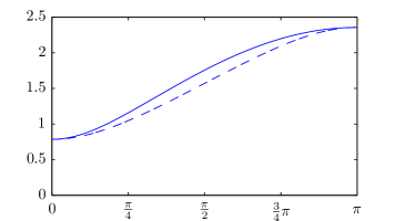
Figure 15: Spherical distance $\left\|(x\mathbin{\text{\raisebox{-0.86108pt}{$\boxplus$}}}\delta_{1})\mathbin{\text{\raisebox{-0.86108pt}{$\boxminus$}}}{}(x\mathbin{\text{\raisebox{-0.86108pt}{$\boxplus$}}}\delta_{2})\right\|$ (dashed) and Euclidean distance in the tangential plane $\left\|\delta_{1}-\delta_{2}\right\|$ (solid) plotted over the angle $\gamma$ between $\delta_{1}$ and $\delta_{2}$ for the case $\left\|\delta_{1}\right\|=\alpha=\frac{\pi}{4}$ and $\left\|\delta_{2}\right\|=\beta=\frac{\pi}{2}$. Confer both sides of (153) for the concrete terms plotted.

Lemma 12.

For the quaternion $\mathbin{\text{\raisebox{-0.86108pt}{$\boxplus$}}}$ and $\mathbin{\text{\raisebox{-0.86108pt}{$\boxminus$}}}$ operators defined in (29), Axiom (11d) holds (Fig. 15).

Proof.

We apply the definitions and notice from (31) that $\left\|\operatorname{\overline{\log}}{}q\right\|=\operatorname{acos}\left|\Re{}q\right|\leq\operatorname{acos}(\Re{}q)$ exploiting that $\left\|q\right\|=1$. Thus

$$\hskip-6.99997pt\left\|(x\mathbin{\text{\raisebox{-0.86108pt}{$\boxplus$}}}\delta_{1})\mathbin{\text{\raisebox{-0.86108pt}{$\boxminus$}}}{}(x\mathbin{\text{\raisebox{-0.86108pt}{$\boxplus$}}}\delta_{2})\right\|$$

$$=\left\|2\operatorname{\overline{\log}}\left((x\exp\tfrac{\delta_{1}}{2})^{-1}\cdot(x\exp\tfrac{\delta_{2}}{2})\right)\right\|$$ (148)

$$\leq 2\operatorname{acos}\Re\left(\exp\tfrac{-\delta_{1}}{2}\cdot\exp\tfrac{\delta_{2}}{2}\right)$$ (149)

$$=2\operatorname{acos}\Re\left(\bigl{[}\!\begin{smallmatrix}\cos(\left\|\delta_{1}\right\|/2)\\ -\operatorname{sinc}(\left\|\delta_{1}\right\|/2)/2\;\delta_{1}\end{smallmatrix}\!\bigr{]}\cdot\bigl{[}\!\begin{smallmatrix}\cos(\left\|\delta_{2}\right\|/2)\\ \operatorname{sinc}(\left\|\delta_{2}\right\|/2)/2\;\delta_{2}\end{smallmatrix}\!\bigr{]}\right).$$

Now we apply the definition of quaternion multiplication $\bigl{[}\!\begin{smallmatrix}r_{1}\\ v_{1}\end{smallmatrix}\!\bigr{]}\cdot\bigl{[}\!\begin{smallmatrix}r_{2}\\ v_{2}\end{smallmatrix}\!\bigr{]}=\bigl{[}\!\begin{smallmatrix}r_{1}r_{2}-v_{1}^{\top}v_{2}\\ \bullet\end{smallmatrix}\!\bigr{]}$ and substitute $\alpha=\left\|\delta_{1}\right\|/2$, $\beta=\left\|\delta_{2}\right\|/2$, and $\gamma=\angle(\delta_{1},\delta_{2})$. The term $v_{1}^{\top}v_{2}$ becomes $-\sin\alpha\sin\beta\cos\gamma$, and hence we can continue the above chain of equalities with

$$=2\operatorname{acos}\left(\cos\alpha\cos\beta+\sin\alpha\sin\beta\cos\gamma\right)$$ (150)

$$\hskip-12.17223pt\mathrel{\hbox{$\displaystyle\mathop{\leq}\limits^{\text{Lemma \ref{lem:triangle}}}$}}2\sqrt{\alpha^{2}+\beta^{2}-2\alpha\beta\cos\gamma}$$ (151)

$$=\left\|\delta_{1}-\delta_{2}\right\|.\qed$$ (152)

Lemma 13.

The distance on a sphere is less or equal to the Euclidean distance in the tangential plane (Fig. 15). Formally, for all $\alpha,\beta\geq 0,\gamma\in\mathbb{R}$

$$\begin{split}\operatorname{acos}\bigl{(}\cos\alpha\cos\beta+\sin\alpha\sin\beta\cos\gamma\bigr{)}\\ \quad\leq\sqrt{\alpha^{2}+\beta^{2}-2\alpha\beta\cos\gamma}.\end{split}$$ (153)

Proof.

If the right-hand side exceeds $\pi$, the inequality is trivial. Otherwise we substitute $\lambda:=\cos\gamma$ and take the cosine:

$$\begin{split}\cos\alpha\cos\beta+\sin\alpha\sin\beta\lambda\\ \quad\geq\cos\sqrt{\alpha^{2}+\beta^{2}-2\alpha\beta\lambda}.\end{split}$$ (154)

The proof idea is that the left-hand side of (154) is linear in $\lambda$, the right-hand side is convex in $\lambda$, and both are equal for $\lambda=\pm 1$. Formally, from the cosine addition formula we get

$$\cos\alpha\cos\beta-\sin\alpha\sin\beta =\cos(\alpha+\beta)$$ (155)

$$=\cos\sqrt{\alpha^{2}+\beta^{2}+2\alpha\beta},$$ (156)

$$\cos\alpha\cos\beta+\sin\alpha\sin\beta =\cos(\alpha-\beta)$$ (157)

$$=\cos\sqrt{\alpha^{2}+\beta^{2}-2\alpha\beta}.$$ (158)

Taking a $\frac{1-\lambda}{2}:\frac{1+\lambda}{2}$ convex combination of (155) and (157) we get the left-hand side of (154):

$$\cos\alpha\cos\beta+\sin\alpha\sin\beta\lambda$$ (159)

$$=\cos\alpha\cos\beta+\sin\alpha\sin\beta\left(\tfrac{1-\lambda}{2}(-1)+\tfrac{1+\lambda}{2}(+1)\right)$$

$$\begin{split}&=\phantom{+}\tfrac{1-\lambda}{2}\cos\sqrt{\alpha^{2}+\beta^{2}-2\alpha\beta}\\ &\phantom{=}+\tfrac{1+\lambda}{2}\cos\sqrt{\alpha^{2}+\beta^{2}+2\alpha\beta}\end{split}$$

$$\geq\cos\sqrt{\alpha^{2}+\beta^{2}+2\alpha\beta\left(\tfrac{1-\lambda}{2}(-1)+\tfrac{1+\lambda}{2}(+1)\right)}$$

$$=\cos\sqrt{\alpha^{2}+\beta^{2}+2\alpha\beta\lambda}.$$ (160)

The inequality comes from the convexity of the right-hand side of (154) in $\lambda$. We prove this by calculating its derivative

$$-\sin\sqrt{\alpha^{2}+\beta^{2}+2\alpha\beta\lambda}\;\frac{1}{2\sqrt{\alpha^{2}+\beta^{2}+2\alpha\beta\lambda}}\;2\alpha\beta$$

$$=-\operatorname{sinc}\sqrt{\alpha^{2}+\beta^{2}+2\alpha\beta\lambda}\;\alpha\beta$$ (161)

and observing that (161) increases monotonically until the square root exceeds $\pi$. ∎

Lemma 14.

The following function $\varphi$ is an $\mathbin{\text{\raisebox{-0.86108pt}{$\boxplus$}}}$-isomorphism between $S^{1}$ and $SO(2)$:

$$\varphi:S^{1}\rightarrow SO(2),\quad\varphi\left[\begin{smallmatrix}x\\ y\end{smallmatrix}\right]=\left[\begin{smallmatrix}x&-y\\ y&x\end{smallmatrix}\right].$$ (162)

Proof.

The map is bijective, because all matrices in $SO(2)$ are of the form (B.3). It also commutes with $\mathbin{\text{\raisebox{-0.86108pt}{$\boxplus$}}}$, since

$$\varphi(\left[\begin{smallmatrix}x\\ y\end{smallmatrix}\right]\mathbin{\text{\raisebox{-0.86108pt}{$\boxplus$}}}_{S^{1}}\delta) =\varphi(R_{\left[\begin{smallmatrix}x\\ y\end{smallmatrix}\right]}^{\top}\exp\delta)$$ (163)

$$=\varphi\left(\left[\begin{smallmatrix}x&-y\\ y&x\end{smallmatrix}\right]\left[\begin{smallmatrix}\cos\delta\\ \sin\delta\end{smallmatrix}\right]\right)$$ (164)

$$=\varphi\left(\left[\begin{smallmatrix}x\cos\delta-y\sin\delta\\ y\cos\delta+x\sin\delta\end{smallmatrix}\right]\right)$$ (165)

$$=\left[\begin{smallmatrix}x\cos\delta-y\sin\delta&-y\cos\delta-x\sin\delta\\ y\cos\delta+x\sin\delta&x\cos\delta-y\sin\delta\end{smallmatrix}\right]$$ (166)

$$=\left[\begin{smallmatrix}x&-y\\ y&x\end{smallmatrix}\right]\left[\begin{smallmatrix}\cos\delta&-\sin\delta\\ \sin\delta&\cos\delta\end{smallmatrix}\right]$$ (167)

$$=\left[\begin{smallmatrix}x&-y\\ y&x\end{smallmatrix}\right]\exp{\delta}$$ (168)

$$=\varphi\left(\left[\begin{smallmatrix}x\\ y\end{smallmatrix}\right]\right)\mathbin{\text{\raisebox{-0.86108pt}{$\boxplus$}}}_{SO^{2}}\delta.\qed$$ (169)

Appendix D Comparison to SPMap

In an SPMap [7] (originally 2D but extended to 3D) every geometric entity is represented by a reference pose ($SE(3)$) in an arbitrary, potentially overparametrized representation, and a perturbation vector parametrizing the entity relative to its reference pose in minimal parametrization. The estimation algorithm operates solely on the perturbation vector. This corresponds to $s\mathbin{\text{\raisebox{-0.86108pt}{$\boxplus$}}}\delta$, with $s$ being the reference pose and $\delta$ the perturbation vector. Actually, this concept and the idea that in most algorithms $\mathbin{\text{\raisebox{-0.86108pt}{$\boxplus$}}}$ can simply replace $+$ motivated the axiomatization of $\mathbin{\text{\raisebox{-0.86108pt}{$\boxplus$}}}$-systems we propose. Our contribution is to give this idea, which has been around for a while, a thorough mathematical framework more general than geometric entities.

If a geometric entity is “less than a pose”, e.g. a point, SPMap still uses a reference pose but the redundant DOFs, e.g. rotation, are removed from the perturbation vector. In our axiomatization the pose would simply be an overparametrization of a point. Using the notation of [7]

$$s\mathbin{\text{\raisebox{-0.86108pt}{$\boxplus$}}}\delta=s\oplus(B^{\top}\delta),$$ (170)

where $B$ is the so-called binding matrix that maps entries of $\delta$ to the DOF of a pose, and $\oplus$ is the concatenation of poses.

Analogously, the SPMap represents, e.g. a line as the pose’s $x$-axis with $x$-rotation and translation being redundant DOFs removed from the perturbation vector. Here lies a theoretical difference. Consider two such poses differing by an $x$-rotation. They represent the same line but differ in the effect of the perturbation vector, as $y$- and $z$-axes point into different directions. For us, the $\mathbin{\text{\raisebox{-0.86108pt}{$\boxplus$}}}$-system $\mathcal{S}$ would be a space of equivalence classes of poses. However, $\mathbin{\text{\raisebox{-0.86108pt}{$\boxplus$}}}$ maps from $\mathcal{S}\times\mathbb{R}^{n}$ to $\mathcal{S}$, so $s\mathbin{\text{\raisebox{-0.86108pt}{$\boxplus$}}}\delta$ must formally be the equivalent for equivalent poses $s$. The SPMap representation has the advantage that it is continuous both in the pose and the perturbation vector, which is not possible with our axiomatization due to the hairy ball theorem as discussed in Sec. B.5.

Overall, our contribution is the axiomatized and more general view, not limited to quotients of $SE(3)$ as with the SPMap. We currently investigate axiomatization of SPMap’s idea to allow different representatives of the same equivalence class to define different $\mathbin{\text{\raisebox{-0.86108pt}{$\boxplus$}}}$-co-ordinate systems. We avoided this here, because it adds another level of conceptual complexity.

References

- Abbeel [2008] P. Abbeel, Apprenticeship Learning and Reinforcement Learning with Application to Robotic Control, Ph.D. thesis, Department of Computer Science. Stanford University, 2008.
- Abrahams and Gurtovoy [2005] D. Abrahams, A. Gurtovoy, C++ Template Metaprogramming, Pearson Education, 2005.
- Altmann [1986] S.L. Altmann, Rotations, Quaternions and Double Groups, Oxford University Press, 1986.
- Bar-Shalom et al. [2001] Y. Bar-Shalom, X. Li, T. Kirubarajan, Estimation with Applications to Tracking and Navigation, John Wiley & Sons, Inc., 2001.
- Birbach [2008] O. Birbach, Accuracy Analysis of Camera-Inertial Sensor Based Ball-Trajectory Prediction, Master’s thesis, Universität Bremen, 2008.
- Cardosoa and Leitec [2010] J. Cardosoa, F. Leitec, Exponentials of skew-symmetric matrices and logarithms of orthogonal matrices, Journal of Computational and Applied Mathematics 233 (2010) 2867–2875.
- Castellanos et al. [1999] J.A. Castellanos, J. Montiel, J. Neira, J.D. Tards, The SPmap: A probablistic framework for simultaneous localization and map building, IEEE Transactions on Robotics and Automation 15 (1999) 948 – 952.
- Davison [2003] A. Davison, Real-time simultaneous localisation and mapping with a single camera, in: Proceedings of the International Conference on Computer Vision, 2003.
- Eisenberg and Guy [1979] M. Eisenberg, R. Guy, A proof of the hairy ball theorem, The American Mathematical Monthly 86 (1979) 571–574.
- Fisher [1953] R. Fisher, Dispersion on a sphere, Proceedings of the Royal Society of London. Series A, Mathematical and Physical Sciences 217 (1953) 295–305.
- Frese and Schröder [2006] U. Frese, L. Schröder, Theorie der Sensorfusion 2006, 2006. Universität Bremen, lecture notes #03-05-H-699.55.
- Gauss [1821] C.F. Gauss, Theoria combinationis observationum erroribus minimis obnoxiae, Commentationes societatis regiae scientiarum Gottingensis recentiores 5 (1821) 6–93.
- Grewal et al. [2007] M.S. Grewal, L.R. Weill, A.P. Andrews, Global Positioning Systems, Inertial Navigation, and Integration, John Wiley, 2nd edition, 2007.
- Grisetti et al. [2009] G. Grisetti, C. Stachniss, W. Burgard, Nonlinear Constraint Network Optimization for Efficient Map Learning, IEEE Transactions on Intelligent Transportation Systems 10 (2009) 428–439.
- Guennebaud et al. [2010] G. Guennebaud, B. Jacob, et al., Eigen 2.0.15, eigen.tuxfamily.org, 2010.
- Hertzberg [2008] C. Hertzberg, A Framework for Sparse, Non-Linear Least Squares Problems on Manifolds, Master’s thesis, Universität Bremen, 2008.
- Julier and Uhlmann [1996] S.J. Julier, J.K. Uhlmann, A General Method for Approximating Nonlinear Transformations of Probability Distributions, Technical Report, University of Oxford, 1996.
- Julier and Uhlmann [1997] S.J. Julier, J.K. Uhlmann, A new extension of the Kalman filter to nonlinear systems, in: Int. Symp. Aerospace/Defense Sensing, Simul. and Controls, Orlando, FL, 1997, pp. 182–193.
- Kaess et al. [2008] M. Kaess, A. Ranganathan, F. Dellaert, iSAM: Incremental smoothing and mapping, IEEE Transactions on Robotics 24 (2008) 1365–1378. openslam.org/iSAM.
- Kalman [1960] R.E. Kalman, A new approach to linear filtering and prediction problems, Transactions of the ASME–Journal of Basic Engineering 82 (1960) 35–45.
- Kent [1982] J.T. Kent, The fisher-bingham distribution on the sphere, Journal of the Royal Statistical Society. Series B (Methodological) 44 (1982) 71–80.
- Klumpp [1974] A.R. Klumpp, Apollo lunar-descent guidance, Automatica 10 (1974) 133–146.
- Koks [2006] D. Koks, Explorations in Mathematical Physics, Springer, 2006.
- Kraft [2003] E. Kraft, A quaternion-based unscented Kalman filter for orientation tracking, in: Proceedings of the Sixth International Conference of Information Fusion, volume 1, 2003, pp. 47–54.
- Kurlbaum [2007] J. Kurlbaum, Verfolgung von Ballflugbahnen mit einem frei beweglichen Kamera-Inertialsensor, Master’s thesis, Universität Bremen, 2007.
- Kurlbaum and Frese [2009] J. Kurlbaum, U. Frese, A Benchmark Dataset for Data Association, Technical Report 017-02/2009, SFB TR/8, 2009.
- LaViola Jr. [2003] J.J. LaViola Jr., A comparison of unscented and extended Kalman filtering for estimating quaternion motion, in: Proceedings of the 2003 American Control Conference, volume 6, 2003, pp. 2435–2440.
- Lee [2003] J.M. Lee, Introduction to Smooth Manifolds, volume 218 of Graduate Texts in Mathematics, Springer Verlag, 2003.
- Legendre [1805] A.M. Legendre, Nouvelles méthodes pour la détermination des orbites des comètes, Courcier, Paris, 1805.
- Marins et al. [2001] J.L. Marins, X. Yun, E.R. Bachmann, R.B. Mcghee, M.J. Zyda, An extended Kalman filter for quaternion-based orientation estimation using MARG sensors, in: Engineer’s Thesis, Naval Postgraduate School, 2001, pp. 2003–2011.
- Markley et al. [2007] F.L. Markley, Y. Cheng, J.L. Crassidis, Y. Oshman, Quaternion Averaging, Technical Report, NASA Goddard Space Flight Center, 2007. #20070017872.
- van der Merwe and Wan [2003] R. van der Merwe, E. Wan, Sigma-point Kalman filters for probabilistic inference in dynamic state-space models, in: Proceedings of the Workshop on Advances in Machine Learning, 2003, Montreal, Canada.
- van der Merwe et al. [2004] R. van der Merwe, E. Wan, S. Julier, Sigma-point Kalman filters for nonlinear estimation and sensor-fusion: Applications to integrated navigation, in: AIAA Guidance, Navigation, and Control Conference and Exhibit, 2004, Providence, Rhode Island.
- Moler and Van Loan [2003] C. Moler, C.F. Van Loan, Nineteen dubious ways to compute the exponential of a matrix, twenty-five years later, SIAM Review 45 (2003) 3–49.
- Press et al. [1992] W.H. Press, S.A. Teukolsky, W.T. Vetterling, B.P. Flannery, Numerical recipes, second edition, Numerical Recipes, Second Edition, Cambridge University Press, Cambridge, 1992, pp. 656 – 661, 681 – 699.
- Quine et al. [1995] B. Quine, J. Uhlmann, H. Durrant-Whyte, Implicit Jacobians for linearised state estimation in nonlinear systems, in: Proc. of the American Control Conference, Seattle, WA, 1995, pp. 1645–1646.
- Schmidt and Niemann [2001] J. Schmidt, H. Niemann, Using quaternions for parametrizing 3D rotations in unconstrained nonlinear optimization, in: Proceedings of the Vision, Modelling and Visualization, 2001.
- Sipos [2008] B.J. Sipos, Application of the manifold-constrained unscented Kalman filter, in: Position, Location and Navigation Symposium, 2008 IEEE/ION, 2008, pp. 30–43.
- Strasdat et al. [2010] H. Strasdat, J. Montiel, A. Davison, Scale drift-aware large scale monocular slam, in: Proceedings of the Robotics Science and Systems Conference, 2010.
- Thrun et al. [2005] S. Thrun, W. Burgard, D. Fox, Probabilistic Robotics, MIT Press, Cambridge, MA, 2005.
- Thrun et al. [2006] S. Thrun, et al., Stanley: The robot that won the DARPA Grand Challenge, Journal of Field Robotics 23 (2006).
- Triggs et al. [2000] W. Triggs, P. McLauchlan, R. Hartley, A. Fitzgibbon, Bundle adjustment – a modern synthesis, in: W. Triggs, A. Zisserman, R. Szeliski (Eds.), Vision Algorithms: Theory and Practice, LNCS, Springer Verlag, 2000, pp. 298–375.
- Wagner [2010] R. Wagner, Autonomous Outdoor Navigation with a Robotic R/C Car, Master’s thesis, Universität Bremen, 2010.
- Wagner et al. [2011] R. Wagner, O. Birbach, U. Frese, Rapid development of manifold-based graph optimization for multi-sensor calibration and SLAM, in: Proceedings of the International Conference on Intelligent Robots and Systems, 2011. (under review).
- Wheeler and Ikeuchi [1995] M.D. Wheeler, K. Ikeuchi, Iterative estimation of rotation and translation using the quaternion, Technical Report, Carnegie Mellon University, Pittsburgh, PA, 1995.