Halo based reconstruction of the cosmic mass density field
Abstract
We present the implementation of a halo based method for the reconstruction of the cosmic mass density field. The method employs the mass density distribution of dark matter haloes and its environments computed from cosmological N-body simulations and convolves it with a halo catalog to reconstruct the dark matter density field determined by the distribution of haloes. We applied the method to the group catalog of Yang et al. (2007) built from the SDSS Data Release 4. As result we obtain reconstructions of the cosmic mass density field that are independent on any explicit assumption of bias. We describe in detail the implementation of the method, present a detailed characterization of the reconstructed density field (mean mass density distribution, correlation function and counts in cells) and the results of the classification of large scale environments (filaments, voids, peaks and sheets) in our reconstruction. Applications of the method include morphological studies of the galaxy population on large scales and the realization of constrained simulations.
keywords:
galaxies: haloes – groups: general– cosmology: dark matter – large-scale structure of Universe – methods: numerical1 Introduction
Galaxy surveys have become a useful mean to investigate the large scale structure of the Universe. Since late 60’s with the Lick Galaxy Catalog (Shane & Wirtanen 1967), the large scale structure of the Universe has been studied through the distribution of galaxies in surveys like the CfA Redshift Survey (Huchra et al. 1983), 2MASS Redshift Survey (Huchra 2000), the Las Campanas Redshift Survey (Shectman et al. 1996), the 2dF survey (Colless et al. 2001) and the Sloan Digital Sky Survey (York et al. 2000). These surveys provide us with a wealth of data that have been used extensively in the study of the properties and evolution of galaxies as well as in studies of the properties of the mass distribution in the universe. Under the current paradigm of structure formation (CDM), galaxies are biased tracers of the mass distribution, which is thought to be dominated by dark matter. Nevertheless, observing the galaxy distribution is the only way we have to study the large scale cosmic mass distribution.
From the theoretical point of view, the cosmic mass distribution can be modeled as a smooth continuous function of the coordinates. From that assumption, important physical insight can be obtained about the process of structure formation and the dynamics of the Universe. However the observed galaxies represent discrete objects, therefore the discrete distribution of points has to be used to infer the smooth continuous mass density field behind the observed galaxy distribution. Such an investigation requires not only high amount of good quality data, but also appropriate procedures able to reliably reconstruct the smooth mass density field. These methods must be able to deal with the inherent difficulties associated with the observations like incompleteness, selection effects, geometrical constraints and redshift space distortions.
Fortunately, current galaxy redshift surveys provide the required amount and data quality to allow the reconstruction of the mass density field. Previously, many efforts have been made to reconstruct the density field using surveys like 1.2Jy IRAS redshift survey (Fisher et al. 1995), 2dF Galaxy Redshift Survey (Erdoğdu et al. 2004), 2MASS Redshift Survey (Erdoğdu et al. 2006), the Luminous Red Galaxy Sample in the SDSS (Reid et al. 2009), the 10k zCOSMOS survey (Kovač et al. 2010) and the SDSS galaxy redshift survey (Kitaura et al. 2009, Jasche et al. 2010). Almost of all of these works have based the reconstruction on the distribution of individual galaxies using the Wiener filter technique. Other methods have been proposed, like Delaunay tessellation (Schaap & van de Weygaert 2000), Monge-Ampère-Kantorovich method (Mohayaee et al. 2006), Bayesian methods (Jasche et al. 2010) and halo based methods (Wang et al. 2009).
All of these methods use the galaxy distribution as tracers of the cosmic mass distribution, from them, they compute the cosmic mass distribution after smoothing the particle distribution on a grid and convolving the particle distribution with a given smoothing kernel. Since the reconstruction is based on the distribution of galaxies, and they may be biased tracers of the mass distribution, assumptions on the shape and functional dependence of the bias factor are needed (Erdoğdu et al. 2006, Mo & White 1996).
Wang et al. (2009) have proposed a halo based reconstruction method that uses dark matter haloes instead of galaxies as the point process behind the reconstruction procedure, while it simultaneously enables the inclusion of environments on the mass distribution around these haloes. Although they only tested their procedure against simulations, it seems to be quite promising, once one is willing to accept, first, the validity of the results of N-body simulations as true realizations of the large scale mass distribution, and second, assuming that from the observations one can build a reliable halo catalog to make the reconstruction. Currently both requirements seems to be fulfilled, given the good performance of the cosmological simulations in the concordance CDM model to reproduce the features of the cosmic large scale structure, and the current availability of data that makes possible to build catalogs of groups of galaxies in the local Universe (e.g. Tago et al. 2008, Tago et al. 2010, Yang et al. 2007, Crook et al. 2007, Berlind et al. 2006). Particularly Yang et al. (2007) provides a group catalog based on the identification of groups of galaxies that are located in the same dark matter halo. The realistic mass assignment in these groups provides a unique opportunity to refer to the dark matter haloes in the volume of the survey.
Reconstructions of the cosmic density field are necessary in the study of the large scale structure through galaxy surveys. As was already mentioned, they provide the continuous field that relates the observations with the theoretical model describing our understanding of the large scale structure. They are required to make calculations of the intrinsic properties of the density field, like power spectrum and mass variances (Jasche et al. 2010, Tegmark et al. 2004). Furthermore, they are used to extract information of the cosmological parameters and study the dynamics of the Universe (Percival et al. 2010). Usually cosmic environments are defined as a function of the properties of the cosmic mass distribution (Forero-Romero et al. 2009, Hahn et al. 2007). Identification and classification of environments play a major role in the study of the physical mechanisms involved in the process of galaxy formation and evolution. High quality reconstructions of the local mass density field coupled with reconstructions of the velocity field can offer an interesting initial setup for the so called time machines that allow the realization of constrained cosmological simulations that can be used to study the time evolution of our local neighborhood (Kolatt et al. 1996, Martinez-Vaquero et al. 2007, 2009, Gottlöber et al. 2010, Lavaux et al. 2010b, Nuza et al. 2010).
In this work we address the problem of the reconstruction of the cosmic mass density field following the halo based technique presented in Wang et al. (2009). We extend the method to observational data and apply it to the Fourth Data Release of the Sloan Digital Sky Survey (SDSS-DR4) using the group catalog built by Yang et al. (2007) and the outputs of cosmological N-body simulations. We perform a series of tests to verify the quality and consistency of the reconstruction and make use of the results to classify the morphology of the large scale density field.
In this paper we first describe our methods, starting with the outline of the approach. Then we describe the construction of the halo catalog on which the reconstruction is based. Following, we show how to compute the typical mass distribution in and around dark matter haloes in simulations and to describe the procedures used to make the mass assignment in the reconstruction, and finally we put all steps together describing the procedure used to make the reconstruction. Then we show our results, discuss the properties of the reconstructed mass density field, compute different characteristics of the density field, and as an application, we perform the classification of the cosmic network from the reconstruction.
2 Methods
2.1 Outline
Our reconstruction method follows closely the description presented in Wang et al. (2009) and the basic ideas of the halo model (e.g. Cooray & Sheth 2002) where it is assumed that the cosmic mass is distributed in haloes following a given mass density profile. We go beyond this idea adding environment to the mass distribution around haloes extending its associated mass distribution beyond the boundary of the halo. First, let us suppose that the typical mass density distribution in and around dark matter haloes of a given mass , , is a known function of the distance from the center of the halo and the halo mass . Let us assume also that the spatial coordinates and masses of a set of dark matter haloes are known as some function where and are the individual coordinates and masses for the ith halo. Then we define the mass density field around the ith halo, , as the convolution of the mass density distribution with the set of coordinates of each halo as
| (1) |
With this way of defining the density distribution of individual haloes, the total mass distribution , arising from the complete set of haloes is defined as
| (2) |
For well isolated haloes, for which the domains111As will be defined later, the domain of a halo is used in reference to the close volume or environment of the halo. do not overlap each other, the operator will represent a summation of the density profiles at the different positions of the haloes. However because haloes and domains overlap with each other, the operator has to be defined as the operation that composes the mass density distribution in and around haloes depending on the extension of the domain of the haloes and the environment where they are located. will be defined operationally in section 2.4. Note that if , Eqs. 1 and 2 will reduce to the typical way to compute the smoothed density field with a kernel function .
The function describing the positions and masses of haloes is given by their coordinates and masses in the halo catalog adopted for the reconstruction, while the typical mass distribution in a halo of mass and its surroundings, , is computed from cosmological simulations as will be described in the next sections.
2.2 The underlying group catalog and the construction of
One of the key ingredients in our approach is the catalog of haloes. The use of a catalog of haloes allows us to trace the mass distribution of well defined structures. Current redshift surveys like 2MASS and SDSS provide us with enough and accurate data to enable the identification of groups of galaxies associated to dark matter haloes with relatively low masses, down to (Crook et al. 2007, Yang et al. 2007, Tago et al. 2005, 2010). This makes it possible to work directly with the dark matter halo hosting these groups of galaxies.
Here we define the concept of halo catalog and establish the difference between it and a group catalog. We define a group catalog as a collection of groups of galaxies that under clustering analysis have shown to form an enhancement in the number density of galaxies (Davis et al. 1985, Crook et al. 2007, Tago et al. 2008,Tago et al. 2010, Berlind et al. 2006, Yang et al. 2006, Yang et al. 2007, Wen et al. 2009). On the other hand, a halo catalog is defined as a catalog with positions and masses of dark matter haloes. Clearly one can build a galaxy catalog from a halo catalog (i.e. using semi-analytic methods in simulations) and the inverse, but the latter is a rather difficult task since in the galaxy catalog one needs to relate galaxies hosted in the same dark matter halo, to find the position of the halo and to assign a mass.
For this work we decided to build the halo catalog from the catalog of groups presented in Yang et al. (2007) prepared from the fourth data release of the Sloan Digital Sky Survey, SDSS-DR4. We used the main sample of the catalog (named as sample II in their paper) consisting on 301237 groups in the redshift range from 0.01 to 0.2. The group catalog is built from a sample of galaxies with in a way that restricts the estimated masses of haloes to masses higher than . Considering this constraint and, in a compromise for a high resolution in the sampled mass in haloes and a large volume of the survey to be reconstructed, we decided to take a volume limited sample of haloes in the range of redshifts between 0.01 and 0.1. To test for the effect of this choice, we made a test reconstruction using a smaller sample volume, in redshifts between 0.01 and 0.05 and found no changes in our results.
For the construction of the halo catalog, the group catalog of Yang et al. (2007) provides an estimate of the masses of the associated haloes. We assume the mass associated to each halo to be the one estimated using the ranking of the halo luminosities, and when not present, we used the one obtained from the ranking on the stellar mass (see Yang et al. 2007 for a detailed description about these two mass assignments).
The method of reconstruction explicitly depends on a mass threshold establishing the minimum halo mass to be resolved. In our main reconstruction we have chosen a value for the mass threshold =. As will be shown later in Sections 2.3 and 3.1, to test for the influence of the value of , we have made a second reconstruction of the density field using a mass threshold =.
We assume that the mass assigned to haloes in the catalog corresponds to the virial mass. Although this might be a strong assumption, we expect the differences between the assumed and the true virial masses not to be larger than a factor of 2 (White 2001). In what follows, all references to halo masses will be implicitly assumed to correspond to , unless it is explicitly stated.
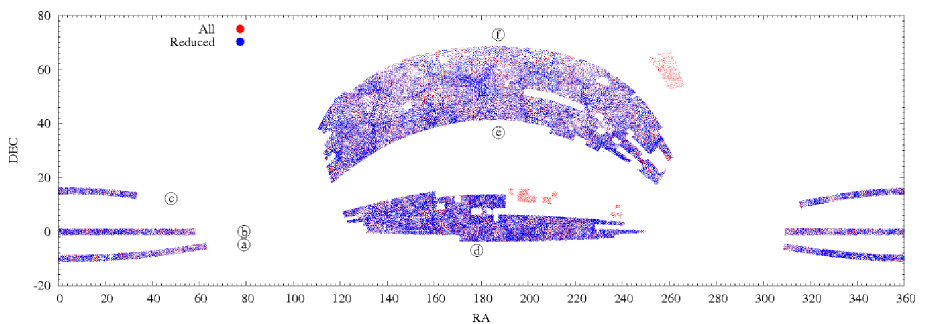
Furthermore, the geometry of the group catalog can be quite complex, introducing difficulties in the process of the reconstruction and during the analysis of the density field. In order to simplify our procedures associated with the complex geometry of the survey, we have made a reduction in the geometry of the halo catalog and worked with groups that are contained inside a compact geometry, removing small slabs or peaks in the border of the window survey. Figure 1 shows in equatorial coordinates the original and final distribution of groups after the geometry reductions.
All this selection criteria applied to the group catalog leaves us with a set of 86128 haloes in the halo catalog for the reconstruction with and 8165 haloes for . Each one of these sets of haloes determine the function necessary for the reconstruction.
Assuming that the luminosity-weighted redshift of each group () corresponds to the redshift of each halo in the halo catalog, we compute the comoving cartesian coordinates for each halo from the coordinates of the associated groups as
| (3) | |||||
where and are the right ascension and declination of each galaxy group in the group catalog and is the comoving distance of the respective halo, given by
| (4) |
with being the speed of light, and is the Hubble constant at present time. Then, our sample of haloes is contained in a set of slices of radius in comoving units.
Finally, for each halo we computed its radius from their masses using Eq. 5 below, assuming that they all are situated at .
The reconstruction of the density field presented in this paper has been done in redshift space, and therefore it must contain redshift space distortions in the coordinates of the haloes coming from the group catalog. However since the reconstruction method is based in haloes, most of the highly nonlinear redshift effect distortions should not be present, and only mildly linear regime effects may be accounted for. As was shown in Wang et al. (2009), this method can be used to make reconstructions of the density field in real space, nevertheless we have decided to work in redshift space since computing properly the effects of the large scale structure on the velocity field requires an isotropically sampled volume. As the sampling geometry of the survey used for the reconstruction (SDSS-DR4) is highly anisotropic, consisting on several slabs, the large empty regions in the volume of the reconstruction will make it unreliable to estimate the influence of the unseen large scale structures on the velocities of the objects in the reconstruction region.
2.3 Numerical Simulations and the estimation of
2.3.1 Halo and domain identification and halo properties
Our method makes use of the masses and positions of haloes taken from the group catalog of the SDSS and convolves it with the mass distribution in and around dark matter haloes estimated from cosmological simulations. It combines results of simulations and observations in a unique effort seeking for a realistic reproduction of the cosmic mass distribution.
In this work we have used a cosmological simulation ran under the standard spatially flat CDM cosmology in a cubic box of 100 with particles and cosmological parameters given by , , and . In order to be fully consistent, these cosmological parameters where intentionally chosen to be the same set of parameters used in the construction of the halo catalog. No further corrections for cosmology have to be considered, reducing in particular the uncertainties in the mass assignment of haloes (see Yang et al. 2007). For the determination of the mass density profiles we used the last snapshot of the simulation at .
Haloes are identified using a FoF algorithm with a linking length of 0.2 times the mean interparticle distance. The minimum number of particles per halo is chosen according to the mass threshold used to do the reconstruction as , where is the mass of a particle in the simulation. We fixed the mass threshold for the reconstruction to be , which results in a minimum number of 637 particles per halo. This value of is slightly smaller than the minimum mass in the halo catalog, and was defined in that way to be able to account for the typical mass distribution of haloes at its low mass end. As can be seen in table 1 the value of is almost at the center of the first mass bin, therefore, no major effect is expected from this choice. This will be also verified later, when we will show the independence of the general properties of the reconstruction on .
For each halo we define its center as the position of the particle with the lowest potential energy. The virial mass of the halo is defined as the mass of the sphere enclosing a mean density equal to , where is the virial density contrast computed using the fitting formula from Brian & Norman (1998) and is the critical density of the Universe. For and the cosmology assumed for this work . The virial radius of the haloes is computed as the radius at which the enclosed mass equals , and is related to this by
| (5) |
The domain of a halo represents the unique region of the Universe that is closest to the halo than to any other. Following Wang et al. (2009) we identify the domain of haloes in the simulation using the particle distribution. The domain of a halo is identified as the region of space containing all particles for which the weighted distance measure between the halo and the particle is minimal across all the population of haloes. It is implicit here that the particle is not bound to any other halo by the FoF procedure and is the distance between the halo of virial radius and the particle.
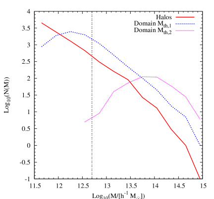
Figure 2 shows the mass function of haloes and their domains for our simulation at the two different mass thresholds = and = . Note that for both lines (haloes and domains) are almost parallel for all masses above , with discrepancies at the low and high mass end. It shows that very massive haloes tend to have more extended and massive domains, while at the low mass end it is clear that low mass haloes may have very small domains or can even have no domain at all. The mass function for shows a higher number of haloes with massive domains. This can be easily interpreted, since using a higher mass threshold implies that less structures are resolved as haloes and therefore more mass is associated to the domain of more massive haloes.
2.3.2 Computing the mean mass density distribution of haloes
Once the virial masses, radii and domains of haloes are determined, we proceed in estimating the mass density distribution associated to each halo. For this step, we bin the haloes in the simulation by mass, each of these mass bins will be called a population of haloes. Then we compute the mean mass distribution for each population from the simulation. See table 1 for a detailed description of the mass binning used in this work.
Assuming that each particle in the simulation box has an associated volume , we computed binning the particle distribution in radial logarithmic bins of width where is the normalized radius at distance from the center of the halo. For a given population with haloes we computed the mean mass density as the ratio of the total mass enclosed in that radial bin from all haloes in the population divided by the volumes of the particles per halo inside the radial bin of width , explicitly
| (6) |
The volume of every particle has been computed using a Delaunay tessellation over the particles in the simulation box (O’Rourke 1998), where the Delaunay tessellation has been computed using the freely available library Qhull (Bradford et al. 1996). As it has been noted in Wang et al. (2009), for a given population, is nothing else than the correlation function between haloes and the mass distribution around them, so the reconstruction method carries implicitly the information of the correlation function of the simulation (and therefore, of the cosmology that has been adopted) through .
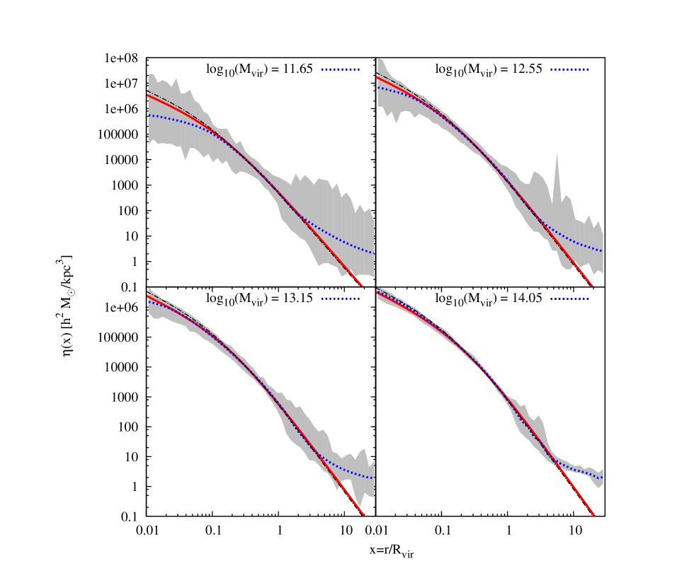
Figure 3 shows the typical density profiles estimated for four different halo populations, compared with the individual density profiles for individual haloes in that population (i.e. we use Eq. 6 for each halo separately) and with the standard NFW profile with a mean concentration parameter as given in Macciò et al. (2008) for a WMAP3 and Muñoz-Cuartas et al. (2010) for a WMAP5 cosmology.
In the figure the grey region shows the scattered distribution for the individual density profiles of haloes. As it was expected, the scatter is larger for the low mass bins. At the scatter is high since low mass haloes have a high scatter of concentration parameters. At the scatter is large due to the many different environments in which the low mass haloes are located. We emphasize that this scatter is not due to resolution effects, since the less massive haloes in this work have been identified with at least 637 particles, this is a high enough number of particles to resolve the density profile (Muñoz-Cuartas et al. 2010, Trenti et al. 2010). Note also in the figure that the mean density profiles approach satisfactorily the NFW shape, even for . The comparison of with the mean density profile for the WMAP3 and WMAP5 cosmologies shows that in principle one could relax the requirement that the simulations used to get must have exactly the same cosmology as the one used to create the halo catalog.
2.3.3 Mass assignment in domains
Now we describe the procedure used to assign masses in the domain of each population of haloes. As will be shown in the next section, haloes may start with an initial guess for its domain mass, but during the reconstruction procedure, depending on the environment where they are located, this initial mass is reduced until a final mass is assigned to the domain of each halo. We use the term “initial mass in domains” in reference to the guessed initial value for the mass in the domain, and “final mass in domains” in reference to the real final mass associated with the domain of the halo after the reconstruction is completed.
Since each halo in the simulation has been assigned to a population, all of the haloes in the same halo population will be characterized by the same mean mass density distribution, and in particular, the same initial mass in their domains. The initial mass in each domain of haloes is computed from the mean density profile as
| (7) |
where for we have used the numerical values obtained from the simulation for each halo population and was set to . For each population was calculated consistently with the value of the mean mass of that population using Eq. 5.
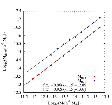
Figure 4 shows how the mass assignment procedure relates the mean mass of the halo population with its mass in the domain as a power law . The normalization constant is close to and for and , respectively, showing that domains of perfectly isolated haloes could be more or less one hundred or one thousand of times more massive than the haloes themselves. This proportionality grows directly with the value of . It is worth to note that this factor of about ten difference in the normalizations is close to the mass ratio between the two different mass thresholds we choose. This difference shows that for a given the mass we ignore in the form of dark matter haloes goes directly to the domains in the form of cosmic background mass.
2.4 Reconstruction
|
| (a) (b) |
|
| (c) (d) |
|
| (e) (f) |
Having all of the ingredients, one can proceed to use Eqs. 1 and 2 to make the reconstruction of the density field using the function describing the positions and masses of the set of haloes from the halo catalog and assigning them to a halo population according to their masses, this will provide the form of and the initial mass in the domain of every halo.
In practice what we do for each halo in is:
-
1.
Assign haloes in to a given halo population according to their masses,
-
2.
Assign an initial mass to the domain of the halo according to its population and assign a total number of sampling particles. To obtain a final reconstruction consistent with the properties of the halo catalog, during the reconstruction, we force the halo to have the same mass inside the virial radius as in the catalog, so the total number of sampling particles is divided in two sets, halo particles and domain particles for each halo of mass and domain mass , and where is the mass of each sampling particle in the reconstruction.
-
3.
Then we generate a particle realization of the density profile at the position of the halo for the particles inside the virial radius (). Once the halo has been realized, we proceed to generate a particle realization of the density profile in the domain of the halo () with particles. In this step, only particles that fall inside the domain of the halo, computed across the complete halo catalog , are accepted to be part of the reconstruction. This step defines the operator introduced in Eq. 2. Here one can see that because of the rejection of the particles outside of the domain of the current halo, the operation can not be interpreted formally as a convolution and can only be defined operationally as we just did. Note that, as was already mentioned, in this step the actual number of particles in the domain and its mass will be different (lower) than the values assumed initially.
An issue to consider during the procedure of reconstruction is related to the border and the geometry of the survey. Although we have made simplifications to the geometry of the distribution of haloes, the SDSS-DR4 and therefore the halo catalog has a geometry that makes it difficult to implement the method. In particular, haloes in the border of the survey have large fractions of totally empty space around them due to the boundary. For these haloes, during the reconstruction, the extension of their domains in that direction will be larger than expected if the unobserved haloes where present in the data in that region. This will represent unphysically the mass distribution in those regions. To avoid these drawbacks we use an auxiliary catalog of haloes filling the empty regions of the survey and forming a thick envelope around the different slabs of the survey. This envelope was built taking haloes from a simulation of box size 1. These haloes are used not to build the reconstruction of the density field around them, but for constraining the extension of the domain of the haloes in the borders of the survey.
3 Results
3.1 General properties
| Name | ||
|---|---|---|
| 13 | 9 | |
| (/) | 11.5 | 12.7 |
| 11.65,…, 0.3dex | 12.85,…, 0.3dex | |
| 86128 | 8165 | |
| 0.496 | 0.496 | |
| Total |
The outcome of the reconstruction procedure just described is a set of particles tracers of the density field distributed according to the mass distribution in haloes and their domains. The resulting particle distribution resembles the particle distribution in N-body simulations. Their positions are constrained by three factors: the positions of the haloes in the halo catalog, their environments and the shape of the mass distribution around halos of a given mass.
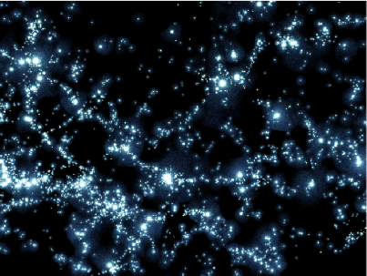
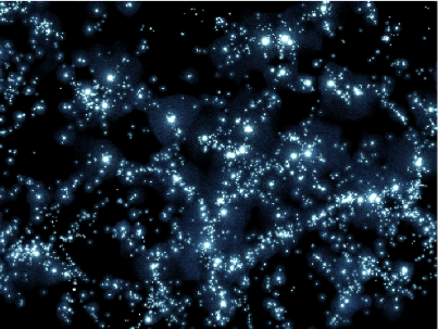
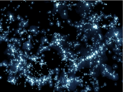
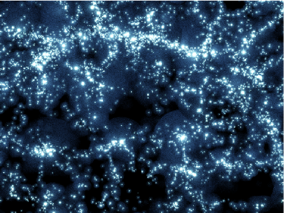
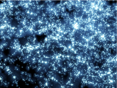
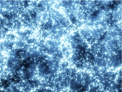
Figure 5 shows slices of the reconstruction
for the different slabs on the survey, as described in the
caption. After a visual inspection it can be clearly seen how the
reconstruction method not only allows for the identification of high
density regions, but also clearly allows the identification of empty
regions. The slices were chosen to be thick enough ( 10) to
enclose a representative number of haloes and to make sure that the
structures (filaments or voids) observed are not due to geometrical
incompleteness of the survey. In panel (d) one can also see a large
structure running almost at the same distance from the origin across
all of the slice, that corresponds to the Great Wall, and just below
it one can see a huge empty region (Gott et al. 2008).
One of the free parameters in the method is the mass threshold used to make the reconstruction. In order to test for the influence of the choice of this value in our results we have run two reconstructions and analyses using two different mass thresholds, the first one, corresponds to a halo mass of threshold , while the second one is almost ten times larger, =. Table 1 summarizes all the parameters used to run both reconstructions.
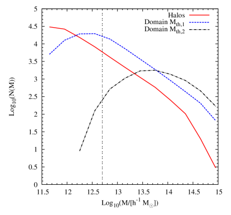
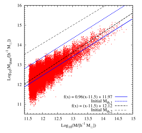
Figure 6 shows the initial and final mass assignment in domains of haloes of mass . The scatter plot shows the distribution of masses for haloes in the realization with . The step-like shape in the distribution of points is due to the discreteness in the assignment of mass in domains for haloes in a given population. The solid blue line shows a linear fit to the data for . The blue dashed line shows the initial mass assigned to domains of haloes of mass for that mass threshold. The difference between the initial and final mass assigned is due to the overlapping of the domains during the reconstruction that reduces the mass in domains. For the power law relation between the final mass in domains and has the same power law index as the one for the initial mass assignment, implying that on average, for a given halo mass, the final mass assigned in domains is a factor of times lower than initially assigned. For the reconstruction with , the final - relation has a slightly different power index, this will imply a mass dependence between the ratio of the initial and final mass in domains, giving more mass in domains to more massive haloes. However the difference is very small, and the final mass in domains in haloes in the reconstruction is around a factor of times smaller than initially assigned.
Figure 7 shows the mass function of haloes (number of haloes with masses between and ) and domains. The red solid line shows the mass function for the halo catalog used in the reconstruction, while the blue dashed and black dot-dashed lines are the mass functions for domains in the reconstructions for and . The mass function for haloes is the same for both realizations, only that for it is truncated at the low end at , as shown by the vertical line in the Figure. It can be seen that higher values of lead to higher masses assigned to domains, as was expected from Figure 4. One can see from the Figure that the mass function for domains is always larger than the one for haloes except for masses below for and for , where the number of haloes with domains of mass decreases and even it can be possible to have haloes with domains less massive than the halo itself. Such a behavior is expected for haloes close to . Note also that the mass functions for the domains cross each other at and for a given mass, the number of haloes with massive domain is higher for relative to . The higher amplitude of the domain mass function for may be responsible for the different slope observed in Figure 6 for the mean mass halo-domain relation. Note also the similarity of this plot with the one shown in Figure 2 where we show the equivalent quantities for the haloes in the simulation.
A point worth to be verified in our implementation of the method is the assumption of the correspondence of the density profiles computed for haloes in the simulation in real space, with haloes in the survey that are in redshift space. As pointed out in Wang et al. (2009), since the method is based on individual haloes, each associated to a group of galaxies, all the strong nonlinear redshift distortions are absorbed in to the selection of individual haloes for the reconstruction. Mildly nonlinear and linear redshift distortions should still exist anyway in the halo catalog, and we expect them to be not strong enough to affect the final reconstruction.
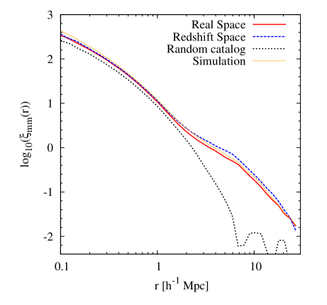
To test this assumption, we compare two reconstructions of the mass density field using the halo catalog taken from the cosmological simulation described in section 2.3. One of the catalogs has the original positions of the haloes in real space, while for the other one we pick a halo close to the center of the simulation box. Relative to this halo we recompute the positions of all other haloes in redshift space according to their peculiar velocities, mimicking the redshift space distortions. Then we build the reconstructions using in both cases the same set of functions , computed in real space. We compute the correlation function for both reconstructions following the procedures shown in section 3.3 and find very small differences between the reconstructions in real and redshift space. As can be seen in Figure 8, the effect of using the real space density profiles makes the haloes to be slightly more clustered on scales . The clustering pattern at scales larger than is dominated by the large scale clustering of haloes, while for scales shorter than the shape of the correlation function is dominated by the typical mass distribution of haloes in real space. We conclude after this test, that if well, it is true that the use of the density profiles computed in real space is not fully consistent with its use on a halo catalog that is built in redshift space. However the fact of the use of haloes as centers to convolve the density distribution reduces the effect of the redshift distortions to levels we consider acceptable.
It is important to note that the method can be implemented in real space, as it has been shown in Wang et al. (2009). In the current work we just focus on the redshift space reconstruction and reserve for further papers the implementation of the method in real space.
3.2 Mean mass density
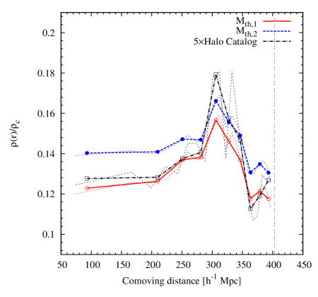
Another quantity that can be estimated from the reconstruction is the mean mass density in the volume of the survey. We compute it in radial comoving shells of width centered in the center of the survey. For this we use a procedure similar to the one used in section 2.3.2 to compute the value of for each population of haloes. First we associate a volume to each particle in the reconstruction using a Delaunay tessellation, then we group the particles in radial bins of width and compute the density in that bin as the sum of the mass of the particles inside the bin divided by the total volume, the last, computed as the sum of the volumes of all the particles inside that bin. The width for the radial bins is fixed such that each bin contains the same spherical volume. We compute the density distribution for the halo catalog using the same procedure but in this case the mass in each spherical bin is the sum of the masses of the haloes inside the bin.
Figure 9 shows the result of the density estimate as a function of comoving distance. We used 10 and 20 radial bins and no major differences were found for the values of except for the halo catalog where the peak initially seen at 300 is resolved in two different peaks at 300 and 325 . This double peak is also seen in the density distribution of the two reconstructions but the difference is not as drastic as for the halo catalog. As one expects, the radial mass density changes with distance but remains close to the mean value, being nearly constant for the first 200 but presenting a peak at 310. That peak is associated with the presence of the Great Wall of galaxies which makes the local mass density to increase by about 20% relative to the mean density. Beyond the Great Wall, the density drops below the mean value again mainly because right behind the Great Wall is the border of our reconstruction.
The total mean mass density in each case is 0.13, 0.14 and 0.03 for , and for the halo catalog respectively. Clearly the mean mass density for the halo catalog is around a factor of five times lower than for the (reference) reconstruction with . These values for the mean density are off by factors of 1.8, 1.66 and 8.7 relative to the cosmological mean mass density of 0.24. Although these results are acceptable for the mean cosmic mass we computed in our reconstruction without the assumption of any bias, we assume the difference between the reconstructions and the expected values of the mean density by a factor of 2 are due mainly to the masses assigned to haloes in the halo catalog.
To verify this affirmation, and to test that the disagreement in the values of the mean mass density in the reconstruction is not due to the method or our implementation, we run a test using a cosmological simulation of 1 volume. From the catalog of haloes in that simulation we take a sample of haloes with the same geometry and selection criteria we used to build the halo catalog from the group catalog of the SDSS, but in this case assuming that the halo mass is the one computed from the particle distribution in the simulation. Then we ran the reconstruction using that set of haloes and compute its mean density. As a result, we obtain for this test reconstruction a mean density of , in very good agreement with the simulation input. This verifies that the factor of around 2 difference in the mean mass density we see in our reconstructions of the density field is not due to the reconstruction method, but is likely related to the properties of the group catalog and potentially due to the presence of cosmic variance.
3.3 Correlation functions
Figure 10 shows the mass correlation function for the reconstructions with and and the correlation function for the underlying halo catalog for the two mass thresholds. To estimate the correlation functions in the reconstructions we take from each of them random subsamples of data points of particles. We use those samples to compute the two point correlation function with an uniform random catalog with equal number of random points. The selection of the size of the sample of points should not affect the estimated correlation function. This is clear if one thinks that reducing the particle resolution of the reconstruction, it will end up consisting on a lower number of particles (i.e. as small as if one chooses the appropriated value for ) that by construction should follow the same density distribution as the reconstruction with a high resolution, therefore, giving rise to the same correlation function, only affected in the low scales by the low resolution of the reconstruction. However, to test for the response of the estimates of the correlation function to the arbitrariness of the number of points of the subsample , we repeate the procedure with and . We found no major dependence in the correlation function on . Figure 10 shows that the reconstruction clearly exhibits the two terms of the correlation function (Zehavi et al. 2004, Hayashi & White 2008), the one-halo term dominating the correlation function up to and the halo-halo term dominating for .
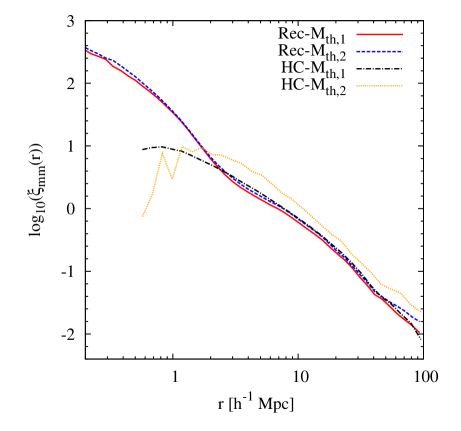
As it has been already shown (Wang et al. 2008, Hayashi & White 2008) more massive haloes are more strongly clustered. It can be seen in Figure 10 for the correlation functions of haloes in the halo catalog for and where is large for the most massive population of haloes . It is very interesting to note that, independent on the biasing of the halo population used to perform the reconstruction, the correlation function of the mass distribution in the reconstruction is almost the same. We find that our reconstructions of the cosmic mass density field are bias free in the sense that although there is not explicit assumption about bias, the reconstruction method converges for the mass clustering pattern (mass correlation function) for different values of . This result is also a proof of the consistence of the reconstruction, since it approaches very well the clustering pattern of the underlying cosmological model, as it is shown in Figures 8 and 10.
We have to explore the reason of the small deviation in for . In principle it can be due to fact that computing for a mass threshold as high as requires the use of simulations with a larger volume than the one used in this work to allow a better sampling of the environment of haloes on the very large scales.
We try to identify the scales where the results of our reconstructions are dominated by the priors of the method, specifically, by the shape of the functions . We take the catalog of haloes from the simulation, and replace the original positions of the haloes by random positions uniformly distributed into the volume of the box. This procedure should erase all physical relation between haloes in the box while keeping the same mass function for the haloes in the volume. Then we ran a reconstruction of the mass density field using this artificial halo catalog and estimate the correlation function of the reconstruction. After this experiment we observe that only the one-halo term in the correlation function is dominant, as can be seen in Fig. 8. Comparing this correlation function to the one obtained from the reconstructed density field for the simulation, we conclude that the reconstruction method dominates in the scales of . This result was expected, since there is no information from the observations for these small scales. For scales larger than the method preserves the original clustering pattern, which is indication that there is no major influence on the result at these scales.
3.4 Statistics of counts in spheres
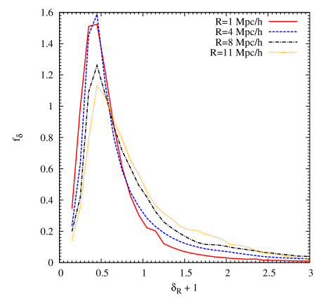
Finally, we study the mass in the reconstruction through the particle distribution, computed in spheres of radius . In order to avoid the inconvenients related with the geometry of the survey, we study the count in cells for the mass distribution using a subsample volume. We take two cubic volumes of side length 60 from the north cap of the survey and the reconstruction with , and compute the mass distribution in spheres of radius from the particles of the reconstruction. The subsamples containe particles from the realization, and random points were used to compute the counts in spheres. Figure 11 shows the distribution of the mean mass density contrast, , in spheres of radii . The mean mass density contrast, , is defined as
| (8) |
where is the mean mass density in the reconstruction and is the mean mass density in the sphere. As expected, due to the non-linearity of the scales studied, the distributions are not Gaussian. However it can be seen that the distributions have a skewed log-normal like shape, and broadens and moves to the right (tending to 1) for increasing values of . This behavior is be expected (Coles & Jones 1991) if one assumes that going to larger values of , the mean density contrast should become more linear, therefore closer to be Gaussian and having a mean
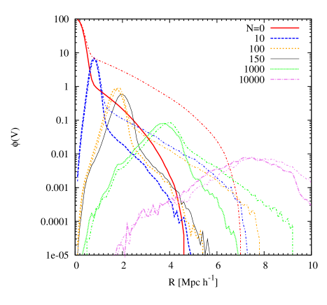
Following Maurogordato & Lachieze-Rey (1987) we computed the number of particles inside all of the random spheres drawn inside the cubic box of 60 side. Then we compute the probability of a sphere of radius to contain particles, , as
| (9) |
where
| (10) |
is the sum of all the spheres containing particles. Figure 12 shows the fraction of spheres of radius containing particles for and . Note that this number of particles can be translated to mass, so, Figure 12 shows the fraction of spheres of radius containing masses of 0, , , and respectively. To be able to compare with the mean density predicted by the cosmological model, we have accounted for the fact that the reconstruction has a mass assignment biased by a factor of relative to the true cosmic mass, as was shown in the previous sections. To test for the effects of the cosmic variance introduced by the small size of the boxes used (60), we plot in thin lines (thin dot-dashed lines) the same quantity, , for a second subbox of the same size. It can be clearly seen that for both boxes the shape of the distribution is the same, the peaks are located nearly at the same radius but they are broader for the second subbox. These differences are simply due to the second subbox to be taken from a region with a lower mean density than the first one.
As it can be seen from the Figure 12, requiring the spheres to be totally empty forces the distribution to be peaked at , as one would expect in that case it will be more probable for the smaller spheres to be empty. Requiring spheres to contain shows that it is more probable to find them having a radius of and spheres containing will be found more frequently in spheres of radius . Of special interest is to see what is the most probable radius of the sphere containing a mass of (solid black line in Figure 12). As it can be seen in the Figure, that amount of mass can be found most probably in spheres of radius . This result is another independent verification of the ability of our reconstruction to fit the expectations from the models, since for and the cosmology assumed for this work, the characteristic non-linear mass is , and the related radius , in very good agreement with the previous result. This also supports the fact that the mismatch in the mean mass densities shown in the previous sections is mostly due to the mass assumed for the haloes from the group catalog.
3.5 Characterization of environments
We now investigate the morphological classification of the cosmic web in our reconstruction of the density field. Following Forero-Romero et al. (2009) we classify the different environments of the reconstructed density field in peaks, filaments, sheets and voids, according to the the eigenvalues of the deformation tensor of the cosmic mass distribution. To this end, we compute the smoothed density field arising from the particle distribution on a regular cubic grid of size 1 and cells, and fill the empty regions of the survey with a set of particles randomly distributed with a mean mass density equal to the mean mass density of the reconstruction. Then we compute the potential of the smoothed density field in the grid and from it the deformation tensor
| (11) |
We classify the environment computing the eigenvalues of the deformation tensor for every cell and compare them with a threshold as a confidence value for the choice of the classification. The type of environment assigned to each cell is determined by the number of eigenvalues above . Such a procedure will allow us to study in detail not only the geometrical properties of the mass distribution through the cosmic web, but it will also provide a direct link between environments in the volume of the reconstruction and the properties of the galaxies residing in these environments.
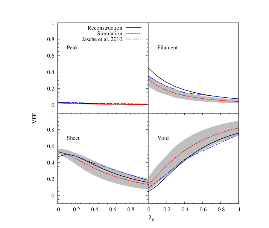
Figure 13 shows the volume filling fractions (VFF) for each environment characteristic computed for the reconstructed density field and for a cosmological simulation, for a comparison. For the simulation we used the 1 simulation already mentioned. In the volume of that simulation we took a piece with the same geometry of the survey and produced an equivalent background distribution. As can be seen in Figure 13, the volume filling fractions for peak and sheet environments in the reconstruction follows very well the same behavior observed for the simulation. Differences are observed for filaments and voids. As it has been shown in Forero-Romero et al. (2009), the differences may be due to fluctuations induced by cosmic variance. One can verify this by comparing our VFF with the ones obtained by Jasche et al. (2010) for the reconstructed density field of the SDSS-DR7 using a completely different approach. The agreement for both estimates of the VFF for roughly the same region of the universe indicates that the observed differences relative to the simulation are mostly due to cosmic variance.
Note that the volume filling fractions for filaments, peaks and sheets decrease with the increase of . That behavior is be expected since increasing the value of decreases the probability for the eigenvalues of to be larger than the given , then increasing the number of cells classified as voids and necessarily decreasing the number of cells classified as the other environments.
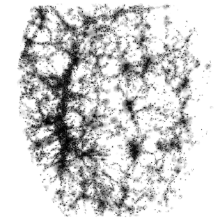
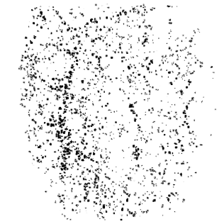
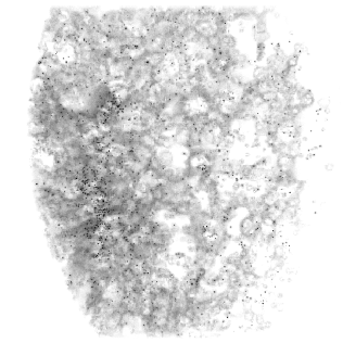
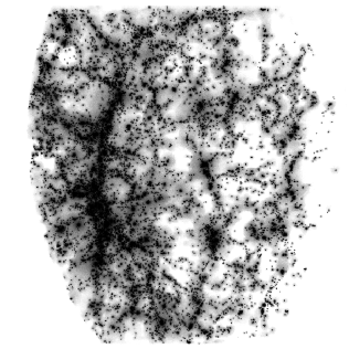
Figure 14 presents a visual impression of the results of the classification of the cosmic network in our reconstruction for (see Forero-Romero et al. 2009 for details in the selection of this value). The Figure shows a piece of the survey of and thick, enclosing the Sloan Great Wall. The panels show how the classification recognizes filaments, peaks and sheets in the reconstruction. It can be clearly seen how the peaks are distributed following the structure of the filaments. Note also that although there are peaks inside the regions classified as filaments, which is partly due to the discreteness of the grid used to compute the eigenvalues of , but also due to the inherent nature of haloes to be located in filaments, the filaments are characterized by the smoothly extended mass associated to the environment of the haloes. The last panel shows together the regions classified as peak and filaments, and it can be clearly seen where are the empty regions (voids) surrounded by filaments.
4 Discussion and Conclusions
We have presented the implementation of a halo based reconstruction of the cosmic mass density field. The method combines the results of observations and simulations, convolving the mass density distribution in and around dark matter haloes computed from N-body simulations with the coordinates of haloes of a given mass identified in the group catalog of a galaxy survey. We have used the group catalog of Yang et al. (2007) built from the SDSS-DR4 together with high resolution simulations of the formation of the structure in the standard spatially flat CDM model.
The reconstruction method produces a distribution of points sampling the cosmic mass density field that is determined by the mass and position of the dark matter haloes in the halo catalog, convolved with the estimated typical density distribution of mass in haloes and their environments. The final particle distribution resembles that obtained from cosmological simulations, and as the reconstruction method does not requires the definition of any scale length, it provides a high dynamical resolution. Tracer particles are more probably found in high density regions, however the adaptivity of the method allows to sample also the low density regions of the cosmic web.
Instead of imposing a smoothing length, the resolution and smoothness of the method is limited by two factors, the value of the mass threshold and the mass of the sampling particles . The resolution of the reconstruction is set by the choice of the mass threshold . Using lower values for the mass threshold produce a more detailed reconstruction of the density field at small scales. The selection of the mass threshold plays a role similar to the smoothing length in standard grid techniques of computing the density field, like cloud in cell (CIC), where structures below the threshold value (smaller than the smoothing length in the case of the CIC method) are erased and smoothed out in the density field. A key result is that, as was shown throughout the paper, the choice of the value of the mass threshold does not affect the global properties of the reconstructed density field.
The other parameter defining the the smoothness of the reconstruction is the mass of the particles used to sample the density field, . Low mass sampling particles produce a smooth and more well defined sampling of the density field, specifically in the case of haloes with masses close to the mass threshold . In general has to be lower than , to allow the particle distribution to reliably reproduce the mass associated with haloes of masses close to the mass threshold.
It is worth to note that the reconstruction method is based on the concept of individual haloes, that is, main haloes in the language used in cosmological simulations. Due to observational constraints, this method would be better to be used in populations of haloes in a mass range above , where is it is possible to reliably identify complete samples galaxies and groups of galaxies associated to haloes down to this mass value.
As it has been shown in section 3, the shape of the correlation function for our reconstructions using two different values of converges to similar values at almost all scales. From this result and the fact that the method does not make any explicit assumption about biasing, the resulting reconstructions are a very suitable tool to address studies of galaxy properties and their relation with the large scale density field. The known effect of biasing, for haloes of different mass is introduced in a natural way in the reconstruction through the functions .
A drawback of the method (and of any reconstruction method in general) is that it is strongly dependent on the properties of the catalog of haloes as well as on the details of the typical mass distribution in and around of haloes extracted from the simulations. The quality of the observations, and in particular, the properties of the halo catalog, have an influence on the quality of the reconstruction. It was shown that the mass assigned to haloes in the halo catalog gives values of the mean cosmic density that are off by a factor of around 2. Clearly better estimates of the masses of haloes may produce a better constraint. Despite the discrepancy, we see this result as motivating and as a good starting point in the improvement on the methods used to assign masses in the halo catalog like the one presented by Yang et al. (2007). On the other hand, as we have shown, we can assume the masses in the halo catalog to be off by the same factor of as the density. This value is in complete agreement with the measured scatter for the mass assigned to haloes in the group catalog (Yang et al. 2008, Wang et al. 2008). We believe that the volume of the survey have no influence on this mismatch since it is totally independent on any assumption besides the cosmological parameters.
It is also true that assuming the typical density distribution of mass from simulations will make the method not appropriate to extract further cosmological information from the mass distribution in the halo catalog. Such an assumption is similar to assuming a power spectrum shape, as done in methods like the Wiener filter techniques. As it has been already mentioned, the power of the method relies on its physical simplicity, directly connected to the ideas of the halo model, and it is best suited to make studies of the properties of the mass distribution: large scale environments and environmental effects on galaxy formations, and problems where there is a pre-stablished cosmological model, like the realization of constrained simulations.
Besides the aforementioned sources of error coming from the observations, we have shown different potential sources of error in our reconstruction, and we have shown where the reconstruction is more strongly dominated by the data or by the priors of the method. Nevertheless is difficult to quantify the degree of error introduced in the reconstruction. We have estimated the amount of deviation between the expected and reconstructed mean mass density. This number may be taken partially as an estimation for the mean error in the reconstruction. Analysis in the clustering pattern give also information about the degree of effects introduced by the method at different scales. But in general, as far as it has been shown in this and in previous implementations of the method, there is not yet a formal model to properly estimate the errors of the reconstructed density field in a given point, and will be part of further research to study in deep this issue.
To check for the consistency of our results we have made an exhaustive study of the properties of the reconstructed density field. We have shown that the reconstructed density field reproduces the mass correlation function. It clearly shows the two regions associated to the one halo and two halo terms. Comparing the correlation function for our reconstruction with the one for the halo catalog, we see that the amplitude of the correlation function is in agreement with the expected clustering at large scales, and by construction it reproduces the small scale clustering. More interesting is that it shows the bias-free nature of the method in the mass correlation function. We computed the properties of the mass distribution in spheres and verified the way the mass distribution follows a skewed, log-normal like distribution when computed at small scales. As expected (Coles & Jones 1991), this distribution broadens and shifts to for larger smoothing radii.
The classification of the cosmic web for the reconstructed density field also offered consistent results with the theoretical expectations. The volume filling fraction of the different characteristic environments (filaments, sheets, peaks and voids) in the reconstruction match the ones obtained from simulations. Only small differences within the expected cosmic variance are observed (Forero-Romero et al. 2009).
Reconstructions of the density field as the one we have shown provide a way to map directly the cosmic mass distribution from the halo catalogs identified in the surveys without the necessity to assume any functional form for the bias factor. Provided that the data fulfills a minimum completeness requirements, coupling this method of reconstruction of the density field with a reconstruction of the velocity field will offer the opportunity of computing real space density fields. This will give us detailed information about the velocity field of the observed volume, information valuable to quantify and map the effects of the redshift space distortion, and usable to test the dynamics of the local neighborhood (Lavaux et al. (2010a), Strauss & Willick 1995).
Furthermore, the results of the cosmic web classification obtained with the help of the reconstructed density field can be used to study the properties of the galaxies in the large scale environment, not only in their close environment (Tempel et al. 2010, Weinmann et al. 2009, 2008, Wang et al. 2008, Park et al. 2007).
The ability of the method to trace the mass distribution in an adaptive way, coupled with the ability to work in real space, makes the method a good choice to produce appropriate and high resolution density fields to be used as background for time machines used in the realization of constrained simulations structure formation (Kolatt et al. 1996, Martinez-Vaquero et al. 2009, Gottlöber et al. 2010, Lavaux et al. 2010b, Nuza et al. 2010).
Acknowledgments
J.C.M. was supported by the German Science Foundation under the grant MU-1020/6-4. We thank to Sebastian Nuza and Stefan Gottlöber for useful comments to the manuscript, and to the referee for his/her comments that helped to improve the presentation of this paper. Part of the reconstruction and the analysis has been performed in the Altix Supercomputer of the Leibniz Rechenzentrum (LRZ) Munich. The simulation of the box 1 used for our tests has been performed by A. Klypin and S. Gottlöber at LRZ Munich within the German AstroGrid-D project.
References
- Berlind et al. (2006) Berlind, A. A., et al. 2006, ApJs, 167, 1
- Qhull (1996) Bradford, C. B., Dobkin, D. P., Huhdanpaa, H., 1996, ACM Trans. Mat. Soft., 22, 469
- Bryan & Norman (1998) Bryan, G. L., & Norman, M. L. 1998, ApJ, 495, 80
- Colless et al. (2001) Colless, M., et al. 2001, MNRAS, 328, 1039
- Coles & Jones (1991) Coles, P., & Jones, B. 1991, MNRAS, 248, 1
- Cooray & Sheth (2002) Cooray, A., & Sheth, R. 2002, Phy. Rep., 372, 1
- Crook et al. (2007) Crook, A. C., Huchra, J. P., Martimbeau, N., Masters, K. L., Jarrett, T., & Macri, L. M. 2007, ApJ, 655, 790
- Davis & Djorgovski (1985) Davis, M., & Djorgovski, S. 1985, ApJ, 299, 15
- Erdoğdu et al. (2004) Erdoğdu, P., et al. 2004, MNRAS, 352, 939
- Erdoğdu et al. (2006) Erdoğdu, P., et al. 2006, MNRAS, 373, 45
- Fisher et al. (1995) Fisher, K. B., Lahav, O., Hoffman, Y., Lynden-Bell, D., & Zaroubi, S. 1995, MNRAS, 272, 885
- Forero-Romero et al. (2009) Forero-Romero, J. E., Hoffman, Y., Gottlöber, S., Klypin, A., & Yepes, G. 2009, MNRAS, 396, 1815
- Gott et al. (2008) Gott, J. R., III, et al. 2008, ApJ, 675, 16
- Gottloeber et al. (2010) Gottloeber, S., Hoffman, Y., & Yepes, G. 2010, arXiv:1005.2687
- Hahn et al. (2007) Hahn, O., Porciani, C., Carollo, C. M., & Dekel, A. 2007, MNRAS, 375, 489
- Hayashi & White (2008) Hayashi, E., & White, S. D. M. 2008, MNRAS, 388, 2
- Huchra et al. (1983) Huchra, J., Davis, M., Latham, D., & Tonry, J. 1983, ApJs, 52, 89
- Huchra (2000) Huchra, J. P. 2000, Cosmic Flows Workshop, 201, 96
- Jasche et al. (2010) Jasche, J., Kitaura, F. S., Wandelt, B. D., & Enßlin, T. A. 2010, MNRAS, 406, 60
- Jasche et al. (2010) Jasche, J., Kitaura, F. S., Li, C., & Enßlin, T. A. 2010, MNRAS, 409, 355
- Kitaura et al. (2009) Kitaura, F. S., Jasche, J., Li, C., Enßlin, T. A., Metcalf, R. B., Wandelt, B. D., Lemson, G., & White, S. D. M. 2009, MNRAS, 400, 183
- Kolatt et al. (1996) Kolatt, T., Dekel, A., Ganon, G., & Willick, J. A. 1996, ApJ, 458, 419
- Kovač et al. (2010) Kovač, K., et al. 2010, ApJ, 708, 505
- Lavaux et al. (2010) Lavaux, G., Tully, R. B., Mohayaee, R., & Colombi, S. 2010a, ApJ, 709, 483
- Lavaux (2010) Lavaux, G. 2010b, MNRAS, 406, 1007
- Macciò et al. (2008) Macciò, A. V., Dutton, A. A., & van den Bosch, F. C. 2008, MNRAS, 391, 1940
- Martinez-Vaquero et al. (2007) Martinez-Vaquero, L. A., Yepes, G., & Hoffman, Y. 2007, MNRAS, 378, 1601
- Martinez-Vaquero et al. (2009) Martinez-Vaquero, L. A., Yepes, G., Hoffman, Y., Gottlöber, S., & Sivan, M. 2009, MNRAS, 397, 2070
- Maurogordato & Lachieze-Rey (1987) Maurogordato, S., & Lachieze-Rey, M. 1987, ApJ, 320, 13
- Mo & White (1996) Mo, H. J., & White, S. D. M. 1996, MNRAS, 282, 347
- Mohayaee et al. (2006) Mohayaee, R., Mathis, H., Colombi, S., & Silk, J. 2006, MNRAS, 365, 939
- Muñoz-Cuartas et al. (2011) Muñoz-Cuartas, J. C., Macciò, A. V., Gottlöber, S., & Dutton, A. A. 2011, MNRAS, 411, 584
- Nuza et al. (2010) Nuza, S. E., Dolag, K., & Saro, A. 2010, MNRAS, 407, 1376
- O’Rourke (1998) O’Rourke, 1998, Computational Geometry in C. Cambridge University Press.
- Park et al. (2007) Park, C., Choi, Y.-Y., Vogeley, M. S., Gott, J. R., III, & Blanton, M. R. 2007, ApJ, 658, 898
- Percival et al. (2010) Percival, W. J., et al. 2010, MNRAS, 401, 2148
- Reid et al. (2009) Reid, B. A., Spergel, D. N., & Bode, P. 2009, ApJ, 702, 249
- Schaap & van de Weygaert (2000) Schaap, W. E., & van de Weygaert, R. 2000, A&A, 363, L29
- Shectman et al. (1996) Shectman, S. A., Landy, S. D., Oemler, A., Tucker, D. L., Lin, H., Kirshner, R. P., & Schechter, P. L. 1996, ApJ, 470, 172
- Strauss & Willick (1995) Strauss, M. A., & Willick, J. A. 1995, Phy. Rep., 261, 271
- Tago et al. (2008) Tago, E., Einasto, J., Saar, E., Tempel, E., Einasto, M., Vennik, J., M’uller, V. 2008, A&A, 479, 927
- Tago et al. (2010) Tago, E., Saar, E., Tempel, E., Einasto, J., Einasto, M., Nurmi, P., & Heinämäki, P. 2010, A&A, 514, A102
- Tegmark et al. (2004) Tegmark, M., et al. 2004, Phys. Rev. D., 69, 103501
- Tempel et al. (2010) Tempel, E., Saar, E., Liivamägi, L. J., Tamm, A., Einasto, J., Einasto, M., Müller, V. 2010, arXiv:1012.1470
- Trenti et al. (2010) Trenti, M., Smith, B. D., Hallman, E. J., Skillman, S. W., & Shull, J. M. 2010, ApJ, 711, 1198
- Wang et al. (2009) Wang, H., Mo, H. J., Jing, Y. P., Guo, Y., van den Bosch, F. C., & Yang, X. 2009, MNRAS, 394, 398
- Wang et al. (2008) Wang, Y., Yang, X., Mo, H. J., van den Bosch, F. C., Weinmann, S. M., & Chu, Y. 2008, ApJ, 687, 919
- Weinmann et al. (2009) Weinmann, S. M., Kauffmann, G., van den Bosch, F. C., Pasquali, A., McIntosh, D. H., Mo, H., Yang, X., & Guo, Y. 2009, MNRAS, 394, 1213
- Wen et al. (2009) Wen, Z. L., Han, J. L., & Liu, F. S. 2009, ApJs, 183, 197
- White (2001) White, M. 2001, A&A, 367, 27
- Yang et al. (2007) Yang, X., Mo, H. J., van den Bosch, F. C., Pasquali, A., Li, C., & Barden, M. 2007, ApJ, 671, 153
- York et al. (2000) York, D. G., et al. 2000, AJ, 120, 1579
- Zehavi et al. (2004) Zehavi, I., et al. 2004, ApJ, 608, 16