Generation of two identical photons from a quantum dot in a microcavity

Abstract

We propose and characterize a two-photon emitter in a highly polarised, monochromatic and directional beam, realized by means of a quantum dot embedded in a linearly polarized cavity. In our scheme, the cavity frequency is tuned to half the frequency of the biexciton (two excitons with opposite spins) and largely detuned from the excitons thanks to the large biexciton binding energy. We show how the emission can be Purcell enhanced by several orders of magnitude into the two-photon channel for available experimental systems.

Sources of pairs of identical photons are fundamental devices in quantum metrology Nagata et al. (2007), quantum communication and cryptography Simon et al. (2007); Cirac et al. (1997); Duan et al. (2001), linear-optics quantum computation Kok et al. (2007); Lanyon et al. (2008), and even for fundamental tests of quantum mechanics like hidden variables interpretations Aspect et al. (1982); Collins et al. (2002). A number of devices have been proposed and experimentally demonstrated with atomic gases Thompson et al. (2006) or nonlinear crystals Nagata et al. (2007). The realization of such devices, however, is a highly nontrivial task since, in order to be useful, the generated photons need to be almost identical, extremely narrow-band and be generated with an extremely high repetition rate. Some of us and coworkers have recently proposed a scheme based on a single quantum dot embedded in a microcavity del Valle et al. (2010), which theoretically fulfils all the above requirements and, moreover, is particularly promising for scalable technological implementations. The principle relies on the biexciton (the occupation of the quantum dot by two excitons of opposite spins) being brought in resonance with twice the cavity photon energy. Thanks to the large biexciton binding energy, single-photon processes are detuned and are thus effectively suppressed, while simultaneous two-photon emission is Purcell enhanced. This effect has been recently demonstrated experimentally Ota et al. (2011). In the experiment, as in the initial proposal del Valle et al. (2010), the signature for the two-photon emission is a strong emission enhancement of the cavity mode when hitting the biexciton two-photon resonance. Because of incoherent excitation used in both the theoretical proposal and its experimental realization, the quantum character of the two-photon emission is not directly demonstrated nor quantified . Here, we upgrade to a configuration that is nowadays experimentally accessible, where the quantum dot is initially prepared in a pure biexciton state Dousse et al. (2010); Stufler et al. (2006); Flissikowski et al. (2004), and analyze in details the underlying microscopic mechanisms, demonstrating the perfect two-photon character of the emission beyond a mere enhancement at the expected energy. We show how the two-photon state is created by the system in a chain of virtual processes that cannot be broken apart in physical one-photon states. Our understanding is analytical and allows for optimisation of a practical setup, enabling the realization of a practical source of two simultaneous and indistinguishable photons in a monolithic semiconductor device.

The characteristic spectral profile of the cavity-assisted two-photon emission is shown in Fig. 1, with a central peak that is strongly enhanced at the two-photon resonance, corroborating its two-photon character, and surrounded by standard (single-photon) de-excitation del Valle et al. (2010); Ota et al. (2011). The photon-pair peak is spectrally narrow and isolated from the other events, that can never be completely avoided, so the source is appealing on practical grounds. The Hamiltonian of the system reads del Valle et al. (2010):

$$H(t)=(\omega_{a}-\omega_{\mathrm{L}})a^{\dagger}a+\sum_{i=\uparrow,\downarrow}(\omega_{\mathrm{X}}-\omega_{\mathrm{L}})\sigma^{\dagger}_{i}\sigma_{i}-\chi\sigma^{\dagger}_{\uparrow}\sigma_{\uparrow}\sigma^{\dagger}_{\downarrow}\sigma_{\downarrow}\\ +\sum_{i=\uparrow,\downarrow}\Big{[}g_{i}(a^{\dagger}\sigma_{i}+a\sigma^{\dagger}_{i})+\Omega_{i}(t)(\sigma_{i}+\sigma^{\dagger}_{i})\Big{]}\,,$$ (1)

where we have included $i=\uparrow,\downarrow$ the spin-up and spin-down degrees of freedom for the excitonic states $\sigma_{i}$ (fermions) with common frequency $\omega_{\mathrm{X}}$ and $a$ the cavity field annihilation operator (boson) with frequency $\omega_{a}$. The cavity mode can have a strong polarization, say linearly polarized in the horizontal direction for a photonic crystal, a case we shall assume in the following. The biexciton binding energy $\chi$ allows to bring the biexciton energy $\omega_{\mathrm{B}}$ in resonance with the two-photon energy while detuning all other excitonic emissions from the cavity mode. It is red (blue) shifted if the biexciton is “bound” (“antibound”), giving rise to a positive $\chi>0$ (negative $\chi<0$) binding energy $\chi=2\omega_{\mathrm{X}}-\omega_{\mathrm{\mathrm{B}}}$. Our scheme works with both the bound and antibound biexciton. Without loss of generality, we assume $\chi>0$, with the added advantage of being less affected by pure dephasing and coupling to phonons, that we neglect Machnikowski (2008). This binding energy is typically large ($\chi\approx$400\text{\,}\mathrm{\SIUnitSymbolMicro eV}$$) as compared to splittings between excitonic states ($\approx$10\text{\,}\mathrm{\SIUnitSymbolMicro eV}$$) Ota et al. (2011), which is ideal for our purpose. We will assume an equal coupling of both excitons to the linearly polarized mode of the cavity, $g_{\uparrow}=g_{\downarrow}=g/\sqrt{2}$, and take $g$ as the unit in the remaining of the text. The Hilbert space of the quantum dot is spanned, in its natural basis of circularly polarised states, by the ground $\left|\mathrm{G}\right\rangle$, spin-up $\left|\uparrow\right\rangle$, spin-down $\left|\downarrow\right\rangle$ and biexciton $\left|\mathrm{B}\right\rangle$ states. In the linearly polarised basis, the excitonic states are $\left|\mathrm{H}\right\rangle=(\left|\uparrow\right\rangle+\left|\downarrow\right\rangle)/\sqrt{2}$ and $\left|\mathrm{V}\right\rangle=(\left|\uparrow\right\rangle-\left|\downarrow\right\rangle)/\sqrt{2}$. The dot-cavity joint Hilbert space includes the photonic number $n$: $\left|j,n\right\rangle$, where $j=\mathrm{G}$, $\mathrm{V}$, $\mathrm{H}$ and $\mathrm{B}$, with $n\in\mathbb{N}$.

The quantum dot is excited by a laser of amplitude $\Omega_{i}(t)$ and frequency $\omega_{\mathrm{L}}$, that brings it in the biexciton state through two-photon absorption. This can be realised via an appropriate pulse or sequence of pulses. The laser polarization should be taken orthogonal to that of the cavity, $\Omega_{\uparrow}(t)=-\Omega_{\downarrow}(t)=\Omega(t)/\sqrt{2}$, so that the latter is not affected by the excitation process. Coherent control of the biexciton has been reported in several works Dousse et al. (2010); Stufler et al. (2006); Flissikowski et al. (2004) and we will assume the biexciton in an empty cavity, $\left|\mathrm{B},0\right\rangle$, as the initial state following the pulse. The laser frequency should be set to match the two-photon resonance, $\omega_{\mathrm{L}}=\omega_{\mathrm{B}}/2=\omega_{\mathrm{X}}-\chi/2$.

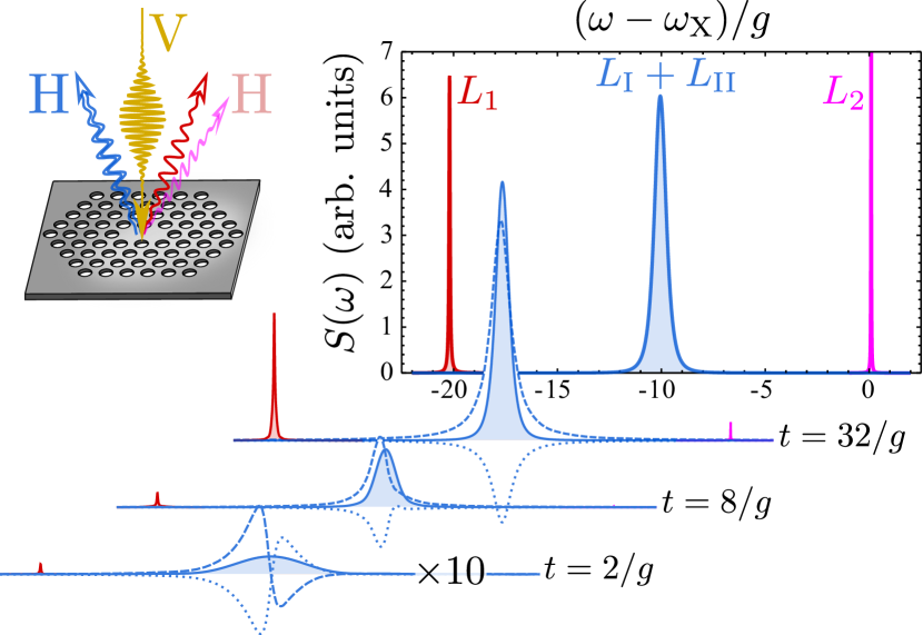
Figure 1: (color online) Cavity spectra of emission $S(t,\omega)$ at the two-photon resonance for different times (unframed) and integrated over all times (framed). They feature the 2P peak at $\omega_{a}\approx-\chi/2$ (central, blue) and the two 1P peaks at $\omega_{1}\approx-\chi$ (left, red) and $\omega_{2}\approx 0$ (right, pink). The 2P peak cannot be decomposed into two physical processes. Parameters: $\chi=20g$, $\kappa=g$, $\gamma=5\times 10^{-4}g$.

With the previous considerations, the Hamiltonian in the basis of linearly polarized states reads:

$$H=\omega_{a}a^{\dagger}a+\omega_{\mathrm{X}}(\left|\mathrm{H}\right\rangle\left\langle\mathrm{H}\right|+\left|\mathrm{V}\right\rangle\left\langle\mathrm{V}\right|)+(2\omega_{\mathrm{X}}-\chi)\left|\mathrm{B}\right\rangle\left\langle\mathrm{B}\right|\\ +g\Big{[}a^{\dagger}(\left|\mathrm{G}\right\rangle\left\langle\mathrm{H}\right|+\left|\mathrm{H}\right\rangle\left\langle\mathrm{B}\right|)+\mathrm{h.c.}\Big{]}\,,$$ (2)

where it now appears explicitly that the cavity couples only to its corresponding linear polarization ($\mathrm{H}$). Dissipation affects the bare states, i.e., in the spin-up/spin-down basis, yielding a master equation:

$$\partial_{t}\rho=i[\rho,H]+\frac{\kappa}{2}\mathcal{L}_{a}(\rho)+\frac{\gamma}{2}\sum_{i=\uparrow,\downarrow}\Big{[}\mathcal{L}_{\left|\mathrm{G}\right\rangle\left\langle i\right|}+\mathcal{L}_{\left|i\right\rangle\left\langle\mathrm{B}\right|}\Big{]}(\rho)\,,$$ (3)

where $\mathcal{L}_{c}(\rho)=2c\rho c^{\dagger}-c^{\dagger}c\rho-\rho c^{\dagger}c$, with $\kappa$ the cavity losses and $\gamma$ the exciton relaxation rates. Fig. 2 shows the configuration of levels involved in the biexciton de-excitation, that is truncated self-consistently. The coherent coupling ($g$) is represented by bidirectional (green) arrows, spontaneous decay ($\gamma$) by straight (gray) arrows and cavity decay ($\kappa$) by curly (blue) arrows, each of them linking in a reversible ($g$) or irreversible ($\gamma$, $\kappa$) way the different levels.

A one-photon resonance (1PR) is realized when the cavity is set at resonance with one of the excitonic transitions: $\left|\mathrm{B},0\right\rangle\rightarrow\left|\mathrm{H},0\right\rangle$ with frequency $\omega_{1}\approx\omega_{\mathrm{B}}-\omega_{\mathrm{X}}$ or $\left|\mathrm{H},0\right\rangle\rightarrow\left|\mathrm{G},0\right\rangle$ with frequency $\omega_{2}\approx\omega_{\mathrm{X}}$. The resonant single-photon emission is then enhanced into the cavity mode according to the conventional scenario Gérard et al. (1998), with a Purcell decay rate $\gamma_{\mathrm{P}}=4g^{2}/\kappa$. A two-photon resonance (2PR) is realized when the transition $\left|\mathrm{B},0\right\rangle\rightarrow\left|\mathrm{G},0\right\rangle$ matches energetically the emission of two cavity photons del Valle et al. (2010):

$$\omega_{a}\approx\omega_{\mathrm{X}}-\chi/2\quad\mathrm{with}\quad\chi\gg g\,,\kappa\,,\gamma\,.$$ (4)

This process also benefits from Purcell enhancement. In fact, if the decay rates $\gamma$ and $\kappa$ are small enough, two-photon Rabi oscillations between states $\left|\mathrm{B},0\right\rangle$ and $\left|\mathrm{G},2\right\rangle$ are even realized, with a characteristic frequency $g_{\mathrm{2P}}\approx 4g^{2}/(\sqrt{2}\chi)$ del Valle et al. (2010). Note that in Eq. (4), we have neglected the small Stark shifts $\sim g_{\mathrm{2P}}$, which should be taken into account to achieve maximum Rabi amplitude. In this text, to remain within experimentally achievable configurations, we consider systems in strong coupling, $g\gtrapprox\kappa$, but not so much that the two-photon oscillations actually take place, that is, we remain within the 2P weakly coupled regime, $4g_{\mathrm{2P}}\ll\kappa$. The one-photon Rabi oscillations (e.g., $\left|\mathrm{B},0\right\rangle\leftrightarrow\left|\mathrm{H},1\right\rangle$) still take place at the frequency $g$ but, as they are largely detuned, the coupling strength effectively reduces to $g_{\mathrm{1P}}\approx g/\sqrt{1+[\chi/(\gamma+\kappa)]^{2}}\approx g\kappa/\chi$ Laussy et al. (2009).

To characterize and analyze the main output of the system, shown in Fig. 1, we study the time-resolved power spectrum $S(t,\omega)\propto\Re\int_{0}^{t}dT\int_{0}^{t-T}d\tau e^{i\omega\tau}\langle a^{\dagger}(T)a(T+\tau)\rangle$ Eberly and Wódkiewicz (1977) that we compute as:

$$S(t,\omega)=\frac{1}{\pi}\sum_{\alpha\in\{1,2,\mathrm{I},\mathrm{II},\dots\}}\frac{L_{\alpha}(\gamma_{\alpha}/2)-K_{\alpha}(\omega-\omega_{\alpha})}{(\gamma_{\alpha}/2)^{2}+(\omega-\omega_{\alpha})^{2}}\,,$$ (5)

where we emphasised in the sum four dominant processes labelled $1$, $2$, $\mathrm{I}$ and $\mathrm{II}$ (results below include all processes). Each $\alpha$ corresponds to a transition in the system, characterised by its frequency ($\omega_{\alpha}$) and broadening ($\gamma_{\alpha}$) on the one hand, which allow us to identify its microscopic origin, as discussed below, and its intensity $L_{\alpha}$ and interferences with other transitions $K_{\alpha}$ Laussy et al. (2009) on the other hand. The time dependent spectra of emission can be measured experimentally with a streak camera Wiersig et al. (2009).

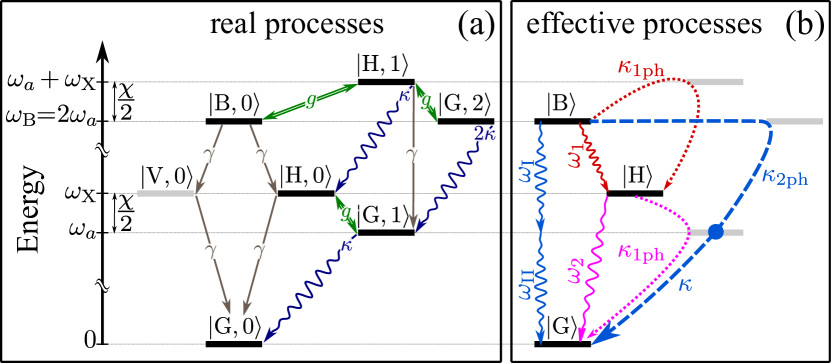
Figure 2: (color online) Level scheme of a quantum dot coupled to a cavity mode with linear polarization H at the 2PR. In (a), the microscopic configuration and in (b) the effective processes taking place in the de-excitation of the biexciton. Those involving the cavity are, on the one hand, through the emission of two real and distinguishable photons $\omega_{1}$ and $\omega_{2}$ (in dotted red and pink), and, on the other hand, through the simultaneous emission of one two-photon state at $\omega_{a}$ (in dashed blue), labelled $\omega_{\mathrm{I,II}}$.

There are two channels of de-excitation: via the cavity mode (through the annihilation of a photon $a$) or via spontaneous emission into the leaky modes (related to the four excitonic lowering operators). With the biexciton state in an empty cavity, $\left|\mathrm{B},0\right\rangle$, as the initial condition, we identify three de-excitation mechanisms of the system. We now describe them in turns.

$i$) The first decay route is a cascade of two spontaneous emissions, from $\left|B\right\rangle$ to $\left|H\right\rangle$ (or $\left|V\right\rangle$) in a first time, and then from $\left|H\right\rangle$ (or $\left|V\right\rangle$) to $\left|G\right\rangle$ in a second time, as shown in straight (gray) lines in Fig. 2(a). This decay into leaky modes is at the excitonic energies, $\omega_{1}$, $\omega_{2}$, and is a direct process with a straightforward microscopic origin as a transition between two states. Each process happens at the rate $\gamma$, so that, as far as the biexciton is concerned, its total rate of de-excitation through this channel is $2\gamma$. The effect of this channel is to reduce the efficiency of de-excitation through the cavity mode, which is the one of interest. This can be kept small by choosing a system with a small $\gamma$.

$ii$) The second decay route is another cascade of one-photon emissions, but now through the cavity mode, namely from $\left|B\right\rangle$ to $\left|G\right\rangle$ passing by $\left|H\right\rangle$. It is shown in dotted lines in Fig. 2(b). It effectively amounts to two consecutive photons into the cavity mode at the excitonic energies $\omega_{1}$ and $\omega_{2}$, also shown (with the same color code) in Fig. 2(b), but the microscopic origin is now more complex, as it involves virtual intermediate states. The first photon (1) is emitted through the process $\left|\mathrm{B},0\right\rangle\xrightarrow{\left|\mathrm{H},1\right\rangle}\left|\mathrm{H},0\right\rangle$, via the off-resonant (“virtual”) state $\left|\mathrm{H},1\right\rangle$ and the second (2), similarly through the process $\left|\mathrm{H},0\right\rangle\xrightarrow{\left|\mathrm{G},1\right\rangle}\left|\mathrm{G},0\right\rangle$. These transitions occur at the Purcell rate $\kappa_{\mathrm{1P}}\approx 4g_{\mathrm{1P}}^{2}/\kappa\approx T_{\mathrm{1P}}^{2}\kappa$, where $T_{\mathrm{1P}}=2g/\chi$ is the effective mixing parameter between states $\left|\mathrm{B},0\right\rangle$–$\left|\mathrm{H},1\right\rangle$ and $\left|\mathrm{H},0\right\rangle$–$\left|\mathrm{G},1\right\rangle$. The positions and broadenings are more precisely given by $\omega_{1}\approx-\chi-2g^{2}/\chi$, $\omega_{2}\approx 2g^{2}/\chi$ and $\gamma_{1}\approx 3\gamma$, $\gamma_{2}\approx\gamma$.

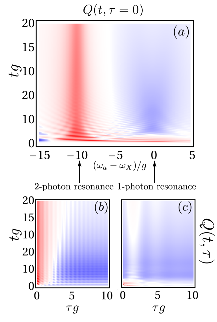
Figure 3: (color online) (a) Mandel parameter $Q(t,\tau=0)$ as a function of the cavity frequency $\omega_{a}$, for a set of typical parameters ($\chi=20g$, $\kappa=0.5g$ and $\gamma=5\times 10^{-3}g$). $Q(t,\tau)$ is shown below at the two relevant resonances, two-photon (a) and one-photon (b). There is a change in the statistics from antibunching $<0$ (1PR), colored in blue, to bunching $>0$ (2PR), colored in red.

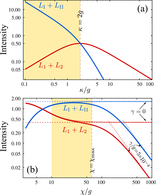
Figure 4: (color online) (a) Intensity $L_{\mathrm{I}}+L_{\mathrm{II}}$ of emission in the 2P channel (blue) and $L_{1}+L_{2}$ in the two 1P channels (red) as a function of $\kappa$ in the ideal case of nonradiative emission, $\gamma=0$ and $\chi\rightarrow\infty$. The shaded (yellow) area $\kappa<2g$ shows the region where the 2P emission dominates. (b) Same as above for $\kappa=g$ as a function of $\chi$, that must be large enough so that 1P are suppressed and small enough to maintain a high cavity emission efficiency in the realistic case of nonzero $\gamma$.

$iii$) Finally, the central event in our proposal is formed by the third channel of de-excitation of the biexciton, namely, the emission into the cavity mode of two simultaneous and indistinguishable photons with a frequency very close to that of the cavity $\omega_{\mathrm{I}}\approx\omega_{\mathrm{II}}\approx\omega_{a}$. This process is sketched by the single dashed (blue) line in Fig. 2(b), with an intermediate step marked by a point at $\left|\mathrm{G},1\right\rangle$. Effectively, this amounts to the generation of a two-photon state, represented by the two curly transitions $\omega_{\mathrm{I},\mathrm{II}}$ in Fig. 2(b). The two indices I and II strictly correspond to transitions that arise in the spectral decomposition (5), namely, $\left|\mathrm{B},0\right\rangle\xrightarrow{\left|\mathrm{G},2\right\rangle}\left|\mathrm{G},1\right\rangle$ for the first sequence of events, I, and the closing of the path, $\left|\mathrm{G},1\right\rangle\rightarrow\left|\mathrm{G},0\right\rangle$, for the second transition, II. Although we have used I and II in Fig. 2 to label the two photons for the sake of illustration, these two photons are indistinguishable and cannot be interpreted as real events taken in isolation in association with the above sequences of transitions. Indeed, each event gives rise to an unphysical spectrum (assuming negative values) and only when both processes are taken together, they interfere to sum to a physical spectrum which can be interpreted as a probability of (two-photon) detection. This decomposition of the two-photon (central) peak is shown in Fig. 1 in the time-dependent spectra, with the process I shown in a dotted line and II in dashed line. They sum to the physical (observable) peak, in solid line. Both peaks grow together in time and develop an asymmetry, one (I) being completely positive, the other (II) completely negative. None, not even the fully positive peak, can be observed in isolation. In contrast, the single-photon peaks on both sides (red and pink), are formed by single, isolated transitions, showing their real (as opposed to virtual) nature. The two-photon emission is enhanced by the Purcell rate $\kappa_{\mathrm{2P}}\approx 4g_{\mathrm{2P}}^{2}/(2\kappa)\approx T_{\mathrm{2P}}^{2}2\kappa$, where $T_{\mathrm{2P}}=g_{\mathrm{2P}}/\kappa$ is the effective mixing parameter between states $\left|\mathrm{B},0\right\rangle$-$\left|\mathrm{G},2\right\rangle$. We use $2\kappa$ because this is the decay rate of the intermediate state $\left|\mathrm{G},2\right\rangle$. One transition appears, more precisely, at $\omega_{\mathrm{I}}\approx-\chi/2+2g^{2}/\chi$ with broadening $\gamma_{\mathrm{I}}\approx\kappa+2\gamma$ (this is the sum of the decay that initial and final states suffer, $\left|\mathrm{B},0\right\rangle$ and $\left|\mathrm{G},1\right\rangle$). The other transition (II) stems from the direct process $\left|\mathrm{G},1\right\rangle\rightarrow\left|\mathrm{G},0\right\rangle$. This transition appears at $\omega_{\mathrm{II}}\approx-\chi/2-2g^{2}/\chi$ with broadening $\gamma_{\mathrm{II}}\approx\kappa$.

Another proof of the two-photon character is given by the time-dependent spectrum, Fig. 1. Whereas the single-photon events grow in succession—first the $L_{1}$ peak, that populates the state $\left|\mathrm{H}\right\rangle$, which subsequently decays to $\left|\mathrm{G}\right\rangle$, forming the $L_{2}$ peak—the two photon peak arises from the joint and simultaneous contribution of the I and II processes. In fact, one can show that at the 2PR, $L_{\mathrm{I}}+L_{\mathrm{II}}\approx 2\langle a^{\dagger 2}a^{2}\rangle$, linking directly the intensity of the peak with the two-photon emission probability. This can be brought to the experimental test by resolving the photon statistics in time, $g^{(2)}(t,\tau)=\langle a^{\dagger}(t)a^{\dagger}(t+\tau)a(t+\tau)a(t)\rangle/[n_{a}(t)n_{a}(t+\tau)]$. We use the Mandel $Q$-parameter, $Q(t,\tau)=n_{a}(t)(g^{(2)}(t,\tau)-1)$, that changes sign (negative for anticorrelations). This is shown in Fig. 3. The main panel, (a), shows a strong and sharp bunching of the emission when the cavity hits the two-photon resonance (meaning that photons come together, and in our case, in pairs), while it is antibunched in other cases (photons coming separately). What is remarkable of the two photon emission is that it is consistently bunched at all times: while the system can emit at any time, when it does, it emits the two photons together. In contrast, the 1PR emission which is antibunched as expected when the process is isolated, also has the possibility to be bunched by fortuitous joint emission of two photons. This is the case when $\omega_{a}=\omega_{2}$, the cavity is then in resonance with the lower transition, that can start only as a successor of the upper transition resulting in high probability for two photons detection, but only at very early times, since one photon is a precursor of the other one in a cascade of two otherwise distinguishable events. The proof is complete with the autocorrelation time $\tau$, shown in panels (b) and (c), further demonstrating that in the 2PR emission, the two photons arrive at zero time delay (the emission being less likely again at nonzero delay).

Now that we have demonstrated from various points of view the two-photon character of the central peak, we aim to maximise it as compared to all other de-excitation channels. There are three key parameters to enhance the 2P emission, $\kappa$, $\gamma$ and $\chi$. The case $\gamma=0$ and $\chi\rightarrow\infty$ is the ideal configuration, where all the emission goes through the cavity:

$$I_{a}=\int_{0}^{\infty}\langle a^{\dagger}a\rangle(t)\,dt=2/\kappa\,,$$ (6)

which is redistributed between the two possible decay paths as:

$$L_{1}+L_{2}\approx\frac{\kappa_{\mathrm{1P}}}{\kappa_{\mathrm{1P}}+\kappa_{\mathrm{2P}}}I_{a}\approx\frac{2}{\gamma_{\mathrm{P}}+\kappa}\,,$$ (7a)

$$L_{\mathrm{I}}+L_{\mathrm{II}}\approx\frac{\kappa_{\mathrm{2P}}}{\kappa_{\mathrm{1P}}+\kappa_{\mathrm{2P}}}I_{a}\approx\frac{2\gamma_{\mathrm{P}}/\kappa}{\gamma_{\mathrm{P}}+\kappa}\,.$$ (7b)

This is shown in Fig. 4(a), where we see that the 2P emission dominates over the 1P when $\kappa<2g$ (shaded in yellow in Fig. 4(a)), since in this case $\kappa_{\mathrm{2P}}>\kappa_{\mathrm{1P}}$. For cavities with high enough quality factor (small $\kappa$), the 2P emission is over four orders of magnitude higher than the 1P, showing that the device is extremely efficient with favourable technological parameters.

When $\gamma$ is nonzero, the situation of experimental interest, but still is the smallest parameter ($\ll\kappa,g\ll\chi$), the channel of decay it opens leads to:

$$I_{a}=\int_{0}^{\infty}n_{a}(t)\,dt=\frac{\gamma_{\mathrm{P}}(\gamma_{\mathrm{P}}+\kappa)}{\gamma\chi^{2}}\,,$$ (8)

which is now redistributed between the two cavity decay paths as an increasing function of $\chi^{-2}$:

$$L_{1}+L_{2}\approx\frac{\kappa_{\mathrm{1P}}}{\kappa_{\mathrm{1P}}+\kappa_{\mathrm{2P}}+2\gamma}I_{a}\approx\frac{\gamma_{\mathrm{P}}\kappa}{\gamma\chi^{2}}\,,$$ (9a)

$$L_{\mathrm{I}}+L_{\mathrm{II}}\approx\frac{\kappa_{\mathrm{2P}}}{\kappa_{\mathrm{1P}}+\kappa_{\mathrm{2P}}+2\gamma}I_{a}\approx\frac{\gamma_{\mathrm{P}}^{2}}{\gamma\chi^{2}}\,.$$ (9b)

This nonzero $\gamma$ case is shown in Fig. 4(b), where the ideal situation can be recovered in a region of $\chi$ bounded by above by:

$$\chi_{\mathrm{max}}=\mathrm{min}(2g\sqrt{\kappa/(2\gamma)}\,,4g^{2}/\sqrt{2\kappa\gamma})\,,$$ (10)

that follows from $2\gamma=\min(\kappa_{\mathrm{1P}},\kappa_{\mathrm{2P}})$. Above $\chi_{\mathrm{max}}$, the 2P emission still dominates over 1P emission but efficiency is spoiled, according to Eqs. (9), that are shown in dashed tilted lines.

In conclusion, we have presented a scheme where the biexciton is in two-photon resonance with a microcavity mode, as an efficient two-photon source, both in terms of the purity of the two-photon state and of its emission efficiency. The timescale for two-photon emission, that limits the repetition rate, is of the order of $\kappa_{2\mathrm{P}}^{-1}$. The quantum character of the two-photon emission is demonstrated theoretically by a detailed analysis of all the processes involved in the biexciton de-excitation, which also allows us to find analytically the optimum conditions for its realization. We have shown that the two-photons are emitted simultaneously with no delay in the autocorrelation time. Experimentally, the ultimate proof of indistinguishability can be obtained by directing the central peak to a beam-splitter, which half of the time will separate the photon pair into two ports that can then be fed in an Hong-Ou-Mandel interferometer.