Thermal diffractive corrections to Casimir energies
 

DANIEL KABAT and DIMITRA KARABALI

Department of Physics and Astronomy
Lehman College of the CUNY
Bronx, NY 10468

Abstract

We study the interplay of thermal and diffractive effects in Casimir energies. We consider plates with edges, oriented either parallel or perpendicular to each other, as well as a single plate with a slit. We compute the Casimir energy at finite temperature using a formalism in which the diffractive effects are encoded in a lower dimensional non-local field theory that lives in the gap between the plates. The formalism allows for a clean separation between direct or geometric effects and diffractive effects, and makes an analytic derivation of the temperature dependence of the free energy possible. At low temperatures, with Dirichlet boundary conditions on the plates, we find that diffractive effects make a correction to the free energy which scales as $T^{6}$ for perpendicular plates, as $T^{4}$ for slits, and as $T^{4}\log T$ for parallel plates.

1 Introduction

The Casimir effect is famous as a prototype for the influence of boundary conditions in quantum field theory. The original Casimir effect described the interaction between two infinite parallel conducting plates due to vacuum fluctuations of the electromagnetic field [1]. Since that pioneering work many variants of the effect have been studied. For recent reviews see [2].

It is interesting to ask how the Casimir energy is modified when the plates have boundaries, either apertures or edges. That is, it is interesting to ask how diffractive effects correct the Casimir energy. We studied this in [3] using a formalism which we will review below. An advantage of our formalism is that it allows for a clean separation between direct or geometrical effects associated with the plates, and diffractive effects associated with the plate boundaries. In [3] we considered several geometries: two perpendicular plates separated by a gap, a single plate with a slit in it, and two parallel plates, one of which is semi-infinite. For other approaches to analyzing the Casimir energy in such geometries see [4, 5, 6].

In the present paper we extend our results to finite temperature. One of our motivations is to obtain an analytic understanding of the non-trivial correlation between geometry and temperature found in [7, 8] using worldline Monte Carlo techniques. Although the high temperature limit of the Casimir energy obeys a well understood, linear dependence on temperature, the low temperature limit is much more subtle and depends crucially on the global configuration of the plates.

By way of outline, in section 2 we set up the formalism at finite temperature and collect some useful preliminary results. We study the behavior at low temperature in section 3, with perpendicular plates in section 3.1, slits in section 3.2, and parallel plates in section 3.3. We conclude in section 4. Appendix A collects some useful results on the partition function of an ideal gas.

2 An effective action for edge effects

We consider a free massless scalar field in four dimensions, with Dirichlet boundary conditions imposed on an arrangement of plates. The basic plate geometry we will consider is shown in Fig. 1. Besides the two dimensions shown in the figure, the full geometry also has a periodic spatial dimension of size $L_{z}$ and a periodic Euclidean time dimension of size $\beta$. For simplicity we will always have in mind the limit $L_{x},\,L_{z}\rightarrow\infty$, but as we are interested in finite temperature we will keep $\beta$ fixed.

Starting from the geometry in Fig. 1, but restricting to field configurations which are odd under $x\rightarrow-x$, is equivalent to imposing a Dirichlet boundary condition at $x=0$. That is, it corresponds to the effective arrangement of plates shown in Fig. 2.

Figure 1: A two-dimensional slice through the geometry. Dirichlet boundary conditions are imposed on the solid lines. The gap between the plates (where the non-local field theory lives) is indicated by a dashed line. The four-dimensional geometry also has a periodic spatial dimension of size $L_{z}$ out of the page and a periodic Euclidean time dimension of size $\beta$.

Figure 2: The effective plate geometry for odd-parity modes.

For reasons discussed below, we will focus on three special cases:

• a single plate with a slit, corresponding to $b_{1},\,b_{2}\rightarrow\infty$, $w=2a$ fixed in Fig. 1;

• perpendicular plates, corresponding to $b_{1},\,b_{2}\rightarrow\infty$, $a$ fixed in Fig. 2;

• parallel plates, corresponding to $a,\,b_{1}\rightarrow\infty$, $b=b_{2}$ fixed in Fig. 2.

The basic strategy, developed in [3], is to do the Euclidean path integral in stages. We first fix the value of the field in the gap between the plates, setting $\phi=\phi_{0}$ on the dashed line indicated in the figures, and subsequently integrate over $\phi_{0}$. In other words we write the Euclidean partition function as

$$Z=\int{\cal D}\phi_{0}\,\int_{\raisebox{-5.0pt}{$\phi|_{\rm gap}=\phi_{0}$}}{\cal D}\phi\,\,\,\,e^{-\int d^{4}x\,{1\over 2}\partial\phi\cdot\partial\phi}$$ (1)

By integrating out the scalar field in the bulk regions (top and bottom) we obtain a non-local effective action for $\phi_{0}$. To perform the bulk path integral we set $\phi=\phi_{\rm cl}+\delta\phi$ where $\delta\phi$ vanishes on all boundaries (including the gap), and $\Box\phi_{\rm cl}=0$ subject to the boundary conditions

$$\phi_{\rm cl}\rightarrow\left\{\begin{array}[]{ll}\phi_{0}&\hbox{\rm in gap}\\ 0&\hbox{\rm elsewhere on boundary}\end{array}\right.$$ (2)

The action for $\delta\phi$ separates into top and bottom contributions leading to

$$Z = \det{}^{-1/2}(-\Box_{\rm top})\det{}^{-1/2}(-\Box_{\rm bottom})\,\int{\cal D}\phi_{0}\,e^{-S_{0}}$$

$$S_{0} = \int d^{4}x\,{1\over 2}\partial\phi_{\rm cl}\cdot\partial\phi_{\rm cl}$$ (3)

where $\Box_{\rm top},\,\Box_{\rm bottom}$ are the corresponding Laplacians. Given the boundary conditions on $\delta\phi$, the bulk determinants are to be evaluated with Dirichlet boundary conditions everywhere, including the part of the boundary which corresponds to the gap.

$\phi_{\rm cl}$ can be written in terms of $\phi_{0}$ and the Green’s functions $G_{\rm top}$ and $G_{\rm bottom}$. These obey Dirichlet boundary conditions and satisfy $\Box G(x|x^{\prime})=\delta^{4}(x-x^{\prime})$ in the bulk regions.

$$\phi_{\rm cl}(x)=\left\{\begin{array}[]{ll}\int d^{3}x^{\prime}\,\phi_{0}(x^{\prime})\,n\cdot\partial^{\prime}G_{\rm top}(x|x^{\prime})&\hbox{\rm on top}\\[8.0pt] \int d^{3}x^{\prime}\,\phi_{0}(x^{\prime})\,n\cdot\partial^{\prime}G_{\rm bottom}(x|x^{\prime})&\hbox{\rm on bottom}\end{array}\right.$$ (4)

Here $n$ is an outward-pointing unit normal vector. Integrating by parts, the classical action in (2) becomes a surface term,

$$S_{0}=\int d^{3}x\,\int d^{3}x^{\prime}~{}{1\over 2}\phi_{0}(x)\,(M_{\rm top}(x|x^{\prime})+M_{\rm bottom}(x|x^{\prime}))~{}\phi_{0}(x^{\prime})$$ (5)

$$M(x|x^{\prime})=n\cdot\partial\,n\cdot\partial^{\prime}G(x|x^{\prime})$$ (6)

The operator $M(x|x^{\prime})$ is defined on the boundary between the bulk regions including the gap.

The bulk determinants in (2) capture the Casimir energy that would be present if there was no gap in the middle plate. Corrections to this are given by a non-local field theory that lives on the gap separating the two regions. We can write a mode expansion for the fields $\phi_{0}$ as $\phi_{0}({x})=\sum_{\alpha}c_{\alpha}u_{\alpha}({x})$ where $\left\{u_{\alpha}({x})\right\}$ constitute a complete set of modes for functions which are nonzero in the gap with the boundary condition that $u_{\alpha}({x})\rightarrow 0$ as one approaches the edges. Integrating over $c_{\alpha}$ leads to a representation of the four-dimensional partition function

$$Z_{\rm 4d}=\det{}^{-1/2}\big{(}-\Box_{\rm top}\big{)}\,\det{}^{-1/2}\big{(}-\Box_{\rm bottom}\big{)}\,\det{}^{-1/2}\big{(}{\cal O}_{\rm top}+{\cal O}_{\rm bottom}\big{)}$$ (7)

where

$${\cal O}_{\alpha\beta}=\int_{\rm gap}d^{3}{x}~{}d^{3}{x^{\prime}}~{}u_{\alpha}(x)M(x|x^{\prime})~{}u_{\beta}(x^{\prime})$$ (8)

Because the mode functions $u_{a}(x)$ vanish outside the gap, the operators ${\cal O}$ are essentially the projected versions of $M(x|x^{\prime})$ onto the gap, ${\cal O}=PMP$, where $P$ is a projection operator onto functions with support in the gap. That is

$$Pf(x)=\left\{\begin{array}[]{ll}f(x)&\hbox{\rm if $x\in{\rm gap}$}\\ 0&\hbox{\rm otherwise}\end{array}\right.$$

The explicit form of the operator $M(x|x^{\prime})$ and its projected version ${\cal O}$ depends, in general, on the arrangement of plates and gaps. For the geometries shown in Figs. 1 and 2, the non-local operators which appear in the effective action for $\phi_{0}$ are [3]

$${\cal O}_{\rm top}=P{\sqrt{-\nabla^{2}}\over\tanh\big{(}b_{1}\sqrt{-\nabla^{2}}\big{)}}\,P$$ (9)

$${\cal O}_{\rm bottom}=P{\sqrt{-\nabla^{2}}\over\tanh\big{(}b_{2}\sqrt{-\nabla^{2}}\big{)}}\,P$$

Here $\nabla^{2}$ is the 3-dimensional Laplace operator defined on the middle plate (including the gap) and $P$ is a projection operator onto functions with support in the gap.

At this stage it is convenient to make a Kaluza-Klein decomposition along the two extra periodic directions. This leads to a representation of the four dimensional partition function in terms of a momentum integral and a sum over Matsubara frequencies.

$$\log Z_{\rm 4d}=L_{z}\int{dk\over 2\pi}\sum_{l=-\infty}^{\infty}\log Z_{\rm 2d}\Big{(}\mu=\sqrt{k^{2}+(2\pi l/\beta)^{2}}\Big{)}$$ (10)

Here $Z_{\rm 2d}(\mu)$ is the two-dimensional partition function for a scalar field of mass $\mu$ in the geometry shown in Fig. 1 or 2.

The representation (10) makes it apparent that in the high-temperature limit ($\beta\rightarrow 0$) only the $l=0$ mode contributes and the problem reduces to a partition function in three dimensions. Thus in the high-temperature limit the partition function is independent of $T$, and the free energy is linear in $T$, independent of the geometry. The behavior at low temperatures is more subtle and will be considered in section 3.

For the geometry of Fig. 1, a complete set of odd- and even-parity functions which vanish for $|x|\geqslant a$ are

$$u^{\rm odd}_{m}=\left\{\begin{array}[]{cl}(-1)^{m}{1\over\sqrt{a}}\sin\left(m\pi x/a\right)&\hbox{\rm for $-a\leqslant x\leqslant a$}\qquad m=1,2,3,\ldots\\ 0&\hbox{\rm otherwise}\end{array}\right.$$ (13)

$$u^{\rm even}_{p}=\left\{\begin{array}[]{cl}(-1)^{p+{1\over 2}}{1\over\sqrt{a}}\cos\left(p\pi x/a\right)&\hbox{\rm for $-a\leqslant x\leqslant a$}\qquad p={1\over 2},{3\over 2},{5\over 2},\ldots\\ 0&\hbox{\rm otherwise}\end{array}\right.$$ (16)

Matrix elements of the operators (9) can be evaluated in this basis as in (8). For the operator (denoting $d_{x}={d\over dx}$)

$${\cal O}=P{\sqrt{-d_{x}^{2}+\mu^{2}}\over\tanh\big{(}b\sqrt{-d_{x}^{2}+\mu^{2}}\big{)}}\,P$$

we have the matrix elements

$${\cal O}^{\rm odd}_{mn} = {2a\over\pi}\int_{-\infty}^{\infty}dk\,\sin^{2}(ka)\,M(k)\,{m\pi\over k^{2}a^{2}-m^{2}\pi^{2}}\,{n\pi\over k^{2}a^{2}-n^{2}\pi^{2}}$$ (17)

$${\cal O}^{\rm even}_{pq} = {2a\over\pi}\int_{-\infty}^{\infty}dk\,\cos^{2}(ka)\,M(k)\,{p\pi\over k^{2}a^{2}-p^{2}\pi^{2}}\,{q\pi\over k^{2}a^{2}-q^{2}\pi^{2}}$$ (18)

where $m,n=1,2,\cdots$, $p,q=1/2,3/2,\cdots$, and $M(k)={\sqrt{k^{2}+\mu^{2}}\over\tanh\big{(}b\sqrt{k^{2}+\mu^{2}}\big{)}}$ has the useful representation

$$M(k)={1\over b}+{2\over b}\sum_{j=1}^{\infty}{k^{2}+\mu^{2}\over k^{2}+\mu^{2}+{j^{2}\pi^{2}\over b^{2}}}\,.$$

As discussed in [3], by contour deformation the matrix elements can be decomposed into “direct” and “diffractive” contributions. For the odd matrix elements

$${\cal O}^{\rm odd}_{mn}={\cal O}_{mn}^{\rm direct}+{\cal O}_{mn}^{\rm diffractive}$$ (19)

$${\cal O}_{mn}^{\rm direct}={\sqrt{(m\pi/{a})^{2}+\mu^{2}}\over\tanh\big{(}b\sqrt{(m\pi/{a})^{2}+\mu^{2}}\big{)}}\,\delta_{mn}$$ (20)

$${\cal O}_{mn}^{\rm diffractive}=-2ab^{2}\sum_{j=1}^{\infty}\left(1-\exp\Big{(}-{2a\over b}\sqrt{j^{2}\pi^{2}+\mu^{2}b^{2}}\Big{)}\right){j^{2}\pi^{2}\over\sqrt{j^{2}\pi^{2}+\mu^{2}b^{2}}}$$

$$\qquad\qquad\qquad{m\pi\over(m\pi b)^{2}+(j\pi a)^{2}+(\mu ab)^{2}}\,\,{n\pi\over(n\pi b)^{2}+(j\pi a)^{2}+(\mu ab)^{2}}$$ (21)

Likewise for the even matrix elements

$${\cal O}^{\rm even}_{pq}={\cal O}_{pq}^{\rm direct}+{\cal O}_{pq}^{\rm diffractive}$$ (22)

$${\cal O}_{pq}^{\rm direct}={\sqrt{(p\pi/{a})^{2}+\mu^{2}}\over\tanh\big{(}b\sqrt{(p\pi/{a})^{2}+\mu^{2}}\big{)}}\,\delta_{pq}$$ (23)

$${\cal O}_{pq}^{\rm diffractive}=-2ab^{2}\sum_{j=1}^{\infty}\left(1+\exp\Big{(}-{2a\over b}\sqrt{j^{2}\pi^{2}+\mu^{2}b^{2}}\Big{)}\right){j^{2}\pi^{2}\over\sqrt{j^{2}\pi^{2}+\mu^{2}b^{2}}}$$

$$\qquad\qquad\qquad{p\pi\over(p\pi b)^{2}+(j\pi a)^{2}+(\mu ab)^{2}}\,\,{q\pi\over(q\pi b)^{2}+(j\pi a)^{2}+(\mu ab)^{2}}$$ (24)

(Aside from the allowed values of the indices, the only difference between odd and even parity is the sign in front of the exponential in the diffractive term.) Finally, to study the perpendicular plate geometry of Fig. 2, we only need to keep the odd-parity modes (13). Thus the matrix elements for perpendicular plates are exactly those given in (19) – (21).

The direct contribution takes into account wave propagation directly across the gap. Note that it is diagonal in the basis we are using. Mathematically ${\cal O}^{\rm direct}$ is simply the operator ${\sqrt{-d_{x}^{2}+\mu^{2}}\over\tanh\big{(}b\sqrt{-d_{x}^{2}+\mu^{2}}\big{)}}$, defined with Dirichlet boundary conditions at $x=-a$ and $x=a$. Corrections to this, which incorporate diffraction of waves through the gap, are encoded in ${\cal O}^{\rm diffractive}$.

The approach developed in [3] was to treat diffraction as a small perturbation. Taking the log of (7) and expanding in powers of ${\cal O}^{\rm diffractive}$, the 4d free energy naturally decomposes into bulk, direct and diffractive contributions.

$$-\log Z_{\rm bulk} = {1\over 2}{\rm Tr}\log\big{(}-\Box_{\rm top}\big{)}+{1\over 2}{\rm Tr}\log\big{(}-\Box_{\rm bottom}\big{)}$$ (25)

$$-\log Z_{\rm direct} = {1\over 2}{\rm Tr}\log\big{(}{\cal O}_{\rm top}^{\rm direct}+{\cal O}_{\rm bottom}^{\rm direct}\big{)}$$ (26)

$$-\log Z_{\rm diffractive} = {1\over 2}{\rm Tr}\left[\left({\cal O}^{\rm direct}\right)^{-1}{\cal O}^{\rm diffractive}\right]$$

$$-{1\over 4}{\rm Tr}\left[\left({\cal O}^{\rm direct}\right)^{-1}{\cal O}^{\rm diffractive}\left({\cal O}^{\rm direct}\right)^{-1}{\cal O}^{\rm diffractive}\right]$$

$$+\cdots$$

$$= -\log Z^{(1)}_{\rm diffractive}-\log Z^{(2)}_{\rm diffractive}+\cdots$$ (28)

where in (2)

$${\cal O}^{\rm direct}={\cal O}_{\rm top}^{\rm direct}+{\cal O}_{\rm bottom}^{\rm direct}$$

$${\cal O}^{\rm diffractive}={\cal O}_{\rm top}^{\rm diffractive}+{\cal O}_{\rm bottom}^{\rm diffractive}$$ (29)

The bulk and direct contributions (25), (26) are basically Bose partition functions and can be calculated analytically. The relevant calculations are summarized in appendix A. Our main interest in the next section will be diffractive effects.

3 Thermal free energy: low temperature limit

In this section we study the behavior of the partition function (10) at low temperatures. Applying Poisson resummation to (10) gives

$$\log Z_{\rm 4d}=\sum_{l=-\infty}^{\infty}\beta L_{z}\int{dk\over 2\pi}{d\omega\over 2\pi}e^{-i\beta\omega l}\log Z_{\rm 2d}\big{(}\mu=\sqrt{k^{2}+\omega^{2}}\big{)}$$ (30)

The $l=0$ term is proportional to $\beta$. It gives the Casimir energy at zero temperature that was studied in [3]. Thermal corrections to this are given by

$$\log Z_{\rm 4d,T}={\beta L_{z}\over\pi}\sum_{l=1}^{\infty}\int_{0}^{\infty}\mu d\mu J_{0}(\beta l\mu)\log Z_{\rm 2d}(\mu)$$ (31)

where we set $\omega=\mu\cos\theta$, $k=\mu\sin\theta$ and integrated over $\theta$.

It is clear that the behavior of (31) at low temperature, $\beta\rightarrow\infty$, is related to the behavior of $\log Z_{\rm 2d}$ as $\mu\rightarrow 0$. For instance if $\log Z_{\rm 2d}(\mu)$ is analytic as a function of $\mu^{2}$ along the positive real $\mu^{2}$ axis then the 4d free energy will vanish exponentially at low temperature. On the other hand, assuming that $\log Z_{\rm 2d}$ does not diverge for large $\mu$, we can use

$$\int_{0}^{\infty}dx\,J_{0}(\beta x)x^{\nu-1}=-{2^{\nu}\Gamma(\nu/2)\over\nu\Gamma(-\nu/2)}\,{1\over\beta^{\nu}}$$ (32)

So power-law behavior of the 2d free energy as $\mu\rightarrow 0$, $\log Z_{\rm 2d}\sim\mu^{\nu-2}$, will in general lead to power-law behavior of the 4d free energy at low temperature, $\log Z_{\rm 4d}\sim T^{\nu}$. (In accord with our analyticity arguments, the coefficient of $T^{\nu}$ vanishes for $\nu=2,4,6,\ldots$)

For future use it is convenient to define $f(\nu)=-{2^{\nu}\Gamma(\nu/2)\over\nu\Gamma(-\nu/2)}$. Differentiating (32) with respect to $\nu$ gives the useful identities

$$\int_{0}^{\infty}dx\,J_{0}(\beta x)x^{\nu-1}=f(\nu)\,{1\over\beta^{\nu}}$$ (33)

$$\int_{0}^{\infty}dx\,J_{0}(\beta x)x^{\nu-1}\log x=-f(\nu)\,{1\over\beta^{\nu}}\log\beta+f^{\prime}(\nu){1\over\beta^{\nu}}$$ (34)

$$\int_{0}^{\infty}dx\,J_{0}(\beta x)x^{\nu-1}(\log x)^{2}=f(\nu)\,{1\over\beta^{\nu}}(\log\beta)^{2}-2f^{\prime}(\nu){1\over\beta^{\nu}}\log\beta+f^{\prime\prime}(\nu){1\over\beta^{\nu}}\qquad$$ (35)

We will evaluate thermal contributions to the free energy using the representation (31). If the geometric parameters $a,b_{1},b_{2}$ are held fixed then, from (20) – (24), all matrix elements are analytic in $\mu^{2}$ about $\mu=0$. The 2d partition function inherits this analyticity, which means that at low temperatures the 4d free energy is exponentially suppressed. As a result, we proceed to study three special cases which have interesting power-law behavior at low temperature:

• perpendicular plates,

• a slit geometry,

• parallel plates.

3.1 Perpendicular plates

In this section we study the low temperature behavior of the free energy for perpendicular plates. The geometry of interest is shown in Fig. 3. However to regulate IR divergences we actually work with the geometry of Fig. 4 in the limit $b,\,L_{x}\rightarrow\infty$.

Figure 3: Perpendicular plates. The dashed line indicates the gap between the plates. There is also a periodic spatial dimension of size $L_{z}\rightarrow\infty$ pointing out of the page and a periodic Euclidean time dimension of size $\beta$.

Figure 4: Regulated geometry for perpendicular plates.

There are three contributions to the thermal free energy.

Bulk contribution
The bulk contribution (25) from the regions above and below the middle plate is that of an ideal Bose gas. This is worked out in (A). Including surface contributions associated with the Dirichlet boundary conditions, the free energy is

$$F^{\rm bulk}_{\rm top}=F^{\rm bulk}_{\rm bottom}=-{\zeta(4)\over\pi^{2}}bL_{x}L_{z}T^{4}+{\zeta(3)\over 4\pi}(L_{x}+b)L_{z}T^{3}-{\zeta(2)\over 4\pi}L_{z}T^{2}$$ (36)

To isolate the thermal Casimir energy associated with the gap in the middle plate we proceed as follows. First we subtract the free energy of a “big box” of volume $2b\times L_{x}\times L_{z}$ without any middle plate. This is given by

$$F_{\rm box}=-{\zeta(4)\over\pi^{2}}2bL_{x}L_{z}T^{4}+{\zeta(3)\over 4\pi}(L_{x}+2b)L_{z}T^{3}-{\zeta(2)\over 4\pi}L_{z}T^{2}$$ (37)

Next we subtract the thermal self-energy of the middle plate itself, as well as the thermal self-energy associated with the “$\dashv\,$” shaped junction on the right side of Fig. 4. These are given by

$$F_{\rm self}={\zeta(3)\over 4\pi}(L_{x}-a)L_{z}T^{3}-{\zeta(2)\over 8\pi}L_{z}T^{2}$$ (38)

Thus the bulk contribution to the thermal Casimir free energy for perpendicular plates is

$$F^{\rm bulk}_{\perp,T}=F^{\rm bulk}_{\rm top}+F^{\rm bulk}_{\rm bottom}-F_{\rm box}-F_{\rm self}={\zeta(3)\over 4\pi}L_{z}aT^{3}-{\zeta(2)\over 8\pi}L_{z}T^{2}$$ (39)

Eq. (39) provides the leading low temperature behavior of the Casimir energy and it agrees with the results on the thermal Casimir force found in [7, 8].

Direct contribution
To evaluate the direct contribution to the free energy (26), note from (20) that as $b\rightarrow\infty$ the direct matrix elements are given by

$${\cal O}_{mn}^{\rm direct}=\sqrt{(m\pi/a)^{2}+\mu^{2}}\,\delta_{mn}$$ (40)

Thus the direct contribution to the free energy can be identified with half the free energy of an ideal gas in $2+1$ dimensions, where the gas occupies the region corresponding to the gap. This free energy is worked out in appendix A equation (109). We find that

$$F^{\rm direct}_{\perp,T}=-{L_{z}T\over{2a}}\sum_{m,n=1}^{\infty}{{m}\over{n}}K_{1}({{mn\pi}/{aT}})$$ (41)

At low temperatures, $aT<<1$, the direct contribution to the thermal free energy is exponentially suppressed since the thermal wavelength does not fit in the gap.

First diffractive contribution
To evaluate the diffractive contribution to the free energy (2) we need to study the operator ${\cal O}^{\rm diffractive}_{\perp}$. As $b\rightarrow\infty$ we can replace the sum in (21) with an integral to obtain

$${\cal O}_{\perp,mn}^{\rm diffractive}=-{2\over\pi a^{3}}\int_{0}^{\infty}dk\,\left(1-e^{-2a\sqrt{k^{2}+\mu^{2}}}\right){k^{2}\over\sqrt{k^{2}+\mu^{2}}}\,\,{m\pi\over(m\pi/a)^{2}+k^{2}+\mu^{2}}\,\,{n\pi\over(n\pi/a)^{2}+k^{2}+\mu^{2}}$$ (42)

Using (40) and (42) in (2), at first order in perturbation theory the diffractive contribution to the 2d partition function is, with $x=a\sqrt{k^{2}+\mu^{2}}$,

$$-\log Z_{\rm 2d}^{\rm diffractive}=-{1\over\pi}\sum_{n=1}^{\infty}{n^{2}\pi^{2}\over\sqrt{n^{2}\pi^{2}+\mu^{2}a^{2}}}\,\int_{\mu a}^{\infty}dx\sqrt{x^{2}-\mu^{2}a^{2}}\,\big{(}1-e^{-2x}\big{)}{1\over\big{(}x^{2}+n^{2}\pi^{2}\big{)}^{2}}$$ (43)

At this point we need to determine the non-analytic behavior as $\mu\rightarrow 0$ of the integral

$$I=\int_{\mu a}^{\infty}dx\sqrt{x^{2}-\mu^{2}a^{2}}\,\left[\big{(}1-e^{-2x}\big{)}{1\over\big{(}x^{2}+n^{2}\pi^{2}\big{)}^{2}}\right]$$ (44)

To obtain this we split the region of integration in two, introducing an intermediate scale $x_{0}$ with $\mu a\ll x_{0}\ll 1$. We evaluate the integral (44) in the region $\mu a<x<x_{0}$ by expanding the quantity in square brackets in powers of $x$ and integrating term-by-term. Only even powers of $x$ in this expansion give contributions which are non-analytic in $\mu^{2}$. Similarly, we evaluate the integral in the region $x_{0}<x<\infty$ by expanding $\sqrt{x^{2}-\mu^{2}a^{2}}$ in powers of $\mu^{2}$ and integrating term-by-term. This of course gives a contribution which is analytic in $\mu^{2}$. One can check that, order by order, the final result does not depend on the intermediate scale $x_{0}$. This procedure gives

$$I= -{1\over 4n^{4}\pi^{4}}(\mu a)^{4}\log\mu a+\left({1\over 4n^{6}\pi^{6}}-{1\over 24n^{4}\pi^{4}}\right)(\mu a)^{6}\log\mu a+\cdots$$ (45)

$$+\,(\hbox{\rm terms analytic in $\mu^{2}$})$$

Substituting this in (43) and evaluating the sum on $n$ gives the non-analytic behavior of the 2d partition function.

$$-\log Z_{2d}^{\rm diffractive}={\zeta(3)\over 4\pi^{4}}(\mu a)^{4}\log\mu a+\left({\zeta(3)\over 24\pi^{4}}-{3\zeta(5)\over 8\pi^{6}}\right)(\mu a)^{6}\log\mu a+\cdots$$ (46)

From (31) the leading low temperature behavior of the 4d thermal free energy is then

$$F_{\perp,T}^{\rm diffractive}={L_{z}\zeta(3)\over 4\pi^{5}a^{2}}\sum_{l=1}^{\infty}\int_{0}^{\infty}d(\mu a)J_{0}(\beta l\mu)(\mu a)^{5}\log(\mu a)$$

This integral is evaluated using (34). In the case at hand $f(6)=0$ and $f^{\prime}(6)=-64$. Doing the sum on $l$, the first diffractive correction to the free energy is

$$F_{\perp,T}^{(1)\rm diffractive}=-{16\pi\zeta(3)\over 945}L_{z}a^{4}T^{6}+{\cal O}(T^{8})$$ (47)

Higher diffractive contributions
In [3] we studied higher order terms in the expansion (28). We found that the $n^{th}$ order diffractive contribution to $-\log Z_{\rm 2d}$ for perpendicular plates is of the form

$$-\log Z_{\rm 2d}^{(n){\rm diffractive}}=-{2^{n-1}\over n}\int_{1}^{\infty}\prod^{n}_{i=1}dy_{i}\sqrt{y_{i}^{2}-1}\left(1-e^{-2\mu ay_{i}}\right)T(\mu a)\ast T(\mu a)\ast\cdots\ast T(\mu a)$$ (48)

where

$$T\ast T\ast\cdots\ast T=T(\mu a,y_{1},y_{2})T(\mu a,y_{2},y_{3})\cdots T(\mu a,y_{n},y_{1})$$

and

$$T(\mu a,y,z)={\mu^{2}a^{2}\over\pi}\sum_{r=1,2,\cdots}{r^{2}\pi^{2}\over\sqrt{r^{2}\pi^{2}+\mu^{2}a^{2}}~{}(r^{2}\pi^{2}+\mu^{2}a^{2}y^{2})~{}(r^{2}\pi^{2}+\mu^{2}a^{2}z^{2})}$$ (49)

Using the change of variables $x_{i}=\mu ay_{i}$ and analyzing each of the $x_{i}$ integrals as outlined below (44), we find that the small $\mu$ behavior of the 2d partition function is characterized by analytic and non-analytic terms of the form

$$-\log Z_{\rm 2d}^{(n){\rm diffractive}} = \sum_{r=1}^{n}\sum_{l=0}^{\infty}A_{rl}(\mu a)^{4r+2l}(\log\mu a)^{r}$$

$$+ (\hbox{\rm terms analytic in $\mu^{2}$})$$

The second order diffractive contribution to the $(\mu a)^{4}\log({\mu a})$ term is $0.00031~{}(\mu a)^{4}\log\mu a$. This is a $10\%$ correction compared to the first order term ${\zeta(3)\over 4\pi^{4}}(\mu a)^{4}\log\mu a$ in (46). Higher order effects are much smaller.

Logarithms of the temperature arise at higher orders in perturbation theory. Indeed, using relations similar to (35), but applied to higher $\log$-terms, we find that the $n^{th}$ order diffractive term in the perturbative expansion contributes to the thermal free energy new log-terms of the form $T^{4n+2+2l}(\log T)^{n-1},~{}~{}l=0,1,\cdots$. The first $\log T$ term is of order $T^{10}\log T$ and can be neglected at low $T$.

Summary
Collecting our results, the low temperature behavior of the free energy for perpendicular plates, up to first order in diffractive effects, is

$$F_{\perp,T}=-{\zeta(2)\over 8\pi}L_{z}T^{2}+{\zeta(3)\over 4\pi}L_{z}aT^{3}-{16\pi\zeta(3)\over 945}L_{z}a^{4}T^{6}+{\cal O}(T^{8})$$ (51)

The two leading terms come from the bulk determinants. They have a simple physical interpretation. At low temperatures ($aT\ll 1$) the thermal wavelength is larger than the size of the gap. As a result the field does not see the gap and behaves as though a Dirichlet boundary condition had been imposed there. So the thermal renormalization of the tension associated with a Dirichlet boundary and a “$\,\vdash$” shaped junction also applies to the gap. This effect can be thought of as an excluded area effect, and is responsible for the leading low temperature behavior of the Casimir energy. Diffractive effects are subleading, beginning at ${\cal O}(T^{6})$, while the direct contribution from the theory in the gap is exponentially suppressed.

3.2 Slit geometry

In this section we study the low temperature behavior of the free energy for a slit of width $w=2a$. The corresponding geometry is shown in Fig. 5.

Figure 5: Slit geometry. The dashed line indicates the gap between the plates. There is also a periodic spatial dimension of size $L_{z}\rightarrow\infty$ pointing out of the page and a periodic Euclidean time dimension of size $\beta$.

There are again three contributions to the thermal free energy.

Bulk contribution
The bulk contribution for the slit is very similar to the one found for the perpendicular plates. The contribution from the regions above and below the middle plate is that of an ideal Bose gas as in (36). In isolating the thermal Casimir energy associated with the slit, we subtract the free energy of the “big box” as given in (37) and the self energy of the middle plate which is

$$F_{\rm self}={\zeta(3)\over 4\pi}(L_{x}-w)L_{z}T^{3}-{\zeta(2)\over 4\pi}L_{z}T^{2}$$ (52)

The final bulk contribution to the free energy is

$$F^{\rm bulk}_{\perp,T}=F^{\rm bulk}_{\rm top}+F^{\rm bulk}_{\rm bottom}-F_{\rm box}-F_{\rm self}={\zeta(3)\over 4\pi}L_{z}wT^{3}$$ (53)

Direct contribution
To evaluate the direct contribution to the free energy (26), note from (20) and (23), that as $b\rightarrow\infty$ the direct matrix elements are given by

$${\cal O}_{ll^{\prime}}^{\rm direct}=\sqrt{(l\pi/w)^{2}+\mu^{2}}\,\delta_{ll^{\prime}}$$ (54)

where both odd (20) and even terms (23) have been included. The direct contribution to the free energy is given by (41), where $a\rightarrow w$, and it is exponentially suppressed as expected.

First diffractive contribution
To evaluate the diffractive contribution to the free energy (2) we need to study the operator ${\cal O}^{\rm diffractive}_{\rm slit}$. As $b\rightarrow\infty$ we can replace the sum in (21) and (24) with an integral to obtain

$${\cal O}_{{\rm slit},ll^{\prime}}^{\rm diffractive}=-{4\over\pi w^{3}}\int_{0}^{\infty}dk\,\left[1-(-1)^{l}e^{-w\sqrt{k^{2}+\mu^{2}}}\right]{k^{2}\over\sqrt{k^{2}+\mu^{2}}}\,\,{l\pi\over(l\pi/w)^{2}+k^{2}+\mu^{2}}\,\,{l^{\prime}\pi\over(l^{\prime}\pi/w)^{2}+k^{2}+\mu^{2}}$$ (55)

Using (54) and (55) in (2), at first order in perturbation theory, the diffractive contribution to the 2d partition function is

$$-\log Z_{\rm 2d}^{\rm diffractive}=-\log Z_{\rm 2d}^{\rm odd,diffractive}-\log Z_{\rm 2d}^{\rm even,diffractive}$$

$$= -{4\over{\pi w^{3}}}\sum_{l=1}^{\infty}{l^{2}\pi^{2}\over\sqrt{(l\pi/w)^{2}+\mu^{2}}}\int_{0}^{\infty}dk\,\left[1-(-1)^{l}e^{-w\sqrt{k^{2}+\mu^{2}}}\right]{k^{2}\over\sqrt{k^{2}+\mu^{2}}}\,{1\over{[(l\pi/w)^{2}+k^{2}+\mu^{2}]^{2}}}$$

where $-\log Z_{\rm 2d}^{\rm odd,diffractive}$ accounts for the contribution of the odd modes $l=2m$ and $-\log Z_{\rm 2d}^{\rm even,diffractive}$ accounts for the contribution of the even modes $l=2p+1$. Using $w=2a$ and changing variables to $x=a\sqrt{k^{2}+\mu^{2}}$ we find that $-\log Z_{\rm 2d}^{\rm odd,diffractive}$ is identical to the expression (43) for the perpendicular plates. As we saw in section 3.1, this produces a diffractive correction to the thermal free energy of order $T^{6}$ at low temperatures, namely

$$F_{\rm slit,T}^{(1)\rm odd,diffractive}=-{{16\pi\zeta(3)}\over{945}}L_{z}a^{4}T^{6}+{\cal O}(T^{8})$$ (57)

Next we focus on the contribution of the even modes.

$$-\log Z_{\rm 2d}^{\rm even,diffractive}=-{1\over\pi}\sum_{p=1/2,3/2,\cdots}{p^{2}\pi^{2}\over\sqrt{p^{2}\pi^{2}+\mu^{2}a^{2}}}\,\int_{\mu a}^{\infty}dx\sqrt{x^{2}-\mu^{2}a^{2}}\,\big{(}1+e^{-2x}\big{)}{1\over\big{(}x^{2}+p^{2}\pi^{2}\big{)}^{2}}$$ (58)

At this point we need to determine the non-analytic behavior as $\mu\rightarrow 0$ of the integral

$$I^{\prime}=\int_{\mu a}^{\infty}dx\sqrt{x^{2}-\mu^{2}a^{2}}\,\left[\big{(}1+e^{-2x}\big{)}{1\over\big{(}x^{2}+p^{2}\pi^{2}\big{)}^{2}}\right]$$ (59)

Following the same analysis we did for (44) in the case of the perpendicular plates we find

$$I^{\prime}= {1\over p^{4}\pi^{4}}(\mu a)^{2}\log\mu a+\left({1\over 4p^{4}\pi^{4}}-{1\over 2p^{6}\pi^{6}}\right)(\mu a)^{4}\log\mu a+\cdots$$ (60)

$$+\,(\hbox{\rm terms analytic in $\mu^{2}$})$$

Substituting this in (58) and evaluating the sum on $p$ gives the non-analytic behavior of the even 2d partition function.

$$-\log Z_{2d}^{\rm even,diffractive}=-{{7\zeta(3)}\over\pi^{4}}(\mu a)^{2}\log\mu a-\left({{7\zeta(3)}\over 4\pi^{4}}-{31\zeta(5)\over\pi^{6}}\right)(\mu a)^{4}\log\mu a+\cdots$$ (61)

Using (31) and (34) we find that the leading low temperature behavior of the even 4d thermal free energy is

$$F_{\rm slit,T}^{(1)\rm even,diffractive}=-{{14\zeta(3)}\over{45\pi}}L_{z}a^{2}T^{4}+{\cal O}(T^{6})$$ (62)

Comparing (57) and (62) we see that the even modes dominate the diffractive contribution to the free energy at low temperatures. So, for a slit of width $w$,

$$F_{\rm slit,T}^{(1)\rm diffractive} = F_{\rm slit,T}^{(1)\rm odd,diffractive}+F_{\rm slit,T}^{(1)\rm even,diffractive}$$ (63)

$$= -{{7\zeta(3)}\over{90\pi}}L_{z}w^{2}T^{4}+{\cal O}(T^{6})$$

Higher diffractive contributions
In [3] we studied higher order terms in the expansion (28). We found that the even $n^{th}$ order diffractive contribution to $-\log Z_{\rm 2d}$ for a slit of width $w=2a$ is of the form

$$-\log Z_{\rm 2d}^{{\rm even},(n)}=-{2^{n-1}\over n}\int_{1}^{\infty}\prod^{n}_{i=1}dy_{i}\sqrt{y_{i}^{2}-1}\left(1+e^{-2\mu ay_{i}}\right)S(\mu a)\ast S(\mu a)\ast\cdots\ast S(\mu a)$$ (64)

where

$$S\ast S\ast\cdots\ast S=S(\mu a,y_{1},y_{2})S(\mu a,y_{2},y_{3})\cdots S(\mu a,y_{n},y_{1})$$

and

$$S(\mu a,y,z)={\mu^{2}a^{2}\over\pi}\sum_{r=1/2,3/2,\cdots}{r^{2}\pi^{2}\over\sqrt{r^{2}\pi^{2}+\mu^{2}a^{2}}~{}(r^{2}\pi^{2}+\mu^{2}a^{2}y^{2})~{}(r^{2}\pi^{2}+\mu^{2}a^{2}z^{2})}$$ (65)

Using the change of variables $x_{i}=\mu ay_{i}$ and analyzing each of the $x_{i}$ integrals as outlined below (44), we find that the small $\mu$ behavior of the 2d partition function is

$$-\log Z_{\rm 2d}^{{\rm even},(n)} = \sum_{r=1}^{n}\sum_{l=0}^{\infty}B_{rl}(\mu a)^{2r+2l}(\log a\mu)^{r}$$

$$+(\hbox{\rm terms analytic in $\mu^{2}$})$$

The second order diffractive contribution to the $(\mu a)^{2}\log({\mu a})$ term is $-0.00526~{}(\mu a)^{2}\log\mu a$. This is a $6\%$ correction compared to the first order term $-{{7\zeta(3)}\over\pi^{4}}(\mu a)^{2}\log\mu a$ in (61). Higher order effects are much smaller.

As explained earlier in the case of the higher diffractive contributions for the perpendicular plates, each $n^{th}$ order diffractive term in the perturbative expansion contributes new log-terms to the thermal free energy of the type $T^{2n+2+2l}(\log T)^{n-1},~{}~{}l=0,1,\cdots$. The first $\log T$ term is of order $T^{6}\log T$ and can be neglected at low $T$.

Summary
Collecting our results, the low temperature behavior of the free energy for a slit, up to first order in diffractive effects, is

$$F_{\rm slit,T}={\zeta(3)\over 4\pi}L_{z}wT^{3}-{7\zeta(3)\over{90\pi}}L_{z}w^{2}T^{4}+{\cal O}(T^{6})$$ (67)

The leading contribution comes from the bulk determinants. The direct contribution from the theory in the gap is exponentially suppressed while the diffractive contribution is subleading, beginning at ${\cal O}(T^{4})$.

3.3 Parallel plates

In this section we study the low temperature behavior of the free energy for parallel plates. The geometry is shown in Fig. 6.

Figure 6: Parallel plates. The dashed line indicates the ‘gap’ between the plates where the non-local field theory lives. There is also a periodic spatial dimension of size $L_{z}\rightarrow\infty$ pointing out of the page and a periodic Euclidean time dimension of size $\beta$.

As before, there are three contributions to the free energy.

Bulk contribution
The bulk contribution to the free energy (25) has two components. In the region above the middle plate we have an ideal gas in infinite volume, with a free energy given in (A). In the region below the middle plate we have an ideal gas at low temperature ($bT\ll 1$), with a thermal free energy given in (104) that is exponentially suppressed. Overall we have

$$F^{\rm bulk}_{||,T}=-{\zeta(4)\over\pi^{2}}\,V_{\rm top}T^{4}+{\zeta(3)\over 8\pi}\,A_{\rm top}T^{3}-{\zeta(2)\over 16\pi}\,P_{\rm top}T^{2}$$ (68)

To make this well defined we are actually working with the geometry shown in Fig. 2 in the limit $a,b_{1}\rightarrow\infty$ with $b=b_{2}$ fixed. The quantities $V_{\rm top}$, $A_{\rm top}$, $P_{\rm top}$ refer to the volume, surface area, and “perimeter” (length of the corners) of the region above the middle plate. For instance $P_{\rm top}=4L_{z}$.

Direct contribution
The direct contribution to the free energy is

$$F^{\rm direct} = {1\over{2\beta}}{\rm Tr}\log\big{(}{\cal O}_{\rm top}^{\rm direct}+{\cal O}_{\rm bottom}^{\rm direct}\big{)}$$

$$= {1\over{2\beta}}{\rm Tr}\log\left[\sqrt{(n\pi/a)^{2}+\mu^{2}}\left(1+\coth\left(b\sqrt{(n\pi/a)^{2}+\mu^{2}}\right)\right)\right]$$

Here $b=b_{2}$ is the distance between the plates. We have set $b_{1}=\infty$ but kept $a$ as an infrared regulator.

The direct contribution breaks up into two pieces. The first piece is

$$F^{(1)\,\rm direct}_{||}={1\over 2\beta}\sum_{n,k,l}\log\left(2\sqrt{\big{(}{{n\pi}\over{a}}\big{)}^{2}+\big{(}{{2k\pi}\over L_{z}}\big{)}^{2}+\big{(}{{2l\pi}\over\beta}\big{)}^{2}}\right)$$ (70)

This is half the free energy of an ideal gas in $2+1$ dimensions, in a box with a Dirichlet direction of size $a$ and a periodic direction of size $L_{z}$. This is evaluated in appendix A, equation (110). We find

$$F^{(1)\,\rm direct}_{||,T}=-{\zeta(3)\over 4\pi}\,L_{z}aT^{3}+{\zeta(2)\over 4\pi}\,L_{z}T^{2}$$ (71)

The second piece of the free energy is

$$F^{(2)\,\rm direct}_{||}=-{1\over{2\beta}}\log\left(1-e^{-2b\sqrt{({{n\pi}\over{a}})^{2}+({{2k\pi}\over L_{z}})^{2}+({{2l\pi}\over\beta})^{2}}}\right)$$ (72)

This is studied in appendix B, equation (113). At low temperatures, $bT\ll 1$, we find

$$F^{(2)\,\rm direct}_{||,T}=-{\zeta(2)\over 4\pi}\,L_{z}T^{2}+{\zeta(3)\over 4\pi}L_{z}(a+b)T^{3}-{\zeta(4)\over\pi^{2}}L_{z}abT^{4}$$ (73)

Combining (71) and (73) there are some cancellations, leaving

$$F^{\rm direct}_{||,T}=-{\zeta(4)\over\pi^{2}}\,L_{z}abT^{4}+{\zeta(3)\over 4\pi}L_{z}bT^{3}$$ (74)

Diffractive contribution
Finally we turn to the diffractive contribution (2). Combining the top and bottom contributions we have the direct matrix elements

$${\cal O}^{\rm direct}_{mn}=2\sqrt{(m\pi/a)^{2}+\mu^{2}}\left(1-e^{-2b\sqrt{(m\pi/a)^{2}+\mu^{2}}}\right)^{-1}\delta_{mn}$$ (75)

The top diffractive matrix element is, sending $a,b\rightarrow\infty$ in (21),

$${\cal O}^{\rm top,\,diffractive}_{mn}=-{2\mu^{2}\over\pi a^{3}}\int_{1}^{\infty}dy\,\sqrt{y^{2}-1}\,{m\pi\over(m\pi/a)^{2}+\mu^{2}y^{2}}\,{n\pi\over(n\pi/a)^{2}+\mu^{2}y^{2}}$$ (76)

where the sum became an integral over $y=\sqrt{(j\pi/\mu b)^{2}+1}$. The bottom diffractive matrix element is

$${\cal O}_{mn}^{\rm bottom,\,diffractive} = -2ab\sum_{j=1}^{\infty}\left(1-\exp\Big{(}-2a\sqrt{(j\pi/b)^{2}+\mu^{2}}\Big{)}\right){j^{2}\pi^{2}\over\sqrt{(j\pi/b)^{2}+\mu^{2}}}$$ (77)

$$\qquad{m\pi\over(m\pi b)^{2}+(j\pi a)^{2}+(\mu ab)^{2}}\,\,{n\pi\over(n\pi b)^{2}+(j\pi a)^{2}+(\mu ab)^{2}}$$

The bottom diffractive contribution can be obtained from previous results. Note that ${1\over 2}{\rm Tr}\,{\cal O}_{\rm direct}^{-1}{\cal O}_{\rm bottom,\,diffractive}$ is symmetric under exchange of $a$ and $b$. As $a\rightarrow\infty$ it can be analyzed along the lines of the first diffractive contribution for perpendicular plates. In fact it gives exactly half of the perpendicular plate result (43) with the replacement $a\rightarrow b$. So from (47) it makes a contribution $-{8\pi\zeta(3)\over 945}L_{z}b^{4}T^{6}$ to the free energy in four dimensions. This will turn out to be a subleading contribution at low temperatures.

The leading diffractive contribution to the 2d partition function comes from the top matrix elements.

$$-\log Z_{\rm 2d}^{\rm diffractive} = {1\over 2}{\rm Tr}\,{\cal O}_{\rm direct}^{-1}{\cal O}_{\rm top,\,diffractive}$$ (78)

$$= -{1\over 4\pi^{2}}\int_{0}^{1}dz\,\left(1-e^{-2\mu b/z}\right)g(z)$$

To obtain this we did the integral over $y$, the trace became an integral over $z=\mu/\sqrt{(n\pi/a)^{2}+\mu^{2}}$, and we introduced the function

$$g(z)={1\over z\sqrt{1-z^{2}}}-{z\over 1-z^{2}}\,{\rm cosh}^{-1}(1/z)$$ (79)

It is convenient to break the integral (78) into two pieces. The first piece is

$$-\log Z_{\rm 2d}^{\rm divergent}=-{1\over 4\pi^{2}}\int_{0}^{1}dz\,g(z)$$ (80)

This is log divergent since $g(z)\sim 1/z$ at small $z$. We can regulate the divergence by introducing a momentum cutoff $\Lambda$ (a cutoff on the value of $n\pi/a$). This corresponds to a lower limit of integration at $z=\mu/\sqrt{\Lambda^{2}+\mu^{2}}$. The regulated contribution to the partition function is then

$$-\log Z_{\rm 2d}^{\rm divergent} = -{1\over 4\pi^{2}}\int_{\mu/\sqrt{\Lambda^{2}+\mu^{2}}}^{1}dz\,g(z)$$ (81)

$$= -{1\over 4\pi^{2}}\log{2\Lambda\over\mu}+{1\over 32}+{\cal O}\big{(}1/\Lambda^{2}\big{)}$$

The second piece of (78) is

$$-\log Z_{\rm 2d}^{\rm finite}={1\over 4\pi^{2}}\int_{0}^{1}dz\,e^{-2\mu b/z}g(z)$$ (82)

To determine the non-analytic behavior as $\mu b\rightarrow 0$ we introduce a separation scale $z_{0}$ and break the integral over $z$ up into ultraviolet ($0<z<z_{0}$) and infrared ($z_{0}<z<1$) regions. The choice of separation scale is a bit subtle since it has to scale with $\mu b$ as $\mu b\rightarrow 0$. The correct prescription is to set $z_{0}=c\sqrt{\mu b}$ where $c$ is an arbitrary constant. The ultraviolet contribution is then

$$-\log Z_{\rm 2d}^{\rm UV} = {1\over 4\pi^{2}}\int_{0}^{z_{0}}dz\,e^{-2\mu b/z}g(z)$$

$$= {1\over 4\pi^{2}}\int_{0}^{z_{0}}dz\,e^{-2\mu b/z}\left({1\over z}+z({1\over 2}+\log{z\over 2})+z^{3}({5\over 8}+\log{z\over 2})+{\cal O}\big{(}z^{5}\big{)}\right)$$

Integrating term-by-term gives the ultraviolet contribution as an expansion in powers of $\sqrt{\mu b}$. Likewise the infrared contribution is

$$-\log Z_{\rm 2d}^{\rm IR} = {1\over 4\pi^{2}}\int_{z_{0}}^{1}dz\,e^{-2\mu b/z}g(z)$$

$$= {1\over 4\pi^{2}}\int_{z_{0}}^{1}dz\,\left(1-{2\mu b\over z}+{2(\mu b)^{2}\over z^{2}}-{4(\mu b)^{3}\over 3z^{3}}+{2(\mu b)^{4}\over 3z^{4}}+{\cal O}\big{(}1/z^{5}\big{)}\right)g(z)$$

Again integrating term-by-term gives an expansion in powers of $\sqrt{\mu b}$. Putting (3.3) and (3.3) together we find

$$-\log Z_{\rm 2d}^{\rm finite} = -{1\over 4\pi^{2}}\log(\mu b)+{1\over 8}\mu b-{1\over 4\pi^{2}}(\mu b)^{2}\left[\log^{2}(\mu b)+2(\gamma-1)\log(\mu b)\right]$$ (85)

$$\qquad+\,{1\over 12}(\mu b)^{3}+\cdots$$

In this expression $\cdots$ denotes higher-order non-analytic terms as well as odd analytic terms of order $(\mu b)^{5}$ and higher. Terms analytic in $\mu^{2}$ have been neglected since they give exponentially small thermal corrections. Note that the dependence on $c$ cancels between the UV and IR contributions, and the final expression (85) does not depend on $c$. Putting (81) and (85) together we have

$$-\log Z_{\rm 2d}^{\rm diffractive}={1\over 8}\mu b-{1\over 4\pi^{2}}(\mu b)^{2}\left[\log^{2}(\mu b)+2(\gamma-1)\log(\mu b)\right]+{1\over 12}(\mu b)^{3}+\cdots$$ (86)

From (31) the low temperature behavior of the 4d free energy is then

$$F^{\rm diffractive}_{||,T} = {L_{z}\over\pi b^{2}}\sum_{l=1}^{\infty}\int_{0}^{\infty}d(\mu b)J_{0}(\beta l\mu)\left(-\mu b\log Z_{\rm 2d}^{\rm diffractive}\right)$$

$$= {L_{z}\over{b^{2}}}\left[-{\zeta(3)\over 8\pi}(bT)^{3}-{2(bT)^{4}\over\pi^{3}}\sum_{l=1}^{\infty}{1\over l^{4}}\log(2bT/l)+{{3\zeta(5)}\over{4\pi}}(bT)^{5}+\cdots\right]$$

$$= {L_{z}\over{b^{2}}}\left[-{\zeta(3)\over 8\pi}(bT)^{3}-{2\zeta(4)\over\pi^{3}}\,(bT)^{4}\left(\log(2bT)+{\zeta^{\prime}(4)\over\zeta(4)}\right)+{{3\zeta(5)}\over{4\pi}}(bT)^{5}+\cdots\right]$$

The diffractive contribution to the free energy is purely an edge effect.

Summary
Combining (68), (74) and (3.3) we have

$$F_{||,T} = -{\zeta(4)\over\pi^{2}}\,V_{\rm eff}T^{4}+{\zeta(3)\over 8\pi}A_{\rm eff}T^{3}-{\zeta(2)\over 16\pi}P_{\rm eff}T^{2}$$ (88)

$$-{2\zeta(4)\over\pi^{3}}\,L_{z}b^{2}T^{4}\left(\log(2bT)+{\zeta^{\prime}(4)\over\zeta(4)}\right)+{{3\zeta(5)}\over{4\pi}}L_{z}b^{3}T^{5}+\cdots$$

The first three terms have a simple geometrical interpretation, as the free energy of an ideal gas filling the shaded region in Fig. 7. Here $V_{\rm eff}=V_{\rm top}+L_{z}ab$ is the volume of the shaded region, while $A_{\rm eff}=A_{\rm top}+L_{z}b$ is its effective surface area and $P_{\rm eff}=4L_{z}$ is its effective perimeter. There are some important cancellations that go into this result. In particular, due to a partial cancellation between (74) and (3.3), $A_{\rm eff}$ only counts the surface area of the shaded region associated with solid lines in Fig. 7. Also the two extra corners of the shaded region (denoted $A$ and $B$ in the figure) do not contribute to $P_{\rm eff}$. The final term in the free energy is a purely diffractive effect and does not have a simple geometric interpretation.

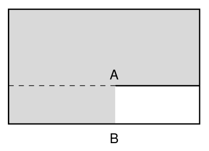
Figure 7: At low temperature the free energy for parallel plates (88) comes in part from an ideal gas filling the shaded region.

A nice way to interpret this result is to isolate the thermal Casimir energy associated with the gap. Proceeding as in section 3.1 we first subtract the free energy of a “big box” without any middle plate, given by

$$F_{\rm box}=-{\zeta(4)\over\pi^{2}}V_{\rm box}T^{4}+{\zeta(3)\over 8\pi}A_{\rm box}T^{3}-{\zeta(2)\over 16\pi}P_{\rm box}T^{2}$$ (89)

Next we subtract the thermal self-energy of the middle plate itself, as well as the thermal self-energy associated with the “$\dashv\,$” shaped junction on the right side of Fig. 7. These are give by

$$F_{\rm self}={\zeta(3)\over 4\pi}A_{\rm plate}T^{3}-{\zeta(2)\over 8\pi}L_{z}T^{2}$$ (90)

The bulk contribution to the free energy associated with the gap in the middle plate is then

$$F_{||,T}-F_{\rm box}-F_{\rm self} = {\zeta(4)\over\pi^{2}}\,V_{\rm ex}T^{4}-{\zeta(3)\over 8\pi}A_{\rm ex}T^{3}+{\zeta(2)\over 16\pi}P_{\rm ex}T^{2}$$

$$-{2\zeta(4)\over\pi^{3}}\,L_{z}b^{2}T^{4}\left(\log(2bT)+{\zeta^{\prime}(4)\over\zeta(4)}\right)+{{3\zeta(5)}\over{4\pi}}L_{z}b^{3}T^{5}+\cdots$$

Here $V_{\rm ex}$ is the excluded volume (the volume of the region between the two plates, shown in white in Fig. 7). Likewise $A_{\rm ex}=2A_{\rm plate}+bL_{z}$ is the excluded area (the surface area of the region in white, counting just the boundaries with solid lines), and $P_{\rm ex}=2L_{z}$ is the excluded perimeter. These geometrical terms have a simple interpretation, that at low temperatures thermal excitations cannot propagate in the region between the plates.

The leading diffractive contribution to the thermal free energy associated with the edge is

$$F^{\rm edge}_{||,T}=-{2\zeta(4)\over\pi^{3}}\,(bT)^{4}\left(\log(2bT)+{\zeta^{\prime}(4)\over\zeta(4)}\right){L_{z}\over{b^{2}}}$$ (92)

This contribution to the thermal free energy was studied by Gies and Weber in [8] using the world-line formalism. They observed that their numerical data was well fit, in the low temperature limit, by a power-law temperature dependence with a non-integer exponent $\sim T^{3.74}$. A numerical fit of our analytic result (92) in terms of a power-law dependence, for low temperatures, agrees well with the data in [8] and produces a similar exponent. However it is clear from our analysis that the non-integer power law found in [8] is actually due to a logarithmic temperature dependence of the form $T^{4}\log T$.

4 Conclusions

To summarize, we find that up to first order in diffractive effects, the thermal free energy at low temperature is

Perpendicular plates

$$F_{\perp,T}=-{\zeta(2)\over 8\pi}L_{z}T^{2}+{\zeta(3)\over 4\pi}L_{z}aT^{3}-{16\pi\zeta(3)\over 945}L_{z}a^{4}T^{6}+{\cal O}(T^{8})$$ (93)

This was given in (51).

Slit geometry

$$F_{\rm slit,T}={\zeta(3)\over 4\pi}L_{z}wT^{3}-{7\zeta(3)\over{90\pi}}L_{z}w^{2}T^{4}+{\cal O}(T^{6})$$ (94)

as given in (67).

Parallel plates
For parallel plates we find (3.3), which can be decomposed into an excluded volume contribution

$$F_{||,T}^{\rm ex}={\zeta(4)\over\pi^{2}}\,V_{\rm ex}T^{4}-{\zeta(3)\over 8\pi}A_{\rm ex}T^{3}+{\zeta(2)\over 16\pi}P_{\rm ex}T^{2}$$ (95)

and a diffractive edge contribution

$$F^{\rm edge}_{||,T}=-{2\zeta(4)\over\pi^{3}}\,(bT)^{4}\left(\log(2bT)+{\zeta^{\prime}(4)\over\zeta(4)}\right){L_{z}\over{b^{2}}}+{{3\zeta(5)}\over{4\pi}}L_{z}b^{3}T^{5}+\cdots$$ (96)

These results are consistent with the world-line numerical analysis in [7, 8] and they further capture subleading temperature dependence arising from diffractive effects. The result (96) provides an analytic understanding of the fractional power law observed in [8]. From a mathematical point of view we find it interesting that these non-trivial power laws are encoded in the non-local differential operators (9).

Our method is rather general and can be applied to many contexts in field theory where geometrical and thermal effects, and in particular the interplay between them, are important. For instance they could be used to study thermal corrections to the interaction between holes in a plate [10]. It is also straightforward to extend our results to higher dimensions. Another analytical approach to studying Casimir energies in geometries with edges and apertures is the multiple scattering method developed in [4]. It would be interesting to understand the relation between the expansion scheme developed here and the methods used in [4], as well as the convergence properties of these expansions at any temperature.

Acknowledgements

We are grateful to V.P. Nair for valuable discussions, and we thank Noah Graham, Robert Jaffe and Mohammad Maghrebi for hospitality and stimulating comments. This work was supported by U.S. National Science Foundation grants PHY-0855582 and PHY-0758008 and by PSC-CUNY grants.

Appendix A Ideal gas thermodynamics

The partition function for an ideal gas in a rectangular box of size $L_{x}\times b\times L_{z}$, with Dirichlet boundary conditions in the $L_{x}$ and $b$ directions and periodic boundary conditions around $L_{z}$ and $\beta$, is

$$-\log Z_{\rm 4d} = {1\over 2}{\rm Tr}\log\big{(}-\Box\big{)}$$ (97)

$$= {1\over 2}\sum\log\left[\left({{n\pi}\over L_{x}}\right)^{2}+\left({m\pi\over b}\right)^{2}+\left({2k\pi\over L_{z}}\right)^{2}+\left({2l\pi\over\beta}\right)^{2}\right]$$

where $n,m=1,2,\cdots$ and $k,l\in{\mathbb{Z}}$. As discussed in [3] appendix B, the renormalized partition function is, in the limit $L_{x},\,L_{z}\rightarrow\infty$,

$$-\log Z_{\rm 4d}=-{1\over 2}\int_{0}^{\infty}{ds\over s}\,\left({L_{x}\over\sqrt{4\pi s}}-{1\over 2}\right){L_{z}\over\sqrt{4\pi s}}\,\left[K_{P}(s,\beta)K_{D}(s,b)-{\beta\over\sqrt{4\pi s}}\left({b\over\sqrt{4\pi s}}-{1\over 2}\right)\right]$$ (98)

where the heat kernels associated with periodic (P) and Dirichlet (D) directions are

$$K_{P}(s,\beta) = {\beta\over\sqrt{4\pi s}}+{\beta\over\sqrt{\pi s}}\sum_{n=1}^{\infty}e^{-\beta^{2}n^{2}/4s}$$ (99)

$$K_{D}(s,b) = {b\over\sqrt{4\pi s}}-{1\over 2}+{b\over\sqrt{\pi s}}\sum_{n=1}^{\infty}e^{-b^{2}n^{2}/s}$$ (100)

The expansions (99), (100) are useful when $\beta$ or $b$ are large. For small $\beta$ or $b$ we use the Poisson-resummed forms

$$K_{P}(s,\beta) = 1+2\sum_{n=1}^{\infty}e^{-s4\pi^{2}n^{2}/\beta^{2}}$$ (101)

$$K_{D}(s,b) = \sum_{n=1}^{\infty}e^{-sn^{2}\pi^{2}/b^{2}}$$ (102)

To study the behavior at low temperature ($\beta\gg b$) we rewrite (98) as

$$-\log Z_{\rm 4d} = -{1\over 2}\int_{0}^{\infty}{ds\over s}\,\left({L_{x}\over\sqrt{4\pi s}}-{1\over 2}\right){L_{z}\over\sqrt{4\pi s}}\,\left[\left(K_{P}(s,\beta)-{\beta\over\sqrt{4\pi s}}\right)K_{D}(s,b)\right.$$ (103)

$$\hskip 85.35826pt+\left.{\beta\over\sqrt{4\pi s}}\left(K_{D}(s,b)-{b\over\sqrt{4\pi s}}+{1\over 2}\right)\right]$$

From (99), (102) the first line is exponentially suppressed at low temperatures, while the second line can be evaluated analytically. After integrating over $s$ we find

$$-\log Z_{\rm 4d} = -{\zeta(4)\beta L_{x}L_{z}\over 16\pi^{2}b^{3}}+{\zeta(3)\beta L_{z}\over 32\pi b^{2}}-{L_{x}L_{z}\over\sqrt{2\beta b^{3}}}\sum_{m,n=1}^{\infty}\left({m\over n}\right)^{3/2}K_{3/2}\left(mn\pi\beta/b\right)$$ (104)

$$+{L_{z}\over 2b}\sum_{m,n=1}^{\infty}{m\over n}K_{1}\left(mn\pi\beta/b\right)$$

The first two terms determine the Casimir energy at zero temperature associated with this geometry,

$$E^{\rm Casimir}_{T=0}=-{\zeta(4)L_{x}L_{z}\over 16\pi^{2}b^{3}}+{\zeta(3)L_{z}\over 32\pi b^{2}}$$ (105)

while the remaining terms give exponentially small thermal corrections.

To study the behavior at high temperatures ($\beta\ll b$) we rewrite (98) as

$$-\log Z_{\rm 4d} = -{1\over 2}\int_{0}^{\infty}{ds\over s}\,\left({L_{x}\over\sqrt{4\pi s}}-{1\over 2}\right){L_{z}\over\sqrt{4\pi s}}\,\left[K_{P}(s,\beta)\left(K_{D}(s,b)-{b\over\sqrt{4\pi s}}+{1\over 2}\right)\right.$$

$$\hskip 85.35826pt+\left.\left(K_{P}(s,\beta)-{\beta\over\sqrt{4\pi s}}\right)\left({b\over\sqrt{4\pi s}}-{1\over 2}\right)\right]$$ (106)

We use (101), (100) in the first line, while the second line can be evaluated analytically. Thus

$$-\log Z_{\rm 4d} = -{\zeta(4)\over\pi^{2}}VT^{3}+{\zeta(3)\over 8\pi}AT^{2}-{\zeta(2)\over 16\pi}PT-{\zeta(3)L_{x}L_{z}\over 16\pi b^{2}}+{\zeta(2)L_{z}\over 8\pi b}$$

$$-L_{x}L_{z}\sqrt{2\over b\beta^{3}}\sum_{m,n=1}^{\infty}\left({m\over n}\right)^{3/2}K_{3/2}\left(mn4\pi b/\beta\right)+{L_{z}\over\beta}\sum_{m,n=1}^{\infty}{m\over n}K_{1}\left(mn4\pi b/\beta\right)$$

Here $V=L_{x}bL_{z}$ is the volume of the box, $A=2(L_{x}+b)L_{z}$ is the surface area, and $P=4L_{z}$ is the “perimeter” (the length of the corners). The terms which are independent of $T$ come from $K_{P}(s,\beta)=1+\cdots$ in the first line; they give the Casimir energy associated with this geometry after dimensional reduction along the Euclidean time direction. The volume term in (A) gives the usual extensive free energy of an ideal gas; note that only Dirichlet boundaries count towards the surface area.

One can perform a similar analysis in 2+1 dimensions. For a gas in a box of size $b\times L_{z}$, with Dirichlet boundary conditions in $b$ and periodic boundary conditions around $L_{z}$ and $\beta$, the starting point is, for $L_{z}\rightarrow\infty$,

$$-\log Z_{\rm 3d}=-{1\over 2}\int_{0}^{\infty}{ds\over s}\,{L_{z}\over\sqrt{4\pi s}}\,\left[K_{P}(s,\beta)K_{D}(s,b)-{\beta\over\sqrt{4\pi s}}\left({b\over\sqrt{4\pi s}}-{1\over 2}\right)\right]$$ (108)

Proceeding as before, at low temperatures we have

$$-\log Z_{\rm 3d}=-{\zeta(3)\beta L_{z}\over 16\pi b^{2}}-{L_{z}\over b}\sum_{m,n=1}^{\infty}{m\over n}K_{1}(mn\pi\beta/b)$$ (109)

The first term gives the Casimir energy at zero temperature in 2+1 dimensions, while the remaining terms are exponentially small thermal corrections. At high temperatures the steps leading to (A) give

$$-\log Z_{\rm 3d}=-{\zeta(3)bL_{z}\over 2\pi\beta^{2}}+{\pi L_{z}\over 12\beta}-{\pi L_{z}\over 24b}-{2L_{z}\over\beta}\sum_{m,n=1}^{\infty}{m\over n}K_{1}(mn4\pi b/\beta)$$ (110)

Appendix B Direct free energy for parallel plates

In this appendix we compute the second piece of the direct free energy for parallel plates (72). The 2d partition function is

$$-\log Z_{\rm 2d}^{(2)} = -{1\over 2}\sum_{n=1}^{\infty}\log\left(1-e^{-2b\sqrt{(n\pi/a)^{2}+\mu^{2}}}\right)$$

$$= -{a\over 2\pi}\int_{0}^{\infty}dk\,\log\left(1-e^{-2b\sqrt{k^{2}+\mu^{2}}}\right)+{1\over 4}\log\left(1-e^{-2b\mu}\right)+{\cal O}(1/a)$$

where we used the Euler-Maclaurin summation formula to obtain the behavior for large $a$. Letting $x=b\sqrt{k^{2}+\mu^{2}}$ and integrating by parts this is

$${a\over\pi b}\int_{\mu b}^{\infty}dx\,\sqrt{x^{2}-\mu^{2}b^{2}}\,\left(e^{2x}-1\right)^{-1}+{1\over 4}\log\left(1-e^{-2b\mu}\right)+{\cal O}(1/a)$$ (111)

The non-analytic behavior of the integral as $\mu b\rightarrow 0$ can be obtained by the method explained below (43). Keeping only terms which are non-analytic as functions of $\mu^{2}$, we find that

$$-\log Z_{\rm 2d}^{(2)}={1\over 4}\log\mu b-{1\over 4}\mu(a+b)-{1\over 4\pi}ab\mu^{2}\log\mu b+{\cal O}\big{(}(\mu b)^{4}\big{)}$$ (112)

Substituting this in (31), the four dimensional free energy is

$$F_{\rm 4d}^{(2)} = {L_{z}\over\pi}\sum_{l=1}^{\infty}\int_{0}^{\infty}\mu d\mu\,J_{0}(\beta\mu l)\left({1\over 4}\log\mu b-{1\over 4}\mu(a+b)-{1\over 4\pi}ab\mu^{2}\log\mu b\right)$$ (113)

$$= -{\zeta(2)\over 4\pi}\,L_{z}T^{2}+{\zeta(3)\over 4\pi}L_{z}(a+b)T^{3}-{\zeta(4)\over\pi^{2}}L_{z}abT^{4}$$

Another approach to evaluating (72) is to begin from the partition function for a Bose gas in a box of size $a\times L_{z}\times 2b$, with Dirichlet boundary conditions in $a$ and periodic boundary conditions around $L_{z}$ and $2b$. With $a,L_{z}\rightarrow\infty$ this is

$$-\log Z_{\rm Bose}=-{1\over 2}\int_{0}^{\infty}{ds\over s}\,\left({a\over\sqrt{4\pi s}}-{1\over 2}\right){L_{z}\over\sqrt{4\pi s}}\,\left[K_{P}(s,\beta)K_{P}(s,2b)-{\beta\over\sqrt{4\pi s}}{2b\over\sqrt{4\pi s}}\right]$$ (114)

This partition function is manifestly symmetric under exchange $\beta\leftrightarrow 2b$. Evaluating it at large $\beta$ as in appendix A, we find

$$-\log Z_{\rm Bose} = -{\zeta(4)aL_{z}\beta\over 8\pi^{2}b^{3}}+{\zeta(3)L_{z}\beta\over 16\pi b^{2}}-{\zeta(3)aL_{z}\over 2\pi\beta^{2}}+{\zeta(2)L_{z}\over 2\pi\beta}$$

$$+(\hbox{\rm exponentially small thermal corrections})$$

while evaluating it at small $\beta$ gives

$$-\log Z_{\rm Bose} = -{2\zeta(4)aL_{z}b\over\pi^{2}\beta^{3}}+{\zeta(3)L_{z}b\over 2\pi\beta^{2}}-{\zeta(3)aL_{z}\over 8\pi b^{2}}+{\zeta(2)L_{z}\over 4\pi b}$$

$$+(\hbox{\rm exponentially small finite size corrections})$$

Regarding $2b$ as the Euclidean time direction and working in a Hamiltonian picture we have

$$-\log Z_{\rm Bose}={\rm Tr}\log\left[2\sinh\big{(}b\sqrt{(n\pi/a)^{2}+(2k\pi/L_{z})^{2}+(2l\pi/\beta)^{2}}\big{)}\right]$$ (117)

After multiplying by an overall factor of $-1/2$, this can be identified with the contribution (72) to the direct free energy for parallel plates, except that in (72) the zero point energy has been suppressed. That is, we can identify

$$\beta F^{(2)}_{\rm 4d}=-{1\over 2}\left(-\log Z_{\rm Bose}-2bE_{\rm Casimir}\right)$$ (118)

where the Casimir energy at zero “temperature” (meaning $2b\rightarrow\infty$) for this geometry is, from (B),

$$E_{\rm Casimir}=-{\zeta(4)aL_{z}\over\pi^{2}\beta^{3}}+{\zeta(3)L_{z}\over 4\pi\beta^{2}}$$ (119)

Using (B), we find that (118) reproduces the temperature dependence seen in (113), and in fact shows that corrections to (113) are exponentially small.

References

• [1] H.B.G. Casimir, “On the attraction between two perfectly conducting plates”, Proc. K. Ned. Akad. Wet 51, 793 (1948); H.B.G. Casimir and D. Polder, “The influence of retardation on the London-van der Waals forces”, Phys. Rev. 73, 360 (1948).
• [2] K.A. Milton, Recent developments in Casimir effect, J. Phys. Conf. Ser. 161, 012001 (2009); K. A. Milton, The Casimir Effect: Physical Manifestations of Zero-Point Energy (World Scientific, 2001); M. Bordag, U. Mohideen and V.M. Mostepanenko, Phys. Rept. 353, 1 (2001); M. Bordag, G.L. Klimchitskaya, U. Mohideen and V.M. Mostepanenko, Advances in the Casimir Effect (International Series of Monographs on Physics, 2009).
• [3] D. Kabat, D. Karabali, and V. P. Nair, “Edges and diffractive effects in Casimir energies”, Phys. Rev. D81, 125013 (2010).
• [4] N. Graham, A. Shpunt, T. Emig, S. J. Rahi, R. L. Jaffe and M. Kardar, “Casimir force at a knife’s edge”, Phys. Rev. D81, 061701 (2010); M. F. Maghrebi, S. J. Rahi, T. Emig, N. Graham, R. L. Jaffe, M. Kardar, “Casimir force between sharp-shaped conductors”, Proc.Nat.Acad.Sci. 108, 6867 (2011); M. F. Maghrebi, N. Graham, “Electromagnetic Casimir energies of semi-infinite planes”, Europhys.Lett. 95, 14001 (2011); N. Graham, A. Shpunt, T. Emig, S. J. Rahi, R. L. Jaffe, M. Kardar, “Electromagnetic forces of parabolic cylinder and knife-edge geometries”, Phys.Rev. D83, 125007 (2011).
• [5] K. A. Milton, E. K. Abalo, P. Parashar, N. Pourtolami, I. Brevik, S. A. Ellingsen, “Casimir-Polder repulsion near edges: wedge apex and a screen with an aperture”, Phys. Rev. A 83, 062507 (2011).
• [6] H. Gies and K. Klingmüller, “Casimir edge effects”, Phys. Rev. Lett. 96, 220401 (2006).
• [7] K. Klingmüller and H. Gies, “Geothermal Casimir phenomena”, J. Phys. A 41, 164042 (2008).
• [8] A. Weber and H. Gies, “Interplay between geometry and temperature for inclined Casimir plates”, Phys.Rev. D80, 065033 (2009); H. Gies and A. Weber, “Geometry-temperature interplay in the Casimir effect”, Int.J.Mod.Phys. A25, 2279 (2010).
• [9] R. L. Frank and L. Geisinger, “Refined semiclassical asymptotics for fractional powers of the Laplace operator”, arXiv:1105.5181 [math.SP].
• [10] D. Kabat, D. Karabali, V. P. Nair, “On the Casimir interaction between holes”, Phys. Rev.  D82, 025014 (2010).