Generalized Maneuvers in Route Planning

Abstract

We study an important practical aspect of the route planning problem in real-world road networks – maneuvers. Informally, maneuvers represent various irregularities of the road network graph such as turn-prohibitions, traffic light delays, round-abouts, forbidden passages and so on. We propose a generalized model which can handle arbitrarily complex (and even negative) maneuvers, and outline how to enhance Dijkstra’s algorithm in order to solve route planning queries in this model without prior adjustments of the underlying road network graph.

1 Introduction

Since mass introduction of GPS navigation devices, the route planning problem, has received considerable attention. This problem is in fact an instance of the well-known single pair shortest path (SPSP) problem in graphs representing real-world road networks. However, it involves many challenging difficulties compared to ordinary SPSP. Firstly, classical algorithms such as Dijkstra’s [4], A* [6] or their bidirectional variants [11] are not well suited for the route planning despite their optimality in wide theoretical sense. It is mainly because graphs representing real-world road networks are so huge that even an algorithm with linear time and space complexity cannot be feasibly run on typical mobile devices.

Secondly, these classical approaches disregard certain important aspects of real-world road networks, namely route restrictions, traffic regulations, or actual traffic info. Hence a route found by such algorithms might not be optimal or not even feasible. Additional attributes are needed in this regard.

The first difficulty has been intensively studied in the past decade, and complexity overheads of classical algorithms have been largely improved by using various preprocessing approaches. For a brief overview, we refer the readers to [2, 3, 12] or our [7]. In this paper we focus on the second mentioned difficulty as it is still receiving significantly less attention.

1.0.1 Related Work.

The common way to model required additional attributes of road networks is with so called maneuvers; Definition 1. Maneuvers do not seem to be in the center of interest of route-planning research papers: They are either assumed to be encoded into the underlying graph of a road network, or they are addressed only partially with rather simple types of restriction attributes such as turn-penalties and path prohibitions.

Basically, the research directions are represented either by modifications of the underlying graph during preprocessing [8, 10, 15], or by adjusting a query algorithm [9, 13] in order to resolve simple types of restrictions during queries.

The first, and seemingly the simplest, solution is commonly used as it makes a road network graph maneuver-free and so there is no need to adjust the queries in any way. Unfortunately, it can significantly increase the size of the graph [14]; for instance, replacing a single turn-prohibition can add up to eight new vertices in place of one original [5]. A solution like this one thus conflicts with the aforementioned (graph-size) objectives. Another approach [1] uses so-called dual graph representation instead of the original one, where allowed turns are modeled by dual edges.

To summarize, a sufficiently general approach for arbitrarily complex maneuvers seems to be missing in the literature despite the fact that such a solution could be really important. We would like to emphasize that all the cited works suffer from the fact that they consider only “simple” types of maneuvers.

1.0.2 Our Contribution.

Firstly, we introduce a formal model of a generic maneuver – from a single vertex to a long self-intersecting walk – with either positive or negative effects (penalties); being enforced, recommended, not recommended or even prohibited. Our model can capture virtually any route restriction, most traffic regulations and even some dynamic properties of real-world road networks.

Secondly, we integrate this model into Dijkstra’s algorithm, rising its worst-case time complexity only slightly (depending on a structure of maneuvers). The underlying graph is not modified at all and no preprocessing is needed. Even though our idea is fairly simple and relative easy to understand, it is novel in the respect that no comparable solution has been published to date. Furthermore, some important added benefits of our algorithm are as follows:

• It can be directly used bidirectionally with any alternation strategy using an appropriate termination condition; it can be extended also to the A* algorithm by applying a “potential function to maneuver effects”.

• Many route planning approaches use Dijkstra or A* in the core of their query algorithms, and hence our solution can be incorporated into many of them (for example, those based on a reach, landmarks or various types of separators) quite naturally under additional assumptions.

• Our algorithm tackles maneuvers “on-line” – that is no maneuver is processed before it is reached. And since the underlying graph of a road network is not changed (no vertices or edges are removed or added), it is possible to add or remove maneuvers dynamically even during queries to some extent.

2 Maneuvers: Basic Terms

A (directed) graph $G=(V,E)$ is a pair of a finite set $V$ of vertices and a finite multiset $E\subseteq V\times V$ of edges (self-loops and parallel edges are allowed). The vertex set of $G$ is referred to as $V(G)$, its edge multiset as $E(G)$. A subgraph $H$ of a graph $G$ is denoted by $H\subseteq G$.

A walk $P\in G$ is an alternating sequence of vertices and edges $(u_{0},e_{1},u_{1},\ldots,$ $e_{k},u_{k})\subseteq G$ such that $e_{i}=(u_{i-1},u_{i})$ for $i=1,\ldots,k$, the multiset of all edges of a walk $P$ is denoted by $E(P)$. A concatenation $P_{1}.\,P_{2}$ of walks $P_{1}=(u_{0},e_{1},u_{1},\ldots,e_{k},u_{k})$ and $P_{2}=(u_{k},e_{k+1},u_{k+1},\ldots,e_{l},u_{l})$ is the walk $(u_{0},e_{1},u_{1},$ $\ldots,e_{k},u_{k},e_{k+1},\ldots,e_{l},u_{l})$. If $P_{2}=(u,f,v)$ represents a single edge, we write $P_{1}.\,f$. If edges are clear from the graph, then we write a walk simply as $(u_{0},u_{1},\dots,u_{k})$.

A walk $Q$ is a prefix of another walk $P$ if $Q$ is a subwalk of $P$ starting with the same index, and analogically with suffix. The prefix set of a walk $P=(u_{0},e_{1},\ldots,e_{k},u_{k})$ is $\mathit{Prefix}(P)=\{(u_{0},e_{1},\ldots,e_{i},u_{i})|\>0\leq i\leq k\},$ and analogically $\mathit{Suf\!fix}(P)=\{(u_{i},e_{i+1},\ldots,e_{k},u_{k})|\>0\leq i\leq k\}$. A prefix (suffix) of a walk $P$ thus is a member of $\mathit{Prefix}(P)$ ($\mathit{Suf\!fix}(P)$), and it is nontrivial if $i\geq 1$.

The weight of a walk $P\subseteq G$ with respect to a weighting $w:E(G)\mapsto\mathbb{R}$ of $G$ is defined as $\sum_{e\in E(P)}w(e)$ and denoted by $|P|_{w}$. A distance from $u$ to $v$ in $G$, $\delta_{w}(u,v)$, is the minimum weight of a walk $P=(u,\ldots,v)\subseteq G$ over all such walks and $P$ is then called optimal (with respect to weighting $w$). If there no such walk then $\delta_{w}(u,v)=\infty$. A path is a walk without repeating vertices and edges.

Virtually any route restriction or traffic regulation in a road network, such as turn-prohibitions, traffic lights delays, forbidden passages, turn-out lanes, suggested directions or car accidents by contrast, can be modeled by maneuvers – walks having extra (either positive or negative) “cost effects”. Formally:

Definition 1 (Maneuver)

A maneuver $M$ of $G$ is a walk in $G$ that is assigned a penalty $\Delta(M)\!\in\!\mathbb{R}\!\cup\!\infty$. A set of all maneuvers of $G$ is denoted by ${\cal{M}}$.

Remark 1

A maneuver with a negative or positive penalty is called negative or positive, respectively. Furthermore, there are two special kinds of maneuvers the restricted ones of penalty 0 and the prohibited ones of penalty $\infty$.

The cost effect of a maneuver is formalized next:

Definition 2 (Penalized Weight)

Let $G$ be a graph with a weighting $w$ and a set of maneuvers $\cal{M}$. The penalized weight of a walk $P\subseteq G$ containing the maneuvers $M_{1},\ldots,M_{r}\in{\cal{M}}$ as subwalks is defined as $|P|_{w}^{\cal{M}}=|P|_{w}+\sum_{i=1}^{r}\Delta(M_{i})$.

Then, the intended meaning of maneuvers in route planning is as follows.

• If a driver enters a restricted maneuver, she must pass it completely (cf. Definition 3); she must obey the given direction(s) regardless of the cost effect. Examples are headings to be followed or specific round-abouts.

• By contrast, if a driver enters a prohibited maneuver, she must not pass it completely. She must get off it before reaching its end, otherwise it makes her route infinitely bad. Examples are forbidden passages or temporal closures.

• Finally, if a driver enters a positive or negative maneuver, she is not required to pass it completely; but if she does, then this will increase or decrease the cost of her route accordingly. Negative maneuvers make her route better (more desirable) and positive ones make it worse. Examples of positive maneuvers are, for instance, traffic lights delays, lane changes, or left-turns. Examples of negative ones are turn-out lanes, shortcuts, or implicit routes.

Definition 3 (Valid Walk)

Let $G,w,\cal{M}$ be as in Definition 2. A walk $P$ in $G$ is valid if and only if $|P|_{w}^{\cal{M}}<\infty$ and, for any restricted maneuver $M\in\cal{M}$, it holds that if a nontrivial prefix of $M$ is a subwalk of $P$, then whole $M$ is a subwalk of $P$ or a suffix of $P$ is contained in $M$ (that is $P$ ends there).

We finally get to the summarizing definition. A structure of a road network is naturally represented by a graph $G$ such that the junctions are represented by $V(G)$ and the roads by $E(G)$. The chosen cost function (for example travel time, distance, expenses) is represented by a non-negative weighting $w:E(G)\mapsto\mathbb{R}^{+}_{0}$ assigned to $G$, and the additional attributes such as traffic regulations are represented by maneuvers as above. We say that two walks $Q_{1},Q_{2}$ are divergent if, up to symmetry between $Q_{1},Q_{2}$, a nontrivial prefix of $Q_{1}$ is contained in $Q_{2}$ but the whole $Q_{1}$ is not a subwalk of $Q_{2}$. Moreover, we say that $Q_{2}$ overhangs $Q_{1}$ if a nontrivial prefix of $Q_{2}$ is a suffix of $Q_{1}$ (particularly, $E(Q_{1})\cap E(Q_{2})\neq\emptyset$).

Definition 4 (Road Network)

Let $G$ be a graph with a non-negative weighting $w$ and a set of maneuvers $\cal M$. A road network is the triple $(G,w,{\cal M})$. Furthermore, it is called proper if:

• no two restricted maneuvers in $\cal M$ are divergent,

• no two negative maneuvers in $\cal M$ overhang one another, and

• for all $N\in{\cal{M}}$, $\Delta(N)\geq-|N|_{w}^{{\cal{M}}\setminus\{N\}}$ (that is, the penalized weight of every walk in $G$ is non-negative).

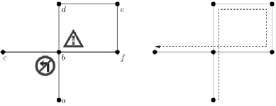
Figure 1: A road network containing maneuvers $M_{1}=(a,ab,b,bc,c)$ with $\Delta(M_{1})=\infty$ (prohibited left turn) and $M_{2}=(a,ab,b,bf,f)$ with $\Delta(M_{2})=1$ (right turn traffic lights delay). All edges have weight 1. The penalized weight of the walk $(a,ab,b,bc,c)$ is $2+\infty$, the penalized weight of the walk $(a,ab,b,bf,f,fe,e,ed,d,db,b,bd,c)$ is $6+1$. Therefore the optimal walk (with respect to the penalized weight) from $a$ to $c$ is $(a,ab,b,bd,d,de,e,ef,f,fb,b,bc,c)$ with the penalized weight $6+0$.

Within a road network, only valid walks (Definition 3) are allowed further, and the distance from $u$ to $v$, $\delta_{w}^{\cal{M}}(u,v)$, is the minimum penalized weight (Definition 2) of a valid walk $P=(u,\ldots,v)\subseteq G$; such a walk $P$ is then called optimal with respect to the penalized weight. If there is no such walk, then $\delta_{w}^{\cal{M}}(u,v)=\infty$. See Fig. 1.

Motivation for the required properties i.–iii. in Definition 4 is of both natural and practical character: As for i., it simply says that no two restricted maneuvers are in a conflict (that is no route planning deadlocks). Point ii. concerning only negative maneuvers is needed for a fast query algorithm, and it is indeed a natural requirement (to certain extent, overhanging maneuvers can be modeled without overhangs). We remark that other studies usually allow no negative maneuvers at all. Finally, iii. states that no negative maneuvers can result in a negative overall cost of any walk – another very natural property. In informal words, a negative penalty of a maneuver somehow “cannot influence” suitability of a route before entering and after exiting the maneuver.

2.1 Strongly Connected Road Network

The traditional graph theoretical notion of strong connectivity also needs to be refined, it must suit our road networks to dismiss possible route planning traps now imposed by maneuvers.

First, we need to define a notion of a “context” of a vertex $v$ in $G$ – a maximal walk in $G$ ending at $v$ such that it is a proper prefix of a maneuver in $\cal M$, or $\emptyset$ otherwise. A set of all such walks for $v$ is denoted by ${\cal{X}}_{\cal{M}}$. For example, on the road network depicted on Fig. 1, ${\cal{X}}_{\cal M}(b)=\{(a,b),\emptyset\}$. More formally:

Definition 5

Let $\cal M$ be a set of maneuvers. We define

$${\cal{X}}_{{\cal{M}}}(v)\stackrel{{\scriptstyle\textrm{\tiny{def}}}}{{=}}\big{\{}X\in\mathit{Prefix}^{<}({\cal M})\,|(v)\in\mathit{Suf\!fix}(X)\big{\}}\cup\{\emptyset\}$$

$$\mathit{Prefix}^{<}(M)\stackrel{{\scriptstyle\textrm{\tiny{def}}}}{{=}}\mathit{Prefix}(M)\setminus\{M\},\quad\mathit{Prefix}^{<}({\cal M})\stackrel{{\scriptstyle\textrm{\tiny{def}}}}{{=}}\bigcup\nolimits_{M\in\cal M}\mathit{Prefix}^{<}(M).$$

This ${\cal{X}}_{{\cal{M}}}(v)$ is the maneuver-prefix set at $v$, that is the set of all proper prefixes of walks from $\cal M$ that end right at $v$, including the mandatory empty walk. An element of ${\cal{X}}_{{\cal{M}}}(v)$ is called a context of the position $v$ within the road network.

The reverse graph $G^{R}$ of $G$ is a graph on the same set of vertices with all of the edges reversed. Let $(G,w,{\cal{M}})$ be a road network, a reverse road network is defined as $(G^{R},w^{R},{\cal{M}}^{R})$, where $w^{R}:E(G^{R})\mapsto\mathbb{R}_{0}^{+}$, $\forall(u,v)\in E(G^{R}):\,w^{R}(u,v)=w(v,u)$ and ${\cal{M}}^{R}=\{M^{R}|M\in{\cal{M}}\}$, $\forall M^{R}\in{\cal{M}}^{R}:\,\Delta(M^{R})=\Delta(M)$.

Definition 6

A road network $(G,w,{\cal M})$ is strongly connected if, for every pair of edges $e=(u^{\prime},u),\>f=(v,v^{\prime})\in E(G)$ and for each possible context $X=X_{1}\cdot\,e\in{\cal X}_{\cal M}(u)$ of $u$ in $G$ and each one of $v$ in $G^{R}$, that is  $Y^{R}=Y_{1}^{R}.\,f^{R}\in{\cal X}_{{\cal M}^{R}}(v)$, there exists a valid walk starting with $X$ and ending with $Y$.

We remark that Definition 6 naturally corresponds to strong connectivity in an amplified road network modeling the maneuvers within underlying graph.

3 Route Planning Queries

At first, let us recall classical Dijkstra’s algorithm [4]. It solves SPSP problem a graph $G$ with a non-negative weighting $w$ for a pair $s,t\in V(G)$ of vertices.

• The algorithm maintains, for all $v\in V(G)$, a (temporary) distance estimate of the shortest path from $s$ to $v$ found so far in $d[v]$, and a predecessor of $v$ on that path in $\pi[v]$.

• The scanned vertices, that is those with $d[v]=\delta_{w}(s,v)$, are stored in the set $T$; and the reached but not yet scanned vertices, that is those with $\infty>d[v]\geq\delta_{w}(s,v)$, are stored in the set $Q$.

• The algorithm work as follows: it iteratively picks a vertex $u\in Q$ with minimum value $d[u]$ and relaxes all the edges $(u,v)$ leaving $u$. Then $u$ is removed from $Q$ and added to $T$. Relaxing an edge $(u,v)$ means to check if a shortest path estimate from $s$ to $v$ may be improved via $u$; if so, then $d[v]$ and $\pi[v]$ are updated. Finally, $v$ is added into $Q$ if is not there already.

• The algorithm terminates when $t$ is scanned or when $Q$ is empty.

Time complexity depends on the implementation of $Q$; such as it is ${\cal{O}}(|E(G)|+|V(G)|\log|V(G)|)$ with the Fibonacci heap.

3.1 $\cal{M}$-Dijkstra’s Algorithm

In this section we will briefly sketch the core ideas of our natural extension of Dijkstra’s algorithm. We refer a reader to Algorithm 1 for a full-scale pseudocode of this $\cal{M}$-Dijkstra’s algorithm.

1. Every vertex $v\in V(G)$ scanned during the algorithm is considered together with its context $X\in{\cal X}_{\cal M}(v)$ (Definition 5); that is as a pair $(v,X)$. The intention is for $X$ to record how $v$ has been reached in the algorithm, and same $v$ can obviously be reached and scanned more than once, with different contexts. For instance, $b$ can be reached with the empty or $(a,b)$ contexts on the road network depicted on Fig. 1.

2. Temporary distance estimates are stored in the algorithm as $d[v,X]$ for such vertex-context pairs $(v,X)$. At each step the algorithm selects a next pair $(u,Y)$ such that it is minimal with respect to the following partial order $\leq_{\cal M}$.

   Remark 2

   Partial order $\leq_{\cal M}$:

   $$(v_{1},X_{1})\leq_{\cal M}(v_{2},X_{2})\stackrel{{\scriptstyle\textrm{\tiny{def}}}}{{\Longleftrightarrow}}\left.\begin{array}[]{ll}\big{(}d[v_{1},X_{1}]<d[v_{2},X_{2}]&\lor\\[2.0pt] (d[v_{1},X_{1}]=d[v_{2},X_{2}]&\land\>X_{1}\in\mathit{Suf\!fix}(X_{2})\,)\big{)}.\end{array}\right.$$

3. Edge relaxation from a selected vertex-context pair $(u,Y)$ respects all maneuvers related to the context $Y$ (there can be more such maneuvers). If one of them is restricted, then only its unique (cf. Definition 4, i.) subsequent edge is taken, cf. Algorithm 1, RestrictedDirection.

   Otherwise, every edge $f=(u,v)$ is relaxed such that the distance estimate at $v$ – together with its context as derived from the concatenation $(Y.\,f)$ – is (possibly) updated with the weight $w(f)$ plus the sum of penalties of all the maneuvers in $(Y.\,f)$ ending at $v$, cf. Algorithm 1, Relax.

4. If an edge relaxed is the first one of a negative maneuver, a specific process is executed before scanning the next vertex-context pair. See below.

3.2 Processing Negative Maneuvers

Note that the presence of a maneuver of negative penalty may violate the basic assumption of ordinary Dijkstra’s algorithm; that relaxing an edge never decreases the nearest temporary distance estimate in the graph. An example of such a violation can be seen in Fig. 2, for instance, at vertex $v_{5}$ which would not be processed in its correct place by ordinary Dijkstra’s algorithm. That is why a negative maneuver $M$ must be processed by $\cal{M}$-Dijkstra’s algorithm at once – whenever its starting edge is relaxed, cf. Algorithm 1, ProcessNegative.

Suppose that an edge $f=(u,v)$ is relaxed from a selected vertex-context pair $(u,X)$ and there is a negative maneuver $M=(v_{0},f_{1},v_{1},\ldots,v_{n-1},f_{n},v_{n})$, $u=v_{0}$, $v=v_{1}$ starting with $f$ (that is $f=f_{1}$), processing negative maneuver $M$ works as follow:

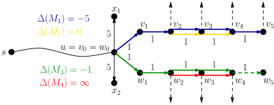
Figure 2: A road network containing two negative maneuvers, $M_{1}=(v_{0},\ldots,v_{5})$ and $M_{3}=(w_{0},\ldots,,w_{5})$, a restricted maneuver $M_{2}=(v_{2},v_{3},v_{4})$, and a prohibited maneuver $M_{4}=(w_{2},w_{3},w_{4})$. When $u$ is being processed (with its implicit context), $x_{1},x_{2}$ and $v_{1},w_{1}$ are relaxed normally. Furthermore, negative maneuver processing is executed for both $M_{1}$ and $M_{3}$. As a result, $v_{5}$ will be immediately reached and inserted to $Q$ with distance estimate equal to that of $u$ which is less than those of $x_{1},x_{2}$ (5 from $u$) and of $v_{1},w_{1}$ (1 from $u$). On the other hand, $w_{5}$ will not be reached in the process because the distance estimate of $w_{4}$ bounces to $\infty$ while handling $M_{4}$.

1. Vertex-context pairs $(v_{i},X_{i}),0\leq i\leq n$ along $M$ are scanned one by one towards the end of $M$. The other vertices leaving these $v_{i}$ are ignored.

2. Scanned vertex-context pairs are added to $Q$ and their distance estimates are updated, but none of them is added into $T$. They must be properly scanned during the main loop of the algorithm.

3. This process terminates when the end $(v_{n},X_{n})$ is reached or the distance estimate of some $(v_{i},X_{i})$ bounces to $\infty$ (that is there is a prohibited maneuver ending at $v_{i}$) or when some restricted maneuver forces us to get off $M$ (and thus $M$ cannot be completed).

Algorithm 1  $\cal{M}$-Dijkstra’s Algorithm

0:  A proper road network $(G,w,{\cal M})$ and vertices $s,t\in V(G)$.

0:  A valid walk from $s$ to $t$ in $G$ optimal with respect to the penalized weight.

${\cal{M}}$-Dijkstra$(G,w,{\cal{M}},s,t)$

1:  for all $v\in V(G)$, $X\in{\cal X}_{\cal M}(v)$ do /* Initialization. */

2:        $d[v,X]\leftarrow\infty;~{}\pi[v,X]\leftarrow\bot$

3:  done

4:  $d[s,\emptyset]\leftarrow 0$;  $Q\leftarrow\{(s,\emptyset)\}$;  $T\leftarrow\emptyset$

5:  if $(s)\in{\cal{M}}$ then $d[s,\emptyset]\leftarrow d[s,\emptyset]+\Delta(s)$ fi /* The main loop starts at $(s,\emptyset)$ and terminates when either all reachable vertex-context pairs have been scanned or when $t$ is reached with some of its contexts. */

6:  while $Q\neq\emptyset\land[\not\exists\,X\in{\cal{X}}_{\cal{M}}(t)$ s.t. $(t,X)\in T]$ do

7:        $(u,X)\leftarrow\min_{\leq_{\cal M}}(Q)$; $Q\leftarrow Q\setminus\{(u,X)\}$ /* Recall $\leq_{\cal{M}}$ (Remark 2) */

8:        $F\leftarrow\textsc{RestrictedDirection}(u,X)$ /* Possible restricted dir. from $u$. */

9:        if $F=\emptyset$ then $F\leftarrow\{(u,v)\in E(G)\,|\,v\in V(G)\}$ fi

10:        for all $f=(u,v)\in F$ do

11:              Relax$(u,X,f,v)$

12:              for all $M=(u,f,v,\ldots)\in{\cal{M}}$ s.t. $\Delta(M)<0\,\wedge\,|E(M)|>1$ do

13:                    ProcessNegative$\,(X,M)$

14:              done/* Negative man. starting with $f$ are processed separately. */

15:        done

16:        $T\leftarrow T\cup\{(u,X)\}$

17:  done

18:  ConstructWalk$\,(G,d,\pi)$ /* Use “access” information stored in $\pi[v,X]$. */

LongestPrefix$\,(P):\>\textrm{a walk }P^{\prime}\subseteq G$

0:   /* The longest (proper) prefix of some maneuver contained as a suffix of $P$ */

1:  $\begin{array}[]{l}P^{\prime}\leftarrow\max_{\subseteq}\big{[}\,(\mathit{Suf\!fix}(P)\cap\mathit{Prefix}^{<}({\cal{M}}))\cup\{\emptyset\}\big{]}\\ ~{}~{}~{}~{}~{}~{}~{}~{}~{}~{}~{}~{}~{}~{}~{}~{}~{}~{}~{}\mbox{where }\mathit{Prefix}^{<}({\cal M})\stackrel{{\scriptstyle\textrm{\tiny{def}}}}{{=}}\bigcup\nolimits_{M\in\cal M}\mathit{Prefix}(M)\setminus\{M\}\end{array}$

2:  return  $P^{\prime}$

RestrictedDirection$(u,X):\>F\subseteq E(G)$

0:   /* Looking for edge $f$ leaving $u$ that follows in a restricted man. in context $X$.*/

1:  $\begin{array}[]{l}F\leftarrow\{f=(u,v)\in E(G)\,|\,~{}\exists\textrm{ restricted }R\in{\cal{M}}:\\ ~{}~{}~{}~{}~{}~{}~{}~{}~{}~{}~{}~{}~{}~{}~{}~{}~{}~{}~{}E(X)\cap E(R)\neq\emptyset\,\land\mathit{Suf\!fix}(X.\,f)\cap\mathit{Prefix}(R)\neq\emptyset\}\end{array}$

2:  return  $F$

Relax$\,(u,X,f,v)$

0:   /* Relaxing an edge $f$ from vertex $u$ with context $X$. */

1:  $\delta\leftarrow w(f)+\sum_{N\in{\cal{N}}}\Delta(N)$  where ${\cal{N}}={\cal{M}}\cap\mathit{Suf\!fix}(X.\,f)$

2:  $X^{\prime}\leftarrow\textsc{LongestPrefix}(X.f)$

3:  if $d[u,X]+\delta<d[v,X^{\prime}]$ then

4:        $Q\leftarrow Q\cup\{(v,X^{\prime})\}$;  $d[v,X^{\prime}]\leftarrow d[u,X]+\delta$;  $\pi[v,X^{\prime}]\leftarrow(u,X)$

5:  fi

ProcessNegative$(X,\,M=(v_{0},e_{1},\ldots,e_{n},v_{n})\,)$

1:  $i\leftarrow 1;\,X_{0}\leftarrow X;\,F\leftarrow\emptyset$ /* Relaxing sequentially all the edges of $M$. */

2:  while $i\leq n\land d[v_{i-1},X_{i}]<\infty\land F=\emptyset$ do

3:        Relax$(v_{i-1},X_{i-1},e_{i},v_{i})$

4:        $X_{i}\leftarrow\textsc{LongestPrefix}(X_{i-1}.e_{i})$; $F\leftarrow\textsc{RestrictedDirection}(v_{i},X_{i})\setminus\{e_{i+1}\}$

5:        $i\leftarrow i+1$

6:  done

3.3 Correctness and Complexity Analysis

Assuming validity of Definition 4  ii. in a proper road network, correctness of above $\cal{M}$-Dijkstra’s algorithm can be argued analogously to a traditional proof of Dijkstra’s algorithm. Hereafter, the time complexity growth of the algorithm depends solely on the number of vertex-context pairs.

Theorem 3.1

Let a proper road network $(G,w,\cal{M})$ and vertices $s,t\in V(G)$ be given. ${\cal{M}}$-Dijkstra’s algorithm (Algorithm 1) computes a valid walk from $s$ to $t$ in $G$ optimal with respect to the penalized weight, in time ${\cal O}\big{(}c^{2}_{\cal M}|E(G)|+c_{\cal M}|V(G)|\log(c_{\cal M}|V(G)|)\big{)}$ where $c_{\cal M}=\max_{v\in V(G)}|\{M\in{\cal{M}}\,|\,v\in V(M)\}|$ is the maximum number of maneuvers per vertex.

Proof

We follow a traditional proof of ordinary Dijkstra’s algorithm with a simple modification – instead of vertices we consider vertex-context pairs as in Definition 6 and in Algorithm 1.

For a walk $P$ let $\chi(P)=\max_{\subseteq}\big{[}\,(\mathit{Suf\!fix}(P)\cap\mathit{Prefix}^{<}({\cal{M}}))\cup\{\emptyset\}\big{]}$ denote the context of the endvertex of $P$ with respect to maneuvers $\cal M$. Let $P_{x}$ stand for the prefix of $P$ up to a vertex $x\in V(P)$. The following invariant holds at every iteration of the algorithm:

• For every $(u,X)\in T$, the final distance estimate $d[u,X]$ equals the smallest penalized weight of a valid walk $P$ from $s$ to $u$ such that $X=\chi(P)$. Every vertex-context pair directly accessible from a member of $T$ belongs to $Q$.

• For every $(v,X^{\prime})\in Q$, the temporary distance estimate $d[v,X^{\prime}]$ equals the smallest penalized weight of a walk $R$ from $s$ to $v$ such that $X^{\prime}=\chi(R)$ and, moreover, $(x,\chi(R_{x}))\in T$ for each internal vertex $x\in V(R)$ (except vertices reached during ProcessNegative, if any).

This invariant is trivially true after the initialization. By induction we assume it is true at the beginning of the while loop on line 6, and line 7 is now being executed – selecting the pair $(u,X)\in Q$. Then, by minimality of this selection, $(u,X)$ is such that the distance estimate $d[u,X]$ gives the optimal penalized weight of a walk $P$ from $s$ to $u$ such that $X=\chi(P)$. Hence the first part of the invariant (concerning $T$, line 16) will be true also after finishing this iteration.

Concerning the second claim of the invariant, we have to examine the effect of lines 8–15 of the algorithm. Consider an edge $f=(u,v)\in E(G)$ starting in $u$, and any walk $R$ from $s$ to $v$ such that $\chi(R_{u})=X$. Since $\chi(R)$ must be contained in $X.\,f$ by definition; it is, Relax, line 2, $\chi(R)=X^{\prime}$. Furthermore, every maneuver contained in $R$ and not in $R_{u}$ must be a suffix of $X.\,f$ by definition. So the penalized weight increase $\delta$ is correctly computed in Relax, line 1. Therefore, Relax correctly updates the temporary distance estimate $d[v,X^{\prime}]$ for every such $f$. Finally, any negative maneuver starting from $u$ along $f$ is correctly reached towards its end $w$ on line 13, its distance estimate is updated by successive relaxation of its edges and, by Definition 4, ii. and iii., this distance estimate of $w$ and its context is not smaller than $d[u,X]$; thus the second part of claimed invariant remains true.

Validity of a walk is given by line 8 – RestrictedDirection, that is enforcing entered restricted maneuvers; and line 1 in Relax – $\delta$ grows to infinity when completing prohibited maneuvers, “if” condition on line 3 in Relax is then false and therefore prohibited maneuver cannot be contained in an optimal walk.

Lastly, we examine the worst-case time complexity of this algorithm. We assume $G$ is efficiently implemented using neighborhood lists, the maneuvers in $\cal M$ are directly indexed from all their vertices and their number is polynomial in the graph size, and that $Q$ is implemented as Fibonacci heap.

• The maximal number of vertex-context pairs that may enter $Q$ is

  $$m=|V(G)|+\sum_{M\in\cal M}(|M|-1)\leq c_{\cal{M}}\cdot|V(G)|\,,$$

  and time complexity of the Fibonacci heap operations is $O(m\log m)$.

• Every edge of $G$ starting in $u$ is relaxed at most those many times as there are contexts in ${\cal X_{M}}(u)$ and edges of negative maneuvers are relaxed one more time during ProcessNegative. Hence the maximal overall number of relaxations is

  $$r=\sum_{u\in V(G)}|{\cal X_{M}}(u)|\cdot\mathit{out\mbox{-}deg}(u)+q\leq(c_{\cal{M}}+1)\cdot|E(G)|$$

  where $q$ is the number of edges belonging to negative maneuvers.

• The operations in Relax on line 1, LongestPrefix as well as RestrictedDirection can be implemented in time $O(c_{\cal{M}})$.

The claimed runtime bound follows. ∎

Notice that, in real-world road networks, the number $c_{\cal M}$ of maneuvers per vertex is usually quite small and independent of the road network size, and thus it can be bounded by a reasonable minor constant. Although road networks in practice may have huge maneuver sets, particular maneuvers do not cross or interlap too much there. for example, $c_{\cal M}=5$ in the current OpenStreetMaps of Prague.

3.4 Route Planning Example

In this section we will demonstrate $\cal{M}$-Dijkstra’s algorithm on a road network containing maneuvers. Consider the road network depicted below with a weighting representing travel times. There are five maneuvers (their edges are depicted by dotted lines): a traffic jam detour ($M_{1}$), a forbidden passage ($M_{2}$), a traffic light left turn delay ($M_{3}$), a traffic light delay ($M_{4}$) and a direct to be followed ($M_{5}$).

Road network $(G,w,{\cal{M}})$, where • $G$ is depicted on the left, • $\forall e\in E(G):w(e)=1$, • ${\cal{M}}=\{M_{1},M_{2},M_{3},M_{4},M_{5}\}$ $M_{1}=(b,c,d,e,f)$ $\Delta(M_{1})=-3$ $M_{2}=(b,r,l)$ $\Delta(M_{2})=~{}\infty$ $M_{3}=(g,h,s)$ $\Delta(M_{3})=~{}~{}5$ $M_{4}=(s)$ $\Delta(M_{4})=~{}~{}9$ $M_{5}=(i,j,k,l)$ $\Delta(M_{5})=~{}~{}0$

The goal of out driver is to get from $a$ to $m$ as fast as possible. Classical Dijkstra’s algorithm finds $P_{1}=(a,b,r,l,m)$ with $|P_{1}|_{w}=4$, unfortunately $|P_{1}|_{w}^{\cal{M}}=\infty$ and hence it is impossible for our driver – it contains a forbidden passage ($M_{2}$). On the other hand, $\cal{M}$-Dijkstra’s algorithm finds $P_{2}=(a,b,c,d,e,f,g,h,i,j,k,l,m)$ with $|P_{2}|_{w}^{\cal{M}}=9$ and $P_{2}$ is optimal w.r.t. the penalized weight. Steps are outlined in Tab. 1 and Fig. 3.

Table 1: State of selected data structures during the steps of Alg. 1. Second column shows a vertex-context pair chosen at the beginning of the while-loop, i.e. $\min_{\leq_{\cal{M}}}(Q)$. Third column shows its final distance estimate, i.e. $d[u,X]=\delta_{w}^{\cal{M}}(a,u)$ and, finally, the last column depicts elements of the queue $Q$ at the end of the while-loop.

Step	$(u,X)$ (line 7)	$d[u,X]$	$Q$ (line 16)
1	$[a,\emptyset]$	0	$[b,\emptyset]$
2	$[b,\emptyset]$	1	$[c,(b,c)];[t,\emptyset],[r,(b,r)]$
3	$[c,(b,c)]$	2	$[t,\emptyset];[r,(b,r)];[d,(b,c,d)];[e,(b,c,d,e)];[f,\emptyset]$
4	$[t,\emptyset]$	2	$[(r,(b,r)];[d,(b,c,d)];[e,(b,c,d,e)];[f,\emptyset]$
5	$[r,(b,r)]$	2	$[d,(b,c,d)];[e,(b,c,d,e)];[f,\emptyset];[l,\emptyset]$
6	$[f,\emptyset]$	2	$[g,\emptyset];[s,\emptyset];[d,(b,c,d)];[e,(b,c,d,e)];[l,\emptyset]$
7	$[d,(b,c,d)]$	3	$[g,\emptyset];[s,\emptyset];[e,(b,c,d,e)];[l,\emptyset]$
8	$[g,\emptyset]$	3	$[h,(g,h)];[s,\emptyset];[e,(b,c,d,e)];[l,\emptyset]$
9	$[e,(b,c,d,e)]$	4	$[h,(g,h)];[s,\emptyset];[l,\emptyset]$
10	$[h,(g,h)]$	4	$[i,\emptyset];[s,\emptyset];[l,\emptyset]$
11	$[i,\emptyset]$	5	$[j,(i,j)];[s,\emptyset];[l,\emptyset]$
12	$[j,(i,j)]$	6	$[k,(i,j,k)];[s,\emptyset];[l,\emptyset]$
13	$[k,(i,j,k)]$	7	$[s,\emptyset];[l,\emptyset]$
14	$[l,\emptyset]$	8	$[m,\emptyset];[s,\emptyset]$
15	$[m,\emptyset]$	9	$[s,\emptyset]$

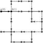
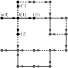
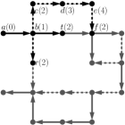
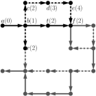
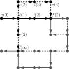
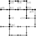
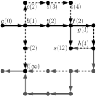
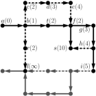
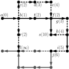
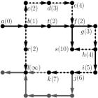
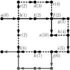
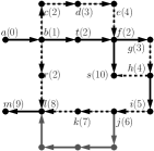
Figure 3: A computation of an optimal walk w.r.t. the penalized weight from $a$ to $m$ in $G$. Numbers represent the distance from the start $a$. Black vertices are reached or scanned and black edges were relaxed. Dotted edges represent maneuver edges. Steps 6 and 7 are depicted in the same figure (they are equal), analogously for steps 8 and 9.

4 Conclusion

We have introduced a novel generic model of maneuvers that is able to capture almost arbitrarily complex route restrictions, traffic regulations and even some dynamic aspects of the route planning problem. It can model anything from single vertices to long self-intersecting walks as restricted, negative, positive or prohibited maneuvers. We have shown how to incorporate this model into Dijkstra’s algorithm so that no adjustment of the underlying road network graph is needed. The running time of the proposed Algorithm 1 is only marginally larger than that of ordinary Dijkstra’s algorithm (Theorem 3.1) in practical networks.

Our algorithm can be relatively straightforwardly extended to a bidirectional algorithm by running it simultaneously from the start vertex in the original network and from the target vertex in the reversed network. A termination condition must reflect the fact that chained contexts of vertex-context pairs scanned in both directions might contain maneuvers as subwalks. Furthermore, since the A* algorithm is just an ordinary Dijkstra’s algorithm with edge weights adjusted by a potential function, our extension remains correct for A* if the road network is proper (Definition 4, namely iii.) even with respect to this potential function.

Finally, we would like to highlight that, under reasonable assumptions, our model can be incorporated into many established route planning approaches.

References

- [1] J. Anez, T. De La Barra, and B. Perez. Dual graph representation of transport networks. Transportation Research Part B: Methodological, 30(3):209 – 216, 1996.
- [2] B. Cherkassky, A. V. Goldberg, and T. Radzik. Shortest paths algorithms: Theory and experimental evaluation. Mathematical Programming, 73(2):129–174, 1996.
- [3] D. Delling, P. Sanders, D. Schultes, and D. Wagner. Engineering route planning algorithms. In Algorithmics of Large and Complex Networks. Lecture Notes in Computer Science, pages 117–139, Berlin, Heidelberg, 2009. Springer.
- [4] E. Dijkstra. A note on two problems in connexion with graphs. Numerische Mathematik, 1:269–271, 1959.
- [5] E. Gutierrez and A. Medaglia. Labeling algorithm for the shortest path problem with turn prohibitions with application to large-scale road networks. Annals of Operations Research, 157:169–182, 2008. 10.1007/s10479-007-0198-9.
- [6] P. E. Hart, N. J. Nilsson, and B. Raphael. Correction to “A formal basis for the heuristic determination of minimum cost paths”. SIGART, 1(37):28–29, 1972.
- [7] P. Hlineny and O. Moris. Scope-Based Route Planning. In ESA’11: Proceedings of the 19th conference on Annual European Symposium, pages 445–456, Berlin Heidelberg, 2011. Springer-Verlag. arXiv:1101.3182 (preprint).
- [8] J. Jiang, G. Han, and J. Chen. Modeling turning restrictions in traffic network for vehicle navigation system. In Proceedings of the Symposium on Geospatial Theory, Processing, and Applications., 2002.
- [9] R. F. Kirby and R. B. Potts. The minimum route problem for networks with turn penalties and prohibitions. Transportation Research, 3:397–408, 1969.
- [10] S. Pallottino and M. G. Scutella. Shortest path algorithms in transportation models: classical and innovative aspects. Technical report, Univ. of Pisa, 1997.
- [11] I. S. Pohl. Bi-directional and heuristic search in path problems. PhD thesis, Stanford University, Stanford, CA, USA, 1969.
- [12] D. Schultes. Route Planning in Road Networks. PhD thesis, Karlsruhe University, Karlsruhe, Germany, 2008.
- [13] D. Villeneuve and G. Desaulniers. The shortest path problem with forbidden paths. European Journal of Operational Research, 165(1):97 – 107, 2005.
- [14] S. Winter. Modeling costs of turns in route planning. GeoInformatica, 6:345–361, 2002. 10.1023/A:1020853410145.
- [15] A. K. Ziliaskopoulos and H. S. Mahmassani. A note on least time path computation considering delays and prohibitions for intersection movements. Transportation Research Part B: Methodological, 30(5):359 – 367, 1996.