Reduction of mean-square advection in turbulent passive scalar mixing

Abstract

Direct numerical simulation data shows that the variance of the coupling term in passive scalar advection by a random velocity field is smaller than it would be if the velocity and scalar fields were statistically independent. This effect is analogous to the ‘depression of nonlinearity’ in hydrodynamic turbulence. We show that the trends observed in the numerical data are qualitatively consistent with the predictions of closure theories related to Kraichnan’s Direct Interaction Approximation. The phenomenon is demonstrated over a range of Prandtl numbers. In the inertial-convective range the depletion is approximately constant with respect to wavenumber. The effect is weaker in the Batchelor range.

I introduction

The modal amplitudes in the Fourier decomposition of any homogeneous random field are uncorrelated. In a Gaussian random field, they are also statistically independent; but in homogeneous turbulence, nonlinearity produces statistical dependence among the amplitudes. The simplest consequence is that the third-order correlations representing energy transfer, which would vanish in a Gaussian random field, do not vanish in homogeneous turbulence.

Some further consequences of statistical dependence of Fourier amplitudes in homogeneous turbulence were considered in an important paper by Chen, Herring, Kerr and Kraichnan,[1] which compared various fourth-order moments with the corresponding moments in a Gaussian random field with the same second-order properties as the turbulent velocity field (the construction of such Gaussian surrogates is sometimes called ‘kinematic simulation’ [2, 3]). Among the quantities investigated by Chen et al. was the variance of the fluctuating nonlinear term in the Navier-Stokes equations,

$$\langle\left|{\bm{u}(\bm{x},t)}\cdot\nabla{\bm{u}(\bm{x},t)}+\nabla p(\bm{x},t)\right|^{2}\rangle.$$ (1)

It had been observed [4] that this quantity is significantly smaller in a turbulent velocity field than in its Gaussian counterpart; that is, there is a significant (negative) cumulant contribution to the fourth order moment defined by Eq. (1). One of the mechanisms which can lead to this depression of nonlinearity is the preferential alignment of velocity and vorticity, also called Beltramization.[5] However, this preferential alignment is not the only non-trivial mechanism which is consistent with the depression of nonlinearity; we will return to this issue in Section V.

From the viewpoint of a Fourier analysis of the spectrum of the correlation in Eq. (1), the depression of nonlinearity is a consequence of statistical dependence of the uncorrelated Fourier amplitudes that enter the expression for this spectrum. One finding of Chen et al. was that this phenomenon appears to be well predicted by Kraichnan’s [6] Direct Interaction Approximation (DIA). The successful prediction of a nonzero fourth-order cumulant by a closure theory might seem unexpected or even surprising, since from the very beginning, closure theories have been associated with cumulant discard hypotheses;[7] the debate between Kraichnan and Proudman at the famous 1961 Marseille conference [8] centered on this issue.[24] The computation of a nonzero cumulant and the favorable comparison with data perhaps vindicate, somewhat after the fact, Kraichnan’s assertion at that time,[9] that DIA does not assume (or imply) the vanishing of fourth order cumulants.

In the present work we will show that an effect of statistical dependence of Fourier amplitudes analogous to depression of nonlinearity also appears in the advection of a passive scalar $\theta$. Thus, we consider the scalar analog of the moment in Eq. (1): the variance of fluctuations of the bilinear scalar-velocity coupling

$$\langle({\bm{u}}({\bm{x}},t)\cdot\nabla\theta({\bm{x}},t))^{2}\rangle.$$ (2)

Herring and Métais [10] have shown that this quantity is smaller in passive scalar advection than it would be if the Fourier amplitudes of velocity and scalar were statistically independent, even at the more refined level of Fourier spectra. We confirm their conclusions using higher resolution DNS data, and following Chen et al., show that closures related to the DIA predict trends consistent with the data.

A different perspective on non-Gaussian properties of turbulence is provided by recent detailed studies of the properties of realizations of turbulent velocity fields. Such studies, made possible by high resolution direct numerical simulations,[11] reveal the existence of flow structures such as vortex tubes and sheets, and spotty regions of very high dissipation; in comparison, since a Gaussian random field is simply space- and time-filtered white noise, it is expected to be essentially ‘featureless.’ This viewpoint makes the existence of such structures the most significant effect of non-Gaussianity in turbulence. In the present paper we focus on a statistical characterization of non-Gaussian features in turbulence and do not investigate features of the instantaneous flow realizations. We suggest, however, that investigating the connections between this physical space perspective and the viewpoint of dependence among Fourier modes can be a useful direction for future research.

The paper is organized as follows: in Section II the theoretical considerations leading to closure expressions for the mean-square advection term are given. Section III presents details of the numerical evaluation of cumulant corrections. Section IV presents comparisons between closure computations and direct numerical simulation data. Section V contains a discussion of the results. Conclusions are drawn in Section VI.

II analysis

We consider the advection of a passive scalar in homogeneous turbulence. The governing equation is

$$\left[\partial_{t}+\alpha k^{2}\right]\theta(\bm{k},t)=-ik_{i}\int d{\bm{p}}d{\bm{q}}\ \delta({\bm{k}-\bm{p}-\bm{q}})\theta({\bm{p}},t)u_{i}({\bm{q}},t)+f_{\theta}(\bm{k},t),$$ (3)

where $\alpha$ denotes the scalar diffusivity, and $f_{\theta}({\bm{k}},t)$ is a source of scalar fluctuations that we will assume confined to the large scales. By analogy to Chen et al., we consider the contribution of each Fourier mode to the variance of the velocity-scalar coupling term. It is defined by

$$W_{\theta}({\bm{k}},t)=k_{i}k_{j}\int d{\bm{p}}\ d{\bm{q}}\ \int d{\bm{p}}^{\prime}\ d{\bm{q}}^{\prime}\ \delta({\bm{k}-\bm{p}-\bm{q}})\delta({\bm{k}+\bm{p}^{\prime}+\bm{q}^{\prime}})\langle\theta({\bm{p}},t)u_{i}({\bm{q}},t)\theta({\bm{p}}^{\prime},t)u_{j}({\bm{q}}^{\prime},t)\rangle$$

(4)

The integral of $W_{\theta}({\bm{k}},t)$ over all wavevectors is equal to the moment in Eq. (2),

$$\int d{\bm{k}}\ W_{\theta}({\bm{k}},t)=\langle[\bm{u}({\bm{x}},t)\cdot\nabla\theta({\bm{x}},t)]^{2}\rangle.$$ (5)

Without introducing any assumptions, we can write

$$W_{\theta}({\bm{k}},t)=W_{\theta}^{G}({\bm{k}},t)+W_{\theta}^{C}({\bm{k}},t),$$ (6)

where $W_{\theta}^{G}({\bm{k}},t)$ is evaluated assuming the independence of the Fourier amplitudes in Eq. (4) and $W_{\theta}^{C}({\bm{k}},t)$ is a cumulant correction. In the following we will consider the isotropic case. In that case the velocity and scalar are uncorrelated. Then

$$W_{\theta}^{G}({\bm{k}},t)=k_{i}k_{j}\int d{\bm{p}}\ d{\bm{q}}\ \delta({\bm{k}-\bm{p}-\bm{q}})\ U_{\theta}({\bm{p}},t)U_{ij}({\bm{q}},t),$$ (7)

where

$$U_{ij}({\bm{k}},t)=\langle u_{i}({\bm{k}},t)u_{j}(-{\bm{k}},t)\rangle$$ (8)

is the single-time velocity autocorrelation and

$$U_{\theta}({\bm{k}},t)=\langle\theta({\bm{k}},t)\theta(-{\bm{k}},t)\rangle$$ (9)

is the single-time scalar autocorrelation.

We now analyze $W_{\theta}$ using Kraichnan’s DIA theory. There are many equivalent formulations of this theory, but for this analysis, the Langevin model formulation [12] is the most convenient. The DIA Langevin model for passive scalar advection replaces the exact governing equation Eq. (3) by

$$\left[\partial_{t}+\alpha k^{2}\right]\theta(\bm{k},t)+\int^{t}_{0}ds\ \eta_{\theta}(\bm{k};t,s)\theta(\bm{k},s)=-ik_{i}\int d{\bm{p}}d{\bm{q}}\ \delta({\bm{k}-\bm{p}-\bm{q}})\xi_{\theta}({\bm{p}},t)\xi_{i}({\bm{q}},t)+f_{\theta}(\bm{k},t),$$ (10)

where $\xi_{\theta}$ and $\xi_{i}$ are independent Gaussian random variables with the same two-time correlation functions as $\theta$ and $u_{i}$:

$$\langle\xi_{\theta}({\bm{k}},t)\xi_{\theta}(-{\bm{k}},t^{\prime})\rangle=\langle\theta({\bm{k}},t)\theta(-{\bm{k}},t^{\prime})\rangle=U_{\theta}({\bm{k}};t,t^{\prime})$$ (11)

$$\langle\xi_{i}({\bm{k}},t)\xi_{j}(-{\bm{k}},t^{\prime})\rangle=\langle u_{i}({\bm{k}},t)u_{j}(-{\bm{k}},t^{\prime})\rangle=U_{ij}({\bm{k}};t,t^{\prime})$$ (12)

and the damping function $\eta_{\theta}$ is defined as

$$\eta_{\theta}({\bm{k}};t,t^{\prime})=k_{i}k_{j}\int d{\bm{p}}\ d{\bm{q}}\ \delta({\bm{k}-\bm{p}-\bm{q}})\ G_{\theta}({\bm{p}};t,t^{\prime})U_{ij}({\bm{q}};t,t^{\prime}).$$ (13)

Here, $G_{\theta}$ is the response function, defined as the inverse of the (formally) linear operator on the left side of Eq. (10). This linearity allows us to write, ignoring the contribution of the scalar source term,

$$\theta({\bm{k}},t)=-ik_{i}\int^{t}_{0}ds\ G_{\theta}({\bm{k}};t,s)\int d{\bm{p}}d{\bm{q}}\ \delta({\bm{k}-\bm{p}-\bm{q}})\xi_{\theta}({\bm{p}},s)\xi_{i}({\bm{q}},s).$$ (14)

This brings up an important feature of DIA, namely that it is not closed in terms of the correlation function alone. The introduction of the response function is one major contribution of DIA to turbulence theory.[25] DIA provides equations of motion for both $G_{\theta}$ and the correlation function $U_{\theta}$ related to the model Eq. (10). We refer to [13] for details.

Paraphrasing Kraichnan’s own description of DIA, we see that it first replaces the nonlinear coupling by a random forcing by surrogate statistically independent random fields with the same second-order properties as the actual fields; this step suppresses any statistical dependence among Fourier modes that develops under the exact evolution. These correlations are then modeled by the damping provided by $\eta_{\theta}$; then the transfer of scalar fluctuations between modes is treated in DIA as the result of this damping acting against the forcing. Perhaps the most important qualitative feature to note is that the theory requires two-time statistics: this complication is inevitable given that DIA attempts to describe complex bilinear interactions by means of second-order statistics alone.

Thus, DIA can be described as the replacement

$$-ik_{i}\int d{\bm{p}}d{\bm{q}}\ \delta({\bm{k}-\bm{p}-\bm{q}})\theta({\bm{p}},t)u_{i}({\bm{q}},t)\rightarrow-\left[\int^{t}_{0}ds\ \eta_{\theta}(\bm{k};t,s)\theta(\bm{k},s)\right.$$

$$\left.+ik_{i}\int d{\bm{p}}d{\bm{q}}\ \delta({\bm{k}-\bm{p}-\bm{q}})\xi_{\theta}({\bm{p}},t)\xi_{i}({\bm{q}},t)\right],$$ (15)

where the arrow simply indicates modeling; at this point, there is no assertion about an ‘approximation.’ Then the DIA model for the variance of the advection term is the variance of the right side of Eq. (15):

$$\left\langle\left|\int^{t}_{0}ds\ \eta_{\theta}(\bm{k};t,s)\theta(\bm{k},s)+ik_{i}\int d{\bm{p}}d{\bm{q}}\ \delta({\bm{k}-\bm{p}-\bm{q}})\xi_{\theta}({\bm{p}},t)\xi_{i}({\bm{q}},t)\right|^{2}\right\rangle$$

$$=\int^{t}_{0}ds\int^{t}_{0}ds^{\prime}\ \eta_{\theta}(\bm{k};t,s)\eta_{\theta}(\bm{k};t,s^{\prime})\langle\theta(\bm{k},s)\theta(-\bm{k},s^{\prime})\rangle$$ (16)

$$-2ik_{i}\int d{\bm{p}}d{\bm{q}}\ \delta({\bm{k}-\bm{p}-\bm{q}})\int^{t}_{0}ds\ \eta_{\theta}(\bm{k};t,s)\left\langle\xi_{\theta}(-{\bm{p}},t)\xi_{i}(-{\bm{q}},t)\theta(\bm{k},s)\right\rangle$$ (17)

$$+k_{i}k_{j}\int d{\bm{p}}d{\bm{q}}\ \int d{\bm{p}}^{\prime}d{\bm{q}}^{\prime}\ \delta({\bm{k}-\bm{p}-\bm{q}})\delta({\bm{k}-\bm{p}^{\prime}-\bm{q}^{\prime}})\langle\xi_{\theta}({\bm{p}},t)\xi_{i}({\bm{q}},t)\xi_{\theta}(-{\bm{p}}^{\prime},t)\xi_{j}(-{\bm{q}}^{\prime},t)\rangle.$$ (18)

The rules for correlations of Gaussian variables, and the relations Eqs. (11) and (12) give for the term in Eq. (18),

$$k_{i}k_{j}\int d{\bm{p}}d{\bm{q}}\ \int d{\bm{p}}^{\prime}d{\bm{q}}^{\prime}\ \delta({\bm{k}-\bm{p}-\bm{q}})\delta(-{\bm{k}-\bm{p}^{\prime}-\bm{q}^{\prime}})\langle\xi_{\theta}({\bm{p}},t)\xi_{i}({\bm{q}},t)\xi_{\theta}({\bm{p}}^{\prime},t)\xi_{i}({\bm{q}}^{\prime},t)\rangle$$

$$=k_{i}k_{j}\int d{\bm{p}}d{\bm{q}}\ \delta({\bm{k}-\bm{p}-\bm{q}})U_{\theta}({\bm{p}},t)U_{ij}({\bm{q}},t)=W_{\theta}^{G}({\bm{k}},t),$$ (19)

so that, as was evident from its definition, this term simply reproduces the Gaussian contribution Eq. (7). The remaining terms are cumulant corrections. Obviously, the term in Eq. (16) is simply

$$\int^{t}_{0}ds\int^{t}_{0}ds^{\prime}\ \eta_{\theta}(\bm{k};t,s)\eta_{\theta}(\bm{k};t,s^{\prime})\langle\theta(\bm{k},s)\theta(-\bm{k},s^{\prime})\rangle$$

$$=k_{i}k_{j}k_{m}k_{n}\int^{t}_{0}ds\int^{t}_{0}ds^{\prime}\ \int d{\bm{p}}\ d{\bm{q}}\ \delta({\bm{k}-\bm{p}-\bm{q}})\ \int d{\bm{p}}^{\prime}\ d{\bm{q}}^{\prime}\ \delta({\bm{k}-\bm{p}^{\prime}-\bm{q}^{\prime}})\ \times$$

$$G_{\theta}({\bm{p}};t,s)U_{ij}({\bm{q}};t,s)G_{\theta}({\bm{p}}^{\prime};t,s^{\prime})U_{mn}({\bm{q}}^{\prime};t,s^{\prime})U_{\theta}({\bm{k}};s,s^{\prime}),$$ (20)

where we have used the definition Eq. (13) of $\eta_{\theta}$.

The term in Eq. (17) is evaluated by expressing $\theta$ in terms of the $\xi_{\theta}$ and $\xi_{i}$ using Eq. (14), so that

$$-2ik_{i}\int d{\bm{p}}d{\bm{q}}\ \delta({\bm{k}-\bm{p}-\bm{q}})\int^{t}_{0}ds\ \eta_{\theta}(\bm{k};t,s)\left\langle\xi_{\theta}(-{\bm{p}},t)\xi_{i}(-{\bm{q}},t)\theta(\bm{k},s)\right\rangle$$

$$=-2ik_{i}(-ik_{j})\int d{\bm{p}}d{\bm{q}}\ \int d{\bm{p}}^{\prime\prime}d{\bm{q}}^{\prime\prime}\ \delta({\bm{k}-\bm{p}-\bm{q}})\delta({\bm{k}-\bm{p}^{\prime\prime}-\bm{q}^{\prime\prime}})\int^{t}_{0}ds\ \int^{s}_{0}ds^{\prime}\ \eta_{\theta}(\bm{k};t,s)G_{\theta}({\bm{k}};s,s^{\prime})\times$$

$$\left\langle\xi_{\theta}(-{\bm{p}},t)\xi_{i}(-{\bm{q}},t)\xi_{\theta}({\bm{p}}^{\prime\prime},s^{\prime})\xi_{j}({\bm{q}}^{\prime\prime},s^{\prime})\right\rangle$$

$$=-2k_{i}k_{j}k_{m}k_{n}\int d{\bm{p}}d{\bm{q}}\ \int d{\bm{p}}^{\prime}d{\bm{q}}^{\prime}\ \delta({\bm{k}-\bm{p}-\bm{q}})\delta({\bm{k}-\bm{p}^{\prime}-\bm{q}^{\prime}})\int^{t}_{0}ds\ \int^{s}_{0}ds^{\prime}\ \times$$

$$G_{\theta}({\bm{p}}^{\prime};t,s)U_{mn}({\bm{q}}^{\prime};t,s)G_{\theta}({\bm{k}};s,s^{\prime})U_{\theta}({\bm{p}};t,s^{\prime})U_{ij}({\bm{q}};t,s^{\prime}).$$ (21)

The cumulant contribution $W^{C}_{\theta}$ is the sum of the results of Eqs. (20) and (21). But to express the result in the most transparent form, it will be useful to reformulate Eq. (20) somewhat: abbreviating the integrand for simplicity,

$$\int^{t}_{0}ds\int^{t}_{0}ds^{\prime}\ {\cal I}({\bm{p},\bm{q},\bm{p}^{\prime},\bm{q}^{\prime}};t,s,s^{\prime})=\left(\int^{t}_{0}ds\int^{s}_{0}ds^{\prime}\ +\int^{t}_{0}ds\int^{t}_{s}ds^{\prime}\ \right){\cal I}({\bm{p},\bm{q},\bm{p}^{\prime},\bm{q}^{\prime}};t,s,s^{\prime})$$

$$=\left(\int^{t}_{0}ds\int^{s}_{0}ds^{\prime}\ +\int^{t}_{0}ds^{\prime}\int^{s^{\prime}}_{0}ds\ \right){\cal I}({\bm{p},\bm{q},\bm{p}^{\prime},\bm{q}^{\prime}};t,s,s^{\prime}),$$ (22)

where the order of integration has been interchanged in the second term. Since the integrand is invariant under the simultaneous interchanges of $s$, $s^{\prime}$ and ${\bm{p}}$, ${\bm{p}}^{\prime}$, we obviously have

$$\int^{t}_{0}ds\int^{t}_{0}ds^{\prime}\ {\cal I}({\bm{p},\bm{q},\bm{p}^{\prime},\bm{q}^{\prime}};t,s,s^{\prime})=2\int^{t}_{0}ds\int^{s}_{0}ds^{\prime}\ {\cal I}({\bm{p},\bm{q},\bm{p}^{\prime},\bm{q}^{\prime}};t,s,s^{\prime}),$$ (23)

so we can write

$$\int^{t}_{0}ds\int^{t}_{0}ds^{\prime}\ \eta_{\theta}(\bm{k};t,s)\eta_{\theta}(\bm{k};t,s^{\prime})\langle\theta(\bm{k},s)\theta(-\bm{k},s^{\prime})\rangle$$

$$=2k_{i}k_{j}k_{m}k_{n}\int^{t}_{0}ds\int^{s}_{0}ds^{\prime}\ \int d{\bm{p}}\ d{\bm{q}}\ \delta({\bm{k}-\bm{p}-\bm{q}})\ \int d{\bm{p}}^{\prime}\ d{\bm{q}}^{\prime}\ \delta({\bm{k}-\bm{p}^{\prime}-\bm{q}^{\prime}})\ \times$$

$$G_{\theta}({\bm{p}};t,s)U_{ij}({\bm{q}};t,s)G_{\theta}({\bm{p}}^{\prime};t,s^{\prime})U_{mn}({\bm{q}}^{\prime};t,s^{\prime})U_{\theta}({\bm{k}};s,s^{\prime}).$$ (24)

Interchanging indices $(ij)$ and $(mn)$ and the wavevector arguments $({\bm{p},\bm{q}})$ and $({\bm{p}^{\prime},\bm{q}^{\prime}})$ and adding the result of Eq. (21), we obtain

$$W^{C}_{\theta}({\bm{k}},t)=-2k_{i}k_{j}k_{m}k_{n}\int d{\bm{p}}\ d{\bm{q}}\ \int d{\bm{p}}^{\prime}\ d{\bm{q}}^{\prime}\ \delta({\bm{k}-\bm{p}-\bm{q}})\delta({\bm{k}-\bm{p}^{\prime}-\bm{q}^{\prime}})\times$$

$$\int^{t}_{0}ds\ \int^{s}_{0}ds^{\prime}\ U_{ij}({\bm{q}};t,s)U_{mn}({\bm{q}}^{\prime};t,s^{\prime})\times$$

$$\left[G_{\theta}({\bm{p}};t,s)G_{\theta}({\bm{p}}^{\prime};t,s^{\prime})U_{\theta}({\bm{k}};s,s^{\prime})-G_{\theta}({\bm{p}}^{\prime};t,s)G_{\theta}({\bm{k}};s,s^{\prime})U_{\theta}({\bm{p}};t,s^{\prime})\right].$$ (25)

This expression makes clear an important property of the DIA cumulant correction, namely that it vanishes identically, independently of the velocity field, in the scalar non-diffusive truncated ensemble when diffusivity $\alpha=0$ and a maximum wavenumber is imposed on the scalar fluctuations. This equilibrium ensemble is Gaussian, therefore all cumulants vanish. The proof follows from the properties of this system, that the scalar field is in steady-state equipartition, so that $U_{\theta}({\bm{k}},t)$ is a constant, and the fluctuation-dissipation relation

$$U_{\theta}({\bm{k}};t,t^{\prime})=U_{\theta}({\bm{k}})[G_{\theta}({\bm{k}};t,t^{\prime})+G_{\theta}({\bm{k}};t^{\prime},t)]$$ (26)

holds. (Note that the response function is causal: $G_{\theta}({\bm{k}};t,t^{\prime})=0$ for $t^{\prime}>t$.) Substituting these relations in Eq. (25) shows at once that $W^{C}_{\theta}\equiv 0$ independently of the velocity field, as required. We remark that this conclusion is a nontrivial check of the DIA calculation, since DIA only treats moments, and the multipoint probability density functions play no explicit role.

It is easily verified that the same result holds for the cumulant corrections to the mean-square nonlinearity in the analysis of the velocity field.[1]

III numerical evaluation of the DIA cumulant corrections

At this point, we introduce the assumption that the velocity field is time stationary and that the scalar field is maintained in a steady state by a scalar source term. Then numerical evaluation is greatly simplified by expressing the results in terms of spectra rather than correlations. If $W_{\theta}({\bm{k}})$ depends only on $k=|\bm{k}|$, then the corresponding spectrum is

$$w_{\theta}(k)=\oint dS({\bm{k}})\ W_{\theta}({\bm{k}})=4\pi k^{2}W_{\theta}(k)$$ (27)

and, corresponding to Eq. (6), we have

$$w_{\theta}(k)=w_{\theta}^{G}(k)+w_{\theta}^{C}(k).$$ (28)

We introduce the usual energy and scalar fluctuation spectra by

$$U_{ij}({\bm{k}})=\frac{1}{4\pi k^{2}}E(k)(\delta_{ij}-k^{-2}k_{i}k_{j})\quad U_{\theta}({\bm{k}})=\frac{1}{2\pi k^{2}}E_{\theta}(k).$$ (29)

With these simplifications, Eq. (7) can be reformulated, following procedures that are standard in the closure literature, as

$$w_{\theta}^{G}(k)=k^{3}\int_{\Delta}(1-z^{2})E(p)E_{\theta}(q)\frac{dp}{p}\frac{dq}{q}.$$ (30)

where, as usual, the integration region $\Delta$ indicates that the wavenumbers $k,p,q$ are the sides of a triangle and $z$ is the cosine of the angle between the sides of lengths $k$ and $p$. The time integrations in Eq. (25) are evaluated by replacing the two-time quantities by functions of time difference only, then passing to the steady state limit $t\rightarrow\infty$. Since we wanted to be able to compute the cumulants under a variety of conditions, we found it expedient to make the double time integrations of Eq. (25) analytically computable by assuming simple exponential time-dependence

$$G_{\theta}({\bm{k}};t-t^{\prime})=e^{-\eta_{\theta}(k)(t-t^{\prime})}H(t-t^{\prime}),\quad U_{\theta}({\bm{k}};t-t^{\prime})=U_{\theta}({\bm{k}})e^{-\eta_{\theta}(k)|t-t^{\prime}|},$$

$$\quad U_{ij}({\bm{k}};t-t^{\prime})=U_{ij}({\bm{k}})e^{-\eta_{\theta}(k)|t-t^{\prime}|}.$$ (31)

As usual, $H(s)$ is the ‘Heaviside function’ equal to one for $s>0$ and zero otherwise; we have also introduced a ‘fluctuation-dissipation’ relation in which the damping function $\eta_{\theta}$ is the same in the scalar response function $G_{\theta}$ and two-time correlation function $U_{\theta}$. The very commonly introduced exponential ansatz for the two-time dependence is also made by Herring and Métais; we emphasize that we use it entirely in the interest of analytical simplicity, and no assertion is made that it approximates the two-time response that would actually be predicted by DIA. But since two-time statistics enter our results only after integration over all time-differences, any resulting errors are unlikely to be qualitatively important.

After making all of these simplifications, the cumulant spectrum is evaluated as

$$w_{\theta}^{C}(k)=\frac{1}{2}\int_{\Delta}\frac{dp}{p}\frac{dq}{q}\int_{\Delta^{\prime}}\frac{dp^{\prime}}{p^{\prime}}\frac{dq^{\prime}}{q^{\prime}}(1-z^{2})kq^{2}E(p)(1-z^{\prime 2})kq^{\prime 2}E(p^{\prime})\times$$

$$\left[\left(\Xi_{kpqp^{\prime}q^{\prime}}+\Xi_{kp^{\prime}q^{\prime}pq}\right)E_{\theta}(k)-2\Xi_{kpqp^{\prime}q^{\prime}}(k/q)^{2}E_{\theta}(q)\right],$$ (32)

where $\Delta^{\prime}$ indicates that the wavenumbers $k,p^{\prime},q^{\prime}$ are the sides of a triangle, $z^{\prime}$ is the cosine of the angle between the sides of lengths $k$ and $p^{\prime}$, and the time integrals yield

$$\Xi_{kpqp^{\prime}q^{\prime}}=\frac{1}{\eta_{\theta}(k)+{\eta}(p^{\prime})+{\eta}_{\theta}(q^{\prime})}~{}\frac{1}{\eta(p)+\eta_{\theta}(q)+\eta(p^{\prime})+\eta_{\theta}(q^{\prime})}.$$ (33)

The spectra $E(k)$ and $E_{\theta}(k)$ are evaluated using EDQNM (Eddy-Damped Quasi-Normal Markovian) closures [14, 15]

$$\left[\frac{\partial}{\partial t}+2\nu k^{2}\right]E(k)=\int_{\Delta}\Theta(k,p,q)~{}[xy+z^{3}]pE(q)\left[k^{2}E(p)-p^{2}E(k)\right]\frac{dpdq}{pq}+F(k)$$ (34)

$$\left[\frac{\partial}{\partial t}+2\alpha k^{2}\right]E_{\theta}(k)=\int_{\Delta}\Theta^{\theta}(k,p,q)~{}[1-y^{2}]kE(q)\left[k^{2}E_{\theta}(p)-p^{2}E_{\theta}(k)\right]\frac{dpdq}{pq}+F_{\theta}(k),$$ (35)

in which $F(k)$ and $F_{\theta}(k)$ are external forcing terms confined to the smallest wavenumbers (Both $F(k)$ and $F_{\theta}(k)$ are unity for $k\leq 2$ and zero elsewhere), $x$ is the cosine of the angle between the sides of lengths $p$ and $q$, and $y$ is the cosine of the angle between the sides of lengths $k$ and $q$. The triad relaxation times $\Theta(k,p,q)$ and $\Theta^{\theta}(k,p,q)$ are

$$\Theta=\frac{1}{\eta(k)+\eta(p)+\eta(q)},\qquad\Theta^{\theta}=\frac{1}{\eta_{\theta}(k)+\eta(p)+\eta_{\theta}(q)}.$$ (36)

We use the (inverse) time-scales

$$\eta(k)=\lambda\sqrt{\int_{0}^{k}E(r)dr}+\nu k^{2},\qquad\eta_{\theta}(k)=\lambda_{\theta}\sqrt{\int_{0}^{k}E(r)dr}+\alpha k^{2}$$ (37)

and we set the constants $\lambda=\lambda_{\theta}=0.5$. Note that $\eta$ and $\eta_{\theta}$ are the same quantities that appear in Eq. (31). An interesting perspective for future work would be the use of a Lagrangian two-time theory [16, 17] or a self-consistent Markovian closure [18, 19] to evaluate the cumulants, which would avoid the introduction of adjustable constants and ad-hoc formulation of damping time-scales. Computations are carried out on a logarithmically spaced grid with $36$ gridpoints per octave and results are evaluated when a steady state is reached.

IV numerical comparisons

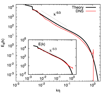
Figure 1: DNS and theoretical results for the scalar spectra in isotropic turbulence at a Taylor-scale Reynolds number of $427$ and ${\mathcal{P}r}=1$. In the inset the energy spectra are shown.

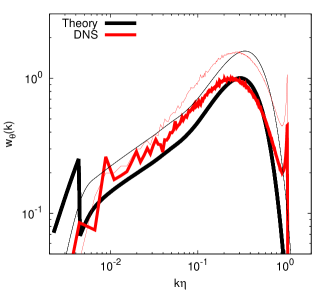
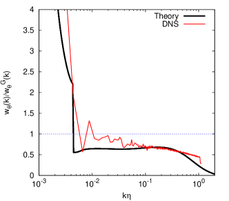
Figure 2: DNS and theoretical results in isotropic turbulence at a Taylor-scale Reynolds number of $427$ and ${\mathcal{P}r}=1$. Left: spectrum of the mean square advection term of the scalar equation in isotropic turbulence. Also shown are the Gaussian spectra (thin lines). Right: ratio of the spectra to the Gaussian spectra.

In this section, we confirm the reduction of mean-square advection in DNS data,[10] and compare the results with closure predictions. We have computed the scalar spectrum and energy spectrum by closure theory as described in the previous section and the parameters have been chosen to match the DNS as closely as possible. The DNS database used is from high resolution ($1024^{3}$ gridpoint) pseudospectral direct numerical simulations of a passive scalar advected by isotropic turbulence;[20]. The force terms for the velocity and scalar fluctuations are random-Gaussian and delta-correlated in time (and solenoidal for the velocity forcing), acting in the wave-number range $1\leq k\leq 2$. In these simulations the Reynolds number based on the Taylor microscale is equal to $427$ and the Prandtl number ${\mathcal{P}r}=\nu/\alpha=1$. The resolution is higher than that used in the simulations of both Herring and Métais[10] and Chen et al.[1].

Using DNS data, $w_{\theta}(k)$ can be determined from Eqs. (4) and (27). The contribution $w_{\theta}^{G}(k)$ is obtained by randomizing the phases of the Fourier amplitudes of $\theta(\bm{x},t)$; this randomization will yield scalar fields with statistically independent Fourier amplitudes without changing the wavenumber spectra. This independence, not the probability density function itself, is the key property for us. The fields are therefore random-phase fields and the amplitude statistics are not necessarily Gaussian.

Figure 1 compares the scalar variance spectra in DNS and the closure computations at $R_{\lambda}=427$ and ${\mathcal{P}r}=1$. The inset shows the energy spectra. The wavenumber of these results is normalized by the Kolmogorov scale, which is equal to the Batchelor scale for unit Prandtl number. Good agreement is observed between the DNS results and the EDQNM results. A Corrsin-Obukhov inertial range for the scalar spectrum and a Kolmogorov inertial range for the energy spectrum, both approximately proportional to $k^{-5/3}$ are clearly observed.

In Figure 2, left, the spectrum of the advection term $w_{\theta}(k)$ is shown, as well as its Gaussian estimate. These spectra, for both closure and DNS, display an increasing trend in the inertial range and peak around the Batchelor scale. The peak of $w_{\theta}(k)$ is smaller then the Gaussian value, which indicates a reduction of mean-square advection. This reduction is more clearly observed in Figure 2, right, in which we display the measure of the departure from Gaussianity, the ratio $w_{\theta}(k)/w_{\theta}^{G}(k)$ [10]; the analogous quantity for the velocity field was introduced by Kraichnan and Panda.[4] The ratio departs noticeably from the Gaussian values over the entire wavenumber range, and a significant depression of the $w_{\theta}(k)$ compared to the Gaussian value is observed at scales larger than the forcing scales. The region where $w_{\theta}(k)/w_{\theta}^{G}(k)<1$ extends over the entire inertial-convective range. These general trends, including the observation that $w_{\theta}(k)/w_{\theta}^{G}(k)>1$ at large scales, are consistent with previous observations.[1, 10]. The results in Figures 1 and 2 show that the closure yields results in good agreement with the DNS results.

The ratio of the measured variance to the value assuming independence of the Fourier amplitudes,

$$\rho_{\theta}=\frac{\langle({\bm{u}}\cdot\nabla\theta)^{2}\rangle}{\langle|{\bm{u}}|^{2}\rangle\langle|\nabla\theta|^{2}\rangle}=\frac{\displaystyle\int^{\infty}_{0}w_{\theta}(k)dk}{\displaystyle\int^{\infty}_{0}w^{G}_{\theta}(k)dk}$$ (38)

is also of interest. Figure 2 (left) shows that the spectrum $w_{\theta}(k)$ is an increasing function of the wavenumber, consequently its integral is dominated by the small scales, where the variance is reduced. The DNS value for $\rho_{\theta}$ is 0.41 and the closure value is 0.54. These values are consistent with the previous reported results: Herring and Métais[10] quotes a value for $\rho_{\theta}$ of about 0.5 in the scalar case, and Kraichnan and Panda [4] reported the value 0.57 for the comparable ratio of the mean-square nonlinearity. We conclude that the effect we investigate is observed in DNS and closure and is of comparable magnitude in both.

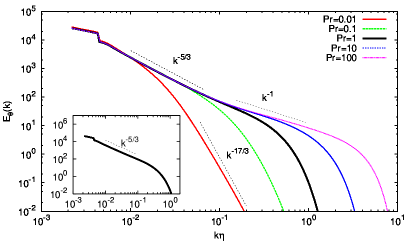
Figure 3: Closure results for the spectrum of the scalar variance at a Taylor-scale Reynolds number of $427$ and ${\mathcal{P}r}=0.01,..,100$. Inset: energy spectrum.

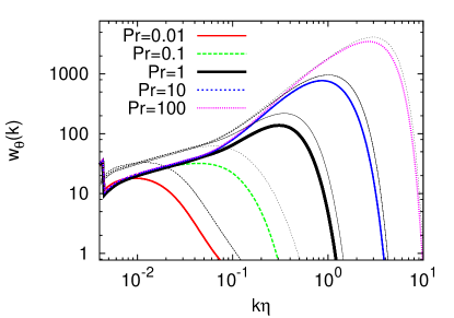
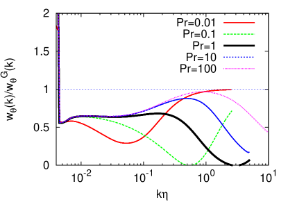
Figure 4: Closure results for the spectrum of the mean square advection term at a Taylor-scale Reynolds number of $427$ and ${\mathcal{P}r}=0.01,..,100$. Also shown are the Gaussian spectra (thin lines). Right: ratio of the spectra to the Gaussian spectra.

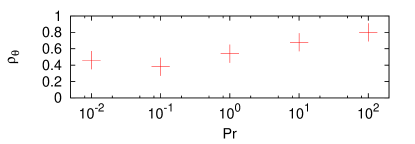
Figure 5: The mean square advection term of the scalar equation in isotropic turbulence compared to its Gaussian value as a function of the Prandtl number at a Taylor-scale Reynolds number of $427$.

In problems involving passive scalars, the dependence on Prandtl number is always of interest. We investigate the effect of the Prandtl number on the reduction of mean-square advection by varying the Prandtl number from $0.01$ to $100$ at a fixed Reynolds number $R_{\lambda}=427$. There is no DNS data available for these cases, in particular for the high Prandtl number cases, so we limit the discussion to closure predictions. Figures 3 and 4 show the closure results. In Figure 3 we show the scalar spectrum for five different Prandtl numbers. At low Prandtl numbers the $k^{-17/3}$ spectrum is observed and at large ${\mathcal{P}r}$ we observe a $k^{-1}$ spectrum [21, 22].

Figure 4 (left) shows the spectrum of the advection term. For all ${\mathcal{P}r}$, this spectrum is an increasing function of the wavenumber. At the highest value of ${\mathcal{P}r}$, the spectrum seems to approach its Gaussian estimate. Figure 4 (right) shows $w_{\theta}(k)/w_{\theta}^{G}(k)$. It is clearly observed that the spectrum is under its Gaussian value for all scales, except the forced scales, but the precise behavior seems to depend strongly on the Prandtl number. In the inertial-convective range the depletion is approximately constant with respect to wavenumber. The effect is weaker in the Batchelor range.

The numerical values of $\rho_{\theta}$ are displayed in Figure 5. The value ranges from a minimum of $\rho_{\theta}=0.38$ at ${\mathcal{P}r}=0.1$ to a maximum of $\rho_{\theta}=0.8$ at ${\mathcal{P}r}=100$. This change is non-negligible, but the trend is rather weak if we consider that ${\mathcal{P}r}$ changes over four orders of magnitude in our simulations. The reduction of advection seems thus an effect which is persistent, but becomes weaker for high values of the Prandtl number. Its amount is mainly determined by the precise behavior of the cumulant-spectrum around the scale where the spectrum $w_{\theta}(k)$ peaks.

V Discussion: mechanisms of the suppression of advection

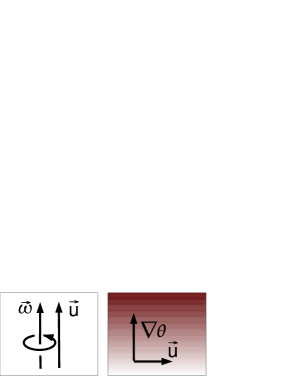
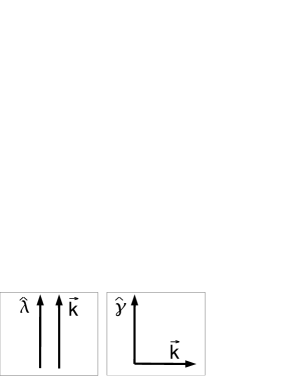
Figure 6: Left, top: velocity Beltramization; bottom: depression of nonlinearity through alignment of the Lamb-vector and the wavevector. Right: depletion of advection in physical and Fourier space. The scalar flux vector is defined as $\bm{\gamma}=\bm{u}\theta$.

The analysis of the variance of the nonlinear term in the Navier-Stokes equations by Chen et al.[1] was motivated in part by the suggestion of Levich and Tsinober [23] of the possibility of Beltramization, the preferential alignment of velocity and vorticity in turbulence. Since the nonlinear term can be written as

$$\nabla^{-2}\nabla\times\nabla\times(\bm{\omega}(\bm{x})\times\bm{u}(\bm{x})),$$ (39)

with $\bm{\omega}=\nabla\times\bm{u}$ the vorticity, this alignment will obviously reduce the magnitude of the nonlinear term, and hence will also reduce the intensity of its fluctuations, which is consistent with the observed depression of nonlinearity.

Another mechanism consistent with depression of nonlinearity was identified by Kraichnan and Panda,[4] who noted that the nonlinearity also vanishes if the Lamb vector $\bm{\lambda}(\bm{x})\equiv\bm{\omega}(\bm{x})\times\bm{u}(\bm{x})$ is a potential field ($\bm{\lambda}(\bm{x})=\nabla\Phi(\bm{x})$), so that it lies in the null-space of the double curl operator in Eq. (39). These two possibilities are illustrated in Figure 6 (left). Both possibilities can contribute to the depression of nonlinearity in turbulent flows.

The situation is much simpler for scalar advection. For the passive scalar, the equivalent of Beltramization would be the identical vanishing of the scalar flux vector $\bm{\gamma}=\bm{u}\theta$; this trivial case can be ignored. The only non-trivial way to reduce the advection term is for the scalar flux vector to be divergence-free, so that

$$\nabla\cdot\bm{\gamma}=\bm{u}\cdot\nabla\theta\approx 0.$$ (40)

This corresponds to the case in which the velocity is perpendicular to the scalar gradient, as illustrated in Figure 6 (right). It is evident that if the variance of the advection term is smaller in passive scalar advection than in a jointly Gaussian random field, then $\bm{u}$ and $\nabla\theta$ must be more likely to be orthogonal in passive scalar advection than in a jointly Gaussian random field.

VI conclusions

We have shown that the closure computation of the fourth order cumulant that enters in the depression of nonlinearity in hydrodynamic turbulence [1] can be applied to passive scalar advection. Corresponding to depression of nonlinearity is a reduction of the variance of the advection term, which is connected to a tendency of the velocity vector to align perpendicular to the scalar gradient. Study at the level of Fourier spectra shows that the reduction of advection is approximately constant in the inertial-convective range and becomes weaker in the viscous-convective (Batchelor) range. Closure related to the DIA gives satisfactory predictions in comparison to DNS data. Closure predicts that the phenomenon persists at both low and high Prandtl numbers although there is a weak but noticeable tendency for the mean-square advection to return to the Gaussian value as the Prandtl number increases.

Acknowledgments. The authors are indebted to Toshiyuki Gotoh for discussion and for making the DNS data available. Part of the DNS data was downloaded from the CINECA database.

References

- [1] H. Chen, J. Herring, R. Kerr, and R. Kraichnan, Non-Gaussian statistics in isotropic turbulence, Phys. Fluids A 1, 1844 (1989).
- [2] J. Fung, J. Hunt, N. Malik, and R. Perkins, Kinematic simulation of homogeneous turbulence by unsteady random Fourier modes, J. Fluid Mech. 236, 281 (1992).
- [3] R. Kraichnan, Diffusion by a Random Velocity Field, Phys. Fluids 13, 22 (1970).
- [4] R. Kraichnan and R. Panda, Depression of nonlinearity in decaying isotropic turbulence, Phys. Fluids 31, 2395 (1988).
- [5] H. Moffatt and A. Tsinober, Helicity in laminar and turbulent flow, Ann. Rev. Fluid Mech. 24, 281 (1992).
- [6] R. Kraichnan, The structure of isotropic turbulence at very high Reynolds numbers, J. Fluid Mech. 5, 497–543 (1959).
- [7] T. Tatsumi, The Theory of Decay Process of Incompressible Isotropic Turbulence, Proc. R. Soc. Lond. A 239, 16 (1957).
- [8] I. Proudman, On Kraichnan’s theory of turbulence, in Mécanique de la Turbulence, Coll. Internationale du CNRS à Marseille, CNRS, Paris, pp. 107-112 (1962).
- [9] R. Kraichnan, Relations among some deductive theories of turbulence, in Mécanique de la Turbulence, Coll. Internationale du CNRS à Marseille, CNRS, Paris, pp. 99-106 (1962).
- [10] J. Herring and O. Métais, Spectral transfer and bispectra for turbulence with passive scalars., J. Fluid Mech, 235, 103 (1992).
- [11] T. Ishihara, T. Gotoh, and Y. Kaneda, Study of high Reynolds number isotropic turbulence by Direct numerical simulation, Annu. Rev. Fluid Mech. 41, 65 (2009).
- [12] R. Kraichnan, Convergents to turbulence functions, J. Fluid Mech. 41, 189 (1970).
- [13] G. R. Newman and J. Herring, A test field model of a passive scalar in isotropic turbulence, J. Fluid Mech, 94, 163 (1979).
- [14] S. Orszag, Analytical theories of Turbulence, J. Fluid Mech. 41, 363 (1970).
- [15] J. Herring, D. Schertzer, M. Lesieur, G. Newman, J. Chollet, and M. Larcheveque, A comparative assessment of spectral closures as applied to passive scalar diffusion, J. Fluid Mech. 124, 411 (1982).
- [16] R. Kraichnan, Lagrangian-History Closure Approximation for Turbulence, Phys. Fluids 8, 575 (1965).
- [17] Y. Kaneda, Renormalized expansions in the theory of turbulence with the use of the Lagrangian position function, J. Fluid. Mech. 107, 131 – 145 (1981).
- [18] R. Kraichnan, An almost-Markovian Galilean-invariant turbulence model, J. Fluid Mech. 47, 513 (1971).
- [19] W. Bos and J.-P. Bertoglio, A single-time two-point closure based on fluid particle displacements, Phys. Fluids 18, 031706 (2006).
- [20] T. Watanabe and T. Gotoh, Statistics of a passive scalar in homogeneous turbulence, New J. Phys. 6, 40 (2004).
- [21] G. Batchelor, I. D. Howells, and A. A. Townsend, Small-scale variation of convected quantities like temperature in turbulent fluid. Part 2. J. Fluid Mech 5, 134 (1959).
- [22] G. Batchelor, Small-scale variation of convected quantities like temperature in turbulent fluid. Part 1. conductivity., J. Fluid Mech 5, 113 (1959).
- [23] E. Levich and A. Tsinober, On the role of helical structures in three-dimensional turbulent flow, Phys. Lett. 93A, 293 (1983).
- [24] Proudman observed that the quasinormality hypothesis selects precisely the ‘direct interactions’ retained in the analysis of the equations for third order moments by Kraichnan in DIA; in Proudman’s own words, ‘[T]he zero-fourth-cumulant theory implies that the triple moment is non-zero only on account of interaction between its own three wavenumbers. Such a theory may be termed a “direct interaction theory.” Kraichnan’s theory is of this kind, and down at this conceptual level, therefore, it is closely related to zero-fourth-cumulant theories. Indeed both theories tend to have the same very general properties and to stand or fall by similar criteria.’ (emphasis added)
- [25] Proudman’s very favorable assessment of this idea is noteworthy, since otherwise, his assessment of DIA was sharply critical and even dismissive.