The two limits of the Schrödinger equation in the semi-classical approximation: discerned and non-discerned particles in classical mechanics

Abstract

We study, in the semi-classical approximation, the convergence of the quantum density and the quantum action, solutions to the Madelung equations, when the Planck constant h tends to 0. We find two different solutions which depend to the initial density . In the first case where the initial quantum density is a classical density $\rho_{0}(\mathbf{x})$, the quantum density and the quantum action converge to a classical action and a classical density which satisfy the statistical Hamilton-Jacobi equations. These are the equations of a set of classical particles whose initial positions are known only by the density $\rho_{0}(\mathbf{x})$. In the second case where initial density converges to a Dirac density, the density converges to the Dirac function which corresponds to a unique classical trajectory. Therefore we introduce into classical mechanics non-discerned particles (case 1), which explain the Gibbs paradox, and discerned particles (case 2). Finally we deduce a quantum mechanics interpretation which depends on the initial conditions (preparation), the Broglie-Bohm interpretation in the first case and the Schrödinger interpretation in the second case.

I Introduction

Quantum mechanics came to exist in 1900 with the introduction of the Planck constant h = $6,62\times 10^{-34}m^{2}$ kg /s. Its value is very small and close to 0 in the units of classical mechanics. But, $\hbar=h/2\pi$ =1 in the atomic units system (ua) used to represent the atomic scale. What is the connection between quantum mechanics and classical mechanics? We will particulary study the semi-classical approximation when the Planck constant tends towards 0. This approach usually presents two major difficulties:

- a mathematical difficulty to study the convergence of these equations,

- a conceptual difficulty: the particles are considered to be indistinguishable in quantum mechanics and distinguishable in classical mechanics.

We will see how these two problems can be overcome.

Let us consider the wave function solution to the Schrödinger equation $\Psi(\textbf{x},t)$:

$$i\hslash\frac{\partial\Psi}{\partial t}=\mathcal{-}\frac{\hslash^{2}}{2m}\triangle\Psi+V(\mathbf{x},t)\Psi$$ (1)

$$\Psi(\mathbf{x},0)=\Psi_{0}(\mathbf{x}).$$ (2)

With the variable change $\Psi(\mathbf{x},t)=\sqrt{\rho^{\hbar}(\mathbf{x},t)}\exp(i\frac{S^{\hbar}(\textbf{x},t)}{\hbar})$, the quantum density $\rho^{\hbar}(\mathbf{x},t)$ and the quantum action $S^{\hbar}(\textbf{x},t)$ depend on the parameter $\hbar$. The Schrödinger equation can be decomposed into Madelung equations Madelung_1926 (1926) which correspond to:

$$\frac{\partial S^{\hbar}(\mathbf{x},t)}{\partial t}+\frac{1}{2m}(\nabla S^{\hbar}(\mathbf{x},t))^{2}+V(\mathbf{x},t)-\frac{\hbar^{2}}{2m}\frac{\triangle\sqrt{\rho^{\hbar}(\mathbf{x},t)}}{\sqrt{\rho^{\hbar}(\mathbf{x},t)}}=0$$ (3)

$$\frac{\partial\rho^{\hbar}(\mathbf{x},t)}{\partial t}+\nabla\cdot(\rho^{\hbar}(\mathbf{x},t)\frac{\nabla S^{\hbar}(\mathbf{x},t)}{m})=0\qquad\forall(\mathbf{x},t)$$ (4)

with initial conditions

$$\rho^{\hbar}(\mathbf{x},0)=\rho^{\hbar}_{0}(\mathbf{x})\qquad and\qquad S^{\hbar}(\mathbf{x},0)=S^{\hbar}_{0}(\mathbf{x}).$$ (5)

The Madelung equations are mathematically equivalent to the Schrödinger equation if the functions $\rho^{\hbar}_{0}(\mathbf{x})$ and $S^{\hbar}_{0}(\mathbf{x})$ exist and are smooth. It will be physically the case if $\Psi^{0}(\mathbf{x})$ is a wave packet.

In this paper we study the convergence of the density $\rho^{\hbar}(\mathbf{x},t)$ and the action $S^{\hbar}(\textbf{x},t)$, solutions to the Madelung equations when $\hbar$ tends to 0. Its convergence is subtle and remains a difficult problem. We find, according to the assumptions on the initial probability density $\rho_{0}^{\hbar}(\mathbf{x})$, two very different cases of convergence due to a different preparation of the particles.

Definition 1

- A quantum system is prepared in the statistical semi-classical case if its wave function satisfies the two following conditions

- its initial probability density $\rho^{\hbar}_{0}(\mathbf{x})$ and its initial action $S^{\hbar}_{0}(\mathbf{x})$ are regular functions $\rho_{0}(\mathbf{x})$ and $S_{0}(\mathbf{x})$ not depending on $\hbar$.

- its interaction with the potential field $V(\textbf{x},t)$ can be described classically. The simplest case corresponds to particles in a vacuum with only geometric constraints.

It is the case of a set of particles that are non-interacting and prepared in the same way: a free particles beam in a linear potential, an electronic or $C_{60}$ beam in the Young’s slits diffraction, an atomic beam in the Stern and Gerlach experiment.

Definition 2

- A quantum system is prepared in the determinist semi-classical case if its wave function satisfies the two following conditions

- its initial probability density $\rho^{\hbar}_{0}(\mathbf{x})$ converges, when $\hbar\to 0$, to a Dirac distribution and its initial action $S^{\hbar}_{0}(\mathbf{x})$ is a regular function $S_{0}(\mathbf{x})$ not depending on $\hbar$.

- its interaction with the potential field $V(\textbf{x})$ can be described classically.

This situation occurs when the wave packet corresponds to a quasi-classical coherent state, introduced in 1926 by Schrödinger Schrodinger_26 . The field quantum theory and the second quantification are built on these coherent states Glauber_65 . The existence for the hydrogen atom of a localized wave packet whose motion is on the classical trajectory (an old dream of Schrödinger’s) was predicted in 1994 by Bialynicki-Birula, Kalinski, Eberly, Buchleitner et Delande Bialynicki_1994 ; Delande_1995 ; Delande_2002 , and discovered recently by Maeda and Gallagher Gallagher on Rydberg atoms.

The separation of deterministic and statistical semi-classical cases causes a strong reduction of the mathematical difficulties of the convergence study.

In section 2, we show how, in the statistical semi-classical case, the density $\rho^{\hbar}(\mathbf{x},t)$ and the action $S^{\hbar}(\textbf{x},t)$, solutions to the Madelung equations, converge, when the Planck constant $\hbar$ goes to zero, to a classical density and a classical action which satisfy the statistical Hamilton-Jacobi equations. These are the equations of a set of classical particles whose initial positions are known only by the density $\rho_{0}(\mathbf{x})$. Therefore we introduce non-discerned particles into classical mechanics and the Broglie-Bohm interpretation of the statistical semi-classical case.

In section 3, we show how, in the determinist semi-classical case, the density $\rho^{\hbar}(\mathbf{x},t)$ and the action $S^{\hbar}(\textbf{x},t)$, solutions to the Madelung equations, converge, when the Planck constant $\hbar$ goes to zero, to an unique classical trajectory and an action which satisfy the determinist Hamilton-Jacobi equations. Therefore we introduce discerned particles into classical mechanics and the Schrödinger interpretation of the determinist semi-classical case: the wave function is then interpreted as the state of a single particle similar to a soliton.

II Convergence in the statistical semi-classical case

In the statistical semi-classical case, we have:

THEOREM 1

For particles in the statistical semi-classical case, the probability density $\rho^{\hbar}(\textbf{x},t)$ and the action $S^{\hbar}(\textbf{x},t)$, solutions to the Madelung equations (3)(4)(5), converge, when $\hbar\to 0$, to the classical density $\rho(\textbf{x},t)$ and the classical action $S(\textbf{x},t)$, solutions to the statistical Hamilton-Jacobi equations:

$$\frac{\partial S\left(\textbf{x},t\right)}{\partial t}+\frac{1}{2m}(\nabla S(\textbf{x},t))^{2}+V(\textbf{x},t)=0$$ (6)

$$S(\textbf{x},0)=S_{0}(\textbf{x}).$$ (7)

$$\frac{\partial\mathcal{\rho}\left(\textbf{x},t\right)}{\partial t}+div\left(\rho\left(\textbf{x},t\right)\frac{\nabla S\left(\textbf{x},t\right)}{m}\right)=0\text{ \ \ \ \ \ \ \ }\forall\left(\textbf{x},t\right)$$ (8)

$$\rho(\mathbf{x},0)=\rho_{0}(\mathbf{x}).$$ (9)

We will demonstrate in the case where the wave function $\Psi(\textbf{x},t)$ at time t is written as a function of the initial wave function $\Psi_{0}(\textbf{x})$ by the Feynman formula:

$$\Psi(\textbf{x},t)=\int F(t,\hbar)\exp(\frac{i}{\hbar}S_{cl}(\textbf{x},t;\textbf{x}_{0})\Psi_{0}(\textbf{x}_{0})d\textbf{x}_{0}$$

where $F(t,\hbar)$ is an independent function of x and of $\textbf{x}_{0}$ and where $S_{cl}(\textbf{x},t;\textbf{x}_{0})$ is the classical action $min_{\textbf{u}(s)}\int_{0}^{t}L(\textbf{x}(s),\textbf{u}(s),s)ds$, the minimum is taken over all trajectories $\textbf{x}(s)$ with velocity $\textbf{u}(s)$ from $\textbf{x}_{0}$ to x between 0 and t.

FeynmanFeynman_1965 (p. 58) shows that the general paths integral formula is simplified in this form, especially when the potential $V(\textbf{x},t)$ is a quadratic function in x.

Let us consider the statistical semi-classical case where $\Psi_{0}(\textbf{x})=\sqrt{\rho_{0}(\mathbf{x})}\exp(i\frac{S_{0}(\textbf{x})}{\hbar})$ with $\rho_{0}(\mathbf{x})$ and $S_{0}(\textbf{x})$ are non-dependent functions of $\hbar$. The wave function is written

$$\Psi(\textbf{x},t)=F(t,\hbar)\int\sqrt{\rho_{0}(\mathbf{x}_{0})}\exp(\frac{i}{\hbar}(S_{0}(\textbf{x}_{0})+S_{cl}(\textbf{x},t;\textbf{x}_{0}))d\textbf{x}_{0}.$$

The theorem of the stationary phase shows that, if $\hbar$ tends towards 0, we have

$$\Psi(\textbf{x},t)\sim\exp(\frac{i}{\hbar}min_{\textbf{x}_{0}}(S_{0}(\textbf{x}_{0})+S_{cl}(\textbf{x},t;\textbf{x}_{0})).$$

that is to say that the quantum action $S^{h}(\textbf{x},t)$ converges to the function

$$S(\textbf{x},t)=min_{\textbf{x}_{0}}(S_{0}(\textbf{x}_{0})+S_{cl}(\textbf{x},t;\textbf{x}_{0})).$$ (10)

However, $S(\textbf{x},t)$ given by (10) is the solution to the Hamilton-Jacobi equation (6) with the initial condition (7). This is a consequence of the principle of the least action and a fundamental property of the minplus analysis we have developedGondran_1996 ; GondranMinoux_2008 following MaslovMaslovSamborski_1992 .

Moreover, as the quantum density $\rho^{h}(\textbf{x},t)$ verifies the continuity equation (4) of the Madelung equations, we deduce, since $S^{h}(\textbf{x},t)$ tends towards $S(\textbf{x},t)$, that $\rho^{h}(x,t)$ converges to the classical density $\rho(\textbf{x},t)$, which satisfies the continuity equation (8) of the statistical Hamilton-Jacobi equations. We obtain both announced convergences.

This theorem will have major implications in classical and quantum mechanics. The first one is to provide an interpretation of the classical particles which satisfy the statistical Hamilton-Jacobi equations.

II.1 Non-discerned particules in classical mechanics

The statistical Hamilton-Jacobi equations correspond to a set of independent classical particles, in a potential field $V(\mathbf{x},t)$, and for which we only know at the initial time the probability density $\rho_{0}\left(\mathbf{x}\right)$ and the velocity $\mathbf{v(x)}=\frac{\nabla S_{0}(\mathbf{x},t)}{m}$.

Let us consider N particles that satisfy the statistical Hamilton-Jacobi equations. We propose the following definition:

Definition 3

- N indentical particles, prepared in the same way, with the same initial density $\rho_{0}\left(\textbf{x}\right)$, the same initial action $S_{0}(\textbf{x})$, and evolving in the same potential $V(\textbf{x},t)$ are called non-discerned.

We refer to these particles as non-discerned and not as indistinguishable because, if their initial positions are known, their trajectories will be known as well. Nevertheless, when one counts them, they will have the same properties as the indistinguishable ones. Thus, if the initial density $\rho_{0}\left(\textbf{x}\right)$ is given, and one randomly chooses $N$ particles, the N! permutations are strictly equivalent and do not correspond to the same configuration as for indistinguishable particles. This means that if $X$ is the coordinate space of a non-discerned particle, the true configuration space of $N$ non-discerned particles is not $X^{N}$ but rather $X^{N}/S_{N}$ where $S_{N}$ is the symmetric group.

The introduction of these non-discerned particles into classical mechanics solves the conceptual difficulty announced in the introduction; indiscernibility also exists in classical mechanics. These non-discerned particles in classical mechanics also give a simple solution to the Gibbs paradox. This view is not new: it features particularly in LandéLande_1965 in 1965, Leinaas et Myrheim Leinaas_1976 in 1977 and more recently in Greiner Greiner_1999 in his book "Thermodynamics and statistical mechanics".

II.2 Quantum trajectories of de Broglie-Bohm

In the statistical semi-classical case, the Madelung equations converge to statistical Hamilton-Jacobi equations. The uncertainity about the position of a quantum particle corresponds in this case to an uncertainity about the position of a classical particle, only whose initial density has been defined. In classical mechanics, this uncertainity is removed by giving the initial position of the particle. It would not be logical not to do the same in quantum mechanics.

We assume that for the statistical semi-classical case, a quantum particle is not well described by its wave function. One needs therefore to add its initial position and it becomes natural to introduce the so-called de Broglie-Bohm trajectories. In this interpretation, its velocity is given by deBroglie_1927 ; Bohm_52 :

$$\textbf{v}^{\hbar}(\textbf{x},t)=\frac{1}{m}\nabla S^{\hbar}(\textbf{x},t).$$ (11)

We have the classical property: if a system of particles with initial density $\rho_{0}(\mathbf{x})$ follows de Broglie-Bohm trajectories defined by the velocity field $\textbf{v}^{\hbar}(\textbf{x},t)$, then the probability density of those particles at time $t$ is equal to $\rho^{\hbar}(\textbf{x},t)$, the square of the wave function. Using this velocity, the Heisenberg inequalities correspond to a dispersion relation position and velocity between the different non-discerned particles. This shows that, in the statistical semi-classical case, the Broglie-Bohm interpretation reproduces the predictions of standard quantum mechanics.

Therefore, when $\hbar\to 0$, we deduce that $\textbf{v}^{\hbar}(\textbf{x},t)$ given from equation (11) converges to the classical velocity $\textbf{v}(\textbf{x},t)=\frac{1}{m}\nabla S(\textbf{x},t)$ and we obtain:

THEOREM 2

For particles in the statistical semi-classical case,when $\hbar\to 0$, the de Broglie-Bohm trajectoires converge to the classical ones.

Figure 1 shows a simulation of the Broglie-Bohm’s trajectories in the Young slits experiment of JönssonJonsson_1961 where an electron gun emits electrons one by one through a hole with a radius of a few micrometers. We are in a statistical semi-classical case where the electrons, prepared similarly, are represented by the same initial wave function, but not by the same initial position. In the simulation, these initial positions are randomly selected in the initial wave packet. We have represented 100 possible quantum trajectories through one of two slits: we do not show the trajectories of the electron when it is stopped by the first screen.

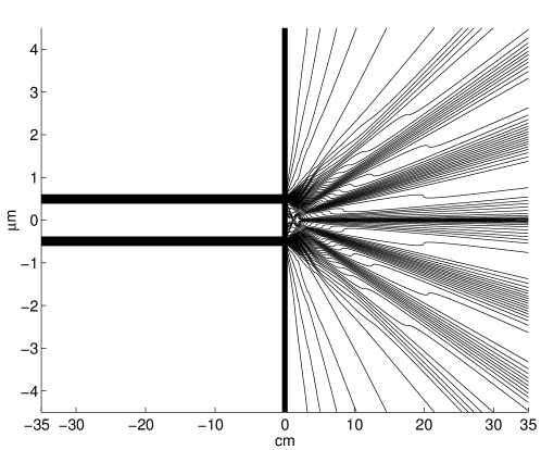
Figure 1: 100 Broglie-Bohm’s trajectories through one of two slits.

Figure 2 shows the 100 previous trajectories when the Planck constant is divided by 10, 100, 1000 and 10000 respectively. We obtain, when h tends to 0, the convergence of quantum trajectories to classic trajectories.

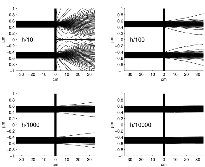
Figure 2: Zoom of the 100 previous trajectories when the Planck constant is divided by 10, 100, 1000 and 10000 respectively.

III Convergence in the determinist semi-classical case

The convergence study of the determinist semi-classical case is mathematically very difficult. We only study the example of a coherent state where an explicit calculation is possible. This example will enable to understand the convergence in the determinist semi-classical case and the difference with the statistical semi-classical case.

For the two dimensional harmonic oscillator, $V(\textbf{x})=\frac{1}{2}m\omega^{2}\textbf{x}^{2}$, coherent states are built CohenTannoudji_1977 from the initial wave function $\Psi_{0}(\textbf{x})$ which corresponds to the density and initial action :

$$\rho^{\hbar}_{0}(\mathbf{x})=(2\pi\sigma_{\hbar}^{2})^{-1}e^{-\frac{(\textbf{x}-\textbf{x}_{0})^{2}}{2\sigma_{\hbar}^{2}}}\qquad and\qquad S_{0}(\mathbf{x})=S^{\hbar}_{0}(\mathbf{x})=m\textbf{v}_{0}\cdot\textbf{x}$$ (12)

with $\sigma_{\hbar}=\sqrt{\frac{\hbar}{2m\omega}}$. Here, $\textbf{v}_{0}$ and $\textbf{x}_{0}$ are still constant vectors and independant from $\hbar$, but $\sigma_{\hbar}$ will tend to $0$ as $\hbar$.

For this harmonic oscillator, the density $\rho^{\hbar}(\textbf{x},t)$ and the action $S^{\hbar}(\textbf{x},t)$,solutions to the Madelung equations (3)(4)(5) with initial conditions (12), are equal to  CohenTannoudji_1977 :

$$\rho^{\hbar}(\textbf{x},t)=\left(2\pi\sigma_{\hbar}^{2}\right)^{-1}e^{-\frac{(\textbf{x}-\xi(t))^{2}}{2\sigma_{\hbar}^{2}}}~{}~{}~{}~{}and~{}~{}~{}~{}S^{\hbar}(\textbf{x},t)=+m\frac{d\xi(t)}{dt}\cdot\textbf{x}+g(t)-\hbar\omega t$$ (13)

where $\xi(t)$ is the trajectory of a classical particle evolving in the potential $V(\textbf{x})=\frac{1}{2}m\omega^{2}\textbf{x}^{2}$, with $\textbf{x}_{0}$ and $\textbf{v}_{0}$ as initial position and velocity and $g(t)=\int_{0}^{t}(-\frac{1}{2}m(\frac{d\xi(s)}{ds})^{2}+\frac{1}{2}m\omega^{2}\xi(s)^{2})ds$. Because we have $2V(\xi(s))=m\frac{d^{2}\xi(s)}{ds^{2}}\cdot\xi(s)$, it yields the following theorem:

THEOREM 3

- When $\hbar\to 0$, the density $\rho^{\hbar}(\textbf{x},t)$ and the action $S^{\hbar}(\textbf{x},t)$ converge to

$$\rho(\textbf{x},t)=\delta(\textbf{x}-\xi(t))~{}~{}and~{}~{}S(\textbf{x},t)=m\frac{d\xi(t)}{dt}\cdot\textbf{x}+g(t)$$ (14)

where $S(\textbf{x},t)$ and the trajectory $\xi(t)$ are solutions to the determinist Hamilton-Jacobi equations:

$$\frac{\partial S\left(\textbf{x},t\right)}{\partial t}|_{\textbf{x}=\xi(t)}+\frac{1}{2m}(\nabla S(\textbf{x},t))^{2}|_{\textbf{x}=\xi(t)}+V(\textbf{x})|_{\textbf{x}=\xi(t)}=0\text{ \ \ \ \ \ \ \ }\forall t\in\mathbb{R}^{+}$$ (15)

$$\frac{d\xi(t)}{dt}=\frac{\nabla S(\xi(t),t)}{m}\text{ \ \ \ \ \ \ \ }\forall t\in\mathbb{R}^{+}$$ (16)

$$S(\textbf{x},0)=m\textbf{v}_{0}\cdot\textbf{x}~{}~{}~{}and~{}~{}~{}\xi(0)=\textbf{x}_{0}.$$ (17)

Therefore, the kinematic of the wave packet converges to the single harmonic oscillator one described by $\xi(t)$. Because this classical particle is completely defined by its initial conditions $\textbf{x}_{0}$ and $\textbf{v}_{0}$, it can be considered as a discerned particle.

When $\hbar\to 0$, the "quantum potential" $Q^{\hbar}(\textbf{x},t)=-\frac{\hbar^{2}}{2m}\frac{\triangle\sqrt{\rho}}{\sqrt{\rho}}=\hbar\omega-\frac{1}{2}m\omega^{2}(\textbf{x}-\xi(t))^{2}$ tends to $Q(\textbf{x},t)=-\frac{1}{2}m\omega^{2}(\textbf{x}-\xi(t))^{2}$. It is then zero on the trajectory ($\textbf{x}=\xi(t)$).

It is then possible to consider, unlike the statistical semi-classical case, that the wave function can be viewed as a single quantum particle. The determinist semi-classical case is in agreement with the Copenhagen interpretation of the wave function which contains all the information on the particle.

III.1 Interpretation for the determinist semi-classical case

In the determinist semi-classical case, the Broglie-Bohm interpretation is not relevant mathematically unlike the statistical semi-classical case. Other assumptions are possible. A natural interpretation is the one proposed by Schrödinger  Schrodinger_26 in 1926 for the coherent states of the harmonic oscillator. In Schrödinger interpretation, the quantum particle in the determinist semi-classical case is a spatially extended particle, represented by a wave packet whose center follows the classical trajectory. In this interpretation, the velocity in each point of the wave function is given byBohm_93 ; Holland_93 ; Holland_99 ; GondranMA :

$$\textbf{v}^{\hbar}(\textbf{x},t)=\frac{1}{m}\nabla S^{\hbar}(\textbf{x},t)+\frac{\hbar}{2m}\nabla\ln\rho^{\hbar}(\textbf{x},t)\times\textbf{k},$$ (18)

where k is the unit vector parallel to the particle spin vector. This spin current $\frac{\hbar}{2m}\nabla\rho^{\hbar}(\textbf{x},t)\times\textbf{k}$ corresponds to Gordon’s current when one changes from Dirac’s equation to Pauli’s equation and after that to Schrodinger’s equationHolland_99 . This current is important because it allows to revisit quantum mechanics at small scales, in particular Compton’s wavelength as in the Foldy and Wouthuysen transformation Foldy . Using this velocity, the Heisenberg inequalities correspond to a dispersion relation position and velocity between the different points of the extended particle.

For the coherent states of the harmonic oscillator in two dimensions, the velocity field (18) is equal to:

$$\textbf{v}^{\hbar}(\mathbf{x},t)=\textbf{v}(t)+\Omega\times(\textbf{x}-\xi(t))$$ (19)

with $\Omega=\omega\textbf{k}$. They behave as extended particles which have the same evolution as spinning particles in two dimensions. But this can not be generalized easily in three dimensions. It seems that it is not possible to consider in three dimensions the particle as a solid in motion. This is the main difficulty in the Schrödinger interpretation: does the particle exist within the wave packet? We think that this reality can only be defined at the scale where the Schrödinger equation is the effective equation. Some solutions are nevertheless possible at smaller scales Gondran_2001 ; Gondran_2004 , where the quantum particle is not represented by a point but is a sort of elastic string whose gravity center follows the classical trajectory $\xi(t)$.

III.2 Interpretation for the non semi-classical case

The Broglie-Bohm and Schrödinger interpretations correspond to the semi-classical approximation. But there exist situations where the semi-classical approximation is not valid. It is in particular the case of state transitions for a hydrogen atom. Indeed, since Delmelt’experiment Delmelt_1986 in 1986, the physical reality of individual quantum jumps has been fully validated. The semi-classical approximation, where the interaction with the potential field can be described classically, is not possible anymore and it is necessary to electromagnetic field quantization since the exchanges are done photon by photon.

In this situation, the Schrödinger equation cannot give a deterministic interpretation and the statistical Born interpretation is the only valid one.

These three interpretations are not new, as Einstein points out in one of his last articles (1953), "Elementary reflexion concerning the quantum mechanics foundation" in a homage to Max Born:

"The fact that the Schrödinger equation associated to the Born interpretation does not lead to a description of the "real states" of an individual system, naturally incites one to find a theory that is not subject to this limitation. Up to now, the two attempts have in common that they conserve the Schrödinger equation and abandon the Born interpretation. The first one, which marks de Broglie’s comeback, was continued by Bohm.… The second one, which aimed to get a "real description" of an individual system and which might be based on the Schrödinger equation is very late and is from Schrödinger himself. The general idea is briefly the following : the function $\psi$ represents in itself the reality and it is not necessary to add it to Born’s statistical interpretation.[…] From previous considerations, it results that the only acceptable interpretation of the Schrödinger equation is the statistical interpretation given by Born. Nevertheless, this interpretation doesn’t give the "real description" of an individual system, it just gives statistical statements of entire systems."

What is new is to consider that these interpretations depend on the preparation of the particles.

Thus, it is because de Broglie and Schrödinger keep the Schrödinger equation that Einstein, who considers it as fundamentaly statistical, rejected each of their interpretations.

Einstein thought that it was not possible to obtain an individual deterministic behavior from the Schrödinger equation. It is the same for Heisenberg who developped matrix mechanics and the second quantization from this example.

This doesn’t mean that one has to renounce determinism and realism, but rather that Schrödinger’s statistical wave function does not permit, in that case, to obtain an individual behavior.

IV Conclusion

The study of the convergence of the Madelung equations when $\hbar\to 0$, has encouraged us to introduce the concept of non-discerned and discerned particles in classical mechanics and has given us the three following results:

- In the statistical semi-classical case the quantum particles converge to classical non-discerned ones verifying the statistical Hamilton-Jacobi equations. The wave function is not sufficient to represent the quantum particles. One needs to add it to the initial positions, as for classical particles, in order to describe them completely. Then, the Broglie-Bohm interpretation is relevant.

- In the determinist semi-classical case the quantum particles converge to classical discerned ones verifying the determinist Hamilton-Jacobi equations. The Broglie-Bohm interpretation is not relevant because the wave function is sufficient to represent the particles as in the Copenhagen interpretation. However, one can make a realistic and deterministic assumption such as the Schrödinger interpretation.

- In the case where the semi-classical approximation is not valid anymore, as in the transition states in the hydrogen atom, the two interpretations are wrong as claimed by Heisenberg. Consequently, Born’s statistical interpretation is the only possible interpretation of the Schrödinger equation. This doesn’t mean that it is necessary to abandon determinism and realism, but rather that the Schrödinger wave function doesn’t allow, in that case, to obtain an individual behavior of a particle. An individual interpretation needs to use creation and annihilation operators of the quantum Field Theory.

Therefore, as Einstein said, the situation is much more complex than de Broglie and Bohm thought.

Each founding father of quantum mechanics held a piece of the truth; but the overgeneralization of their different truths has led to incompatible interpretations!

References

- (1) E. Madelung, "Quantentheorie in hydrodynamischer Form", Zeit. Phys. 40 (1926) 322-6.
- (2) E. Schrödinger, Der stetige bergang von der Mikro-zur Makromechanik, Naturwissenschaften 14 (1926) 664-666.
- (3) R. J. Glauber, dans Quantum Optics and Electronics, Les Houches Lectures 1964, C. deWitt, A. Blandin and C. Cohen-Tanoudji eds., Gordon and Breach, New York, 1965.
- (4) I. Bialynicki-Birula, M. Kalinski, and J. H. Eberly, Phys. Rev. Lett. 73, 1777 (1994).
- (5) A. Buchleitner and D. Delande, Phys. Rev. Lett. 75, 1487 (1995).
- (6) A. Buchleitner, D. Delande and J. Zakrzewski, "Non-dispersive wave packets in periodically driven quantum systems," Physics Reports 368 409-547 (2002).
- (7) H. Maeda and T. F. Gallagher, Non dispersing Wave Packets, Phys. Rev. Lett. 92 (2004) 133004-1.
- (8) R. Feynman and A. Hibbs, Quantum Mechanics and Integrals (McGraw-Hill, 1965).
- (9) M. Gondran, "Analyse MinPlus" C. R. Acad. Sci. Paris 323, 371-375 (1996).
- (10) M. Gondran et M. Minoux, Graphs, Dioïds and Semi-rings: New models and Algorithms, Springer, Operations Research/Computer Science Interfaces (2008).
- (11) V.P. Maslov and S.N. Samborski,Idempotent Analysis , Advancesin Soviet Mathematics, 13, American Math Society, Providence (1992).
- (12) A. Landé, New Foundations of Quantum Mechanics, p. 68 (Cambridge, 1965).
- (13) J. M. Leinaas and J. Myrheim, "On the Theory of Identical Particles", Il Nuovo Cimento, 37 B, 1-23 (1977).
- (14) W. Greiner, L. Neise et H. Stöcker, Thermodynamique et mécanique statistique, Springer, 1999.
- (15) L. de Broglie, J. de Phys. 8, 225-241 (1927).
- (16) D. Bohm, "A suggested interpretation of the quantum theory in terms of ”hidden” variables," Phys. Rev., 85, 166-193 (1952).
- (17) C. Jönsson, “Elektroneninterferenzen an mehreren künstlich hergestellten Feinspalten,” Z. Phy. 161, 454-474 (1961), English translation “Electron diffraction at multiple slits,” Am. J. Phys. 42, 4–11 (1974).
- (18) C. Cohen-Tannoudji, B.Diu, and F. Laloë, Quantum Mechanics, ( Wiley, New York, 1977).
- (19) M. Gondran, and A. Gondran, "Numerical simulation of the double-slit interference with ultracold atoms", Am. J. Phys. 73, 507-515 (2005).
- (20) D. Bohm, B.J. Hiley, The Undivided Universe (Routledge, London and New York, 1993.
- (21) P.R. Holland , The quantum Theory of Motion, (Cambridge University Press, 1993).
- (22) P. R. Holland, "Uniqueness of paths in quantum mechanics," Phys. Rev. A 60, 6 (1999).
- (23) M. Gondran, A. Gondran, "Revisiting the Schrödinger Probability current", quant-ph/0304055 v1.
- (24) L.L. Foldy and S. A. Wouthuysen, Phys. Rev. 78, 29 (1958).
- (25) M. Gondran, "Processus complexe stochastique non standard en mécanique," C. R. Acad. Sci. Paris 333, 592-598 (2001).
- (26) M. Gondran, "Schrödinger Equation and Minplus Complex Analysis", Russian Journal of Mathematical Physics, vol. 11, n2, pp. 130-139 ( 2004).
- (27) W. Nagournay, J. Sandberg, and H. Dehmelt, "Shelved optical electron amplifier: Observation of quantum jumps," Phys. Rev. Lett. 56, 2797-2799 (1986).