An Hi column density threshold for cold gas formation in the Galaxy

Abstract

We report the discovery of a threshold in the Hi column density of Galactic gas clouds below which the formation of the cold phase of Hi is inhibited. This threshold is at ${\rm N_{\sc HI}}=2\times 10^{20}$ per cm²; sightlines with lower Hi column densities have high spin temperatures (median ${\rm T}_{s}\sim 1800$ K), indicating low fractions of the cold neutral medium (CNM), while sightlines with ${\rm N_{\sc HI}}\geq 2\times 10^{20}$ per cm² have low spin temperatures (median ${\rm T}_{s}\sim 240$ K), implying high CNM fractions. The threshold for CNM formation is likely to arise due to inefficient self-shielding against ultraviolet photons at lower Hi column densities. The threshold is similar to the defining column density of a damped Lyman-$\alpha$ absorber; this indicates a physical difference between damped and sub-damped Lyman-$\alpha$ systems, with the latter class of absorbers containing predominantly warm gas.

1. Introduction

The diffuse interstellar medium (ISM) contains gas over a wide range of densities, temperatures and ionization states. These can be broadly sub-divided into the molecular phase (e.g. Snow & McCall 2006), the neutral atomic phase (e.g. Kulkarni & Heiles 1988), and the warm and hot ionized phases (e.g. Haffner et al. 2009). The neutral atomic medium (mostly neutral hydrogen, Hi) is further usually sub-divided into “cold” and “warm” phases (the “CNM” and “WNM”, respectively). Typical CNM temperatures and densities are $\sim 40-200$ K and $\gtrsim 10$ cm^-3, respectively, with corresponding WNM values of $\gtrsim 5000$ K and $\sim 0.1-1$ cm^-3. This was originally an observational definition, to distinguish between phases producing strong narrow absorption lines towards background radio-loud quasars and smooth broad emission lines (Clark 1965). Later, this separation into cold and warm phases was found to arise naturally in the context of models in which the atomic and ionized phases are in pressure equilibrium. Atomic gas at intermediate temperatures was found to be unstable to perturbations, and to migrate to either the cold or warm stable phases, given sufficient time to attain pressure equilibrium (Field et al. 1969; Wolfire et al. 1995).

Radio studies of the Hi-21cm transition have played a vital role in understanding physical conditions in the neutral ISM. The Hi-21cm excitation temperature of a gas cloud (the “spin temperature”, ${\rm T}_{s}$) can be shown to depend on the local kinetic temperature (${\rm T}_{k}$; Field 1959; Liszt 2001), with ${\rm T}_{s}\approx{\rm T}_{k}$ in the CNM and ${\rm T}_{s}\leq{\rm T}_{k}$ in the WNM (Liszt 2001). Since the Hi-21cm absorption opacity for a fixed Hi column density varies inversely with ${\rm T}_{s}$, while the emissivity is independent of ${\rm T}_{s}$ (in the low opacity limit), Hi-21cm absorption studies against background radio sources are primarily sensitive to the presence of CNM along the sightline, while Hi-21cm emission studies are sensitive to both warm and cold Hi. Indeed, the original evidence for two temperature phases in the neutral gas stemmed from a comparison between Hi-21cm absorption and emission spectra (Clark 1965).

Physical conditions in the neutral gas are also known to depend on the gas column density. At the low Hi column densities of the inter-galactic medium, ${\rm N_{\sc HI}}<10^{17}$ cm^-2, the gas is optically thin to ionizing ultraviolet (UV) photons and is hence mostly ionized, giving rise to the so-called Lyman-$\alpha$ forest (Rauch 1998). At higher Hi column densities, $10^{17}\lesssim{\rm N_{\sc HI}}\lesssim 10^{20}$ cm^-2, the Hi is optically-thick to ionizing photons at the Lyman-limit, and the core of the Lyman-$\alpha$ absorption line is saturated. Such “Lyman-limit systems” are partially ionized and typically arise for sightlines through the outskirts of galaxies (Bergeron & Boissé 1991). At still higher Hi column densities, ${\rm N_{\sc HI}}\geq 2\times 10^{20}$ cm^-2, the Lyman-$\alpha$ line becomes optically-thick in its naturally-broadened wings and acquires a Lorentzian shape; such systems are called damped Lyman-$\alpha$ absorbers (DLAs; Wolfe et al. 2005). Damped absorption is ubiquitous on sightlines through galaxy disks and, at high redshifts, has long been used as the signature of the presence of an intervening galaxy along a quasar sightline (Wolfe et al. 1986). Finally, the molecular hydrogen fraction shows a steep transition from very low values to greater than 5% at ${\rm N_{\sc HI}}\sim 5\times 10^{20}$ cm^-2 in the Galaxy (Savage et al. 1977; Gillmon et al. 2006)). Neutral gas is likely to become predominantly molecular at higher Hi column densities, ${\rm N_{\sc HI}}\gtrsim 10^{22}$ cm^-2 (Schaye 2001; Krumholz et al. 2009).

While it is well known that a threshold column density (${\rm N_{\sc HI}}\sim 5\times 10^{20}$ cm^-2) is required to form the molecular phase, for self-shielding against UV photons in the ${\rm H}_{2}$ Lyman band (Stecher & Williams 1967; Hollenbach et al. 1971; Federman et al. 1979), the conditions for CNM formation are less clear. In this Letter, we report results from Hi-21cm absorption studies of a large sample of compact radio sources that indicate the presence of a similar, albeit lower, Hi column density threshold for CNM formation in the Milky Way.

2. The sample

We have used the Westerbork Synthesis Radio Telescope (WSRT, 23 sources), the Giant Metrewave Radio Telescope (GMRT, 10 sources) and the Australia Telescope Compact Array (ATCA, 2 sources) to carry out sensitive, high spectral resolution ($\sim 0.26-0.52$ km/s) Hi-21cm absorption spectroscopy towards 35 compact radio-loud quasars. Most of the target sources were selected to be B-array calibrators for the Very Large Array, and have angular sizes $\lesssim 5^{\prime\prime}$. Details of the sample selection, observations and data analysis are given in Kanekar et al. (2003), Braun & Kanekar (2005), Roy et al. (2011, in prep.) and Kanekar & Braun (2011, in prep.). The final optical-depth spectra have root-mean-square (RMS) noise values of $\tau_{\rm RMS}\sim 0.0002-0.0013$ per 1 km/s channel, with a median RMS noise of $\sim 5\times 10^{-4}$ per 1 km/s channel. These RMS noise values are at off-line channels, away from Hi-21cm emission that increases the system temperature, and hence, the RMS noise. A careful bandpass calibration procedure was used to ensure a high spectral dynamic range and excellent sensitivity to wide absorption [see Kanekar et al. (2003) and Braun & Kanekar (2005) for details]. These are among the deepest Hi-21cm absorption spectra ever obtained (e.g. Dwarakanath et al. 2002; Kanekar et al. 2003; Begum et al. 2010) and constitute by far the largest sample of absorption spectra of this sensitivity. The use of interferometry also implies that the spectra are not contaminated by Hi-21cm emission within the beam, unlike the case with single-dish absorption spectra (Kanekar et al. 2003; Heiles & Troland 2003).

Galactic Hi-21cm absorption was detected against every source but one, B0438-436. We used the Leiden-Argentine-Bonn (LAB) survey (Kalberla et al. 2005) to estimate the “apparent” Hi column density (uncorrected for self-absorption, i.e. ${\rm N_{\sc HI}}=1.823\times 10^{18}\times\int T_{B}{\rm dV}$ cm^-2 (Wilson et al. 2009), where $T_{B}$ is the brightness temperature) at a location adjacent to each target. The observational results are summarized in Table 1, whose columns contain (1) the quasar name, (2) its Galactic latitude, (3) the Hi column density (uncorrected for self-absorption), in units of $10^{20}$ cm^-2, from the LAB survey, (4) the integrated Hi-21cm optical depth $\int\tau{\rm dV}$, in km/s, and (5) the harmonic-mean spin temperature ${\rm T}_{s}$ in K, estimated assuming the low optical depth limit (${\rm T}_{s}=\int T_{B}{\rm dV}/\int\tau{\rm dV}$).

Finally, for the one source with undetected Hi-21cm absorption (B0438-436), we quote a $3\sigma$ upper limit on the integrated Hi-21cm optical depth, assuming a Gaussian line profile with a full width at half maximum of 20 km/s, and the corresponding $3\sigma$ lower limit on the spin temperature.

Table 1The full sample of 35 sources.

QSO	Latitude	N${}_{\rm HI}\>^{a}$	$\int\tau\rm{dV}\>^{b}$	${\rm T}_{s}$
	$b$	$\times 10^{20}$ cm-2	km s-1	K
B0023-263	-84.17	$1.641\pm 0.022$	$0.025\pm 0.005$	$3546\pm 694$
B0114-211	-81.47	$1.380\pm 0.034$	$0.135\pm 0.005$	$559\pm 26$
B0117-156	-76.42	$1.418\pm 0.034$	$0.031\pm 0.004$	$2538\pm 353$
B0134+329	-28.72	$4.272\pm 0.029$	$0.443\pm 0.002$	$530\pm 4$
B0202+149	-44.04	$4.809\pm 0.027$	$0.747\pm 0.005$	$353\pm 3$
B0237-233	-65.13	$2.078\pm 0.038$	$0.294\pm 0.004$	$388\pm 9$
B0316+162	-33.60	$9.431\pm 0.034$	$2.964\pm 0.004$	$175\pm 1$
B0316+413	-13.26	$13.234\pm 0.028$	$1.941\pm 0.003$	$374\pm 1$
B0355+508	-1.60	$74.344\pm 0.079$	$45.820\pm 1.120$	$89\pm 2$
B0404+768	18.33	$10.879\pm 0.032$	$1.945\pm 0.005$	$307\pm 1$
B0407-658	-40.88	$3.363\pm 0.018$	$0.548\pm 0.007$	$337\pm 5$
B0429+415	-4.34	$37.067\pm 0.041$	$10.879\pm 0.007$	$187\pm 1$
B0438-436	-41.56	$1.380\pm 0.027$	$<0.020$	$>3785$
B0518+165	-11.34	$20.616\pm 0.035$	$6.241\pm 0.007$	$181\pm 1$
B0531+194	-7.11	$26.609\pm 0.036$	$4.062\pm 0.005$	$359\pm 1$
B0538+498	10.30	$19.542\pm 0.029$	$5.618\pm 0.003$	$191\pm 1$
B0831+557	36.56	$4.469\pm 0.032$	$0.483\pm 0.006$	$507\pm 7$
B0834-196	12.57	$7.125\pm 0.036$	$0.973\pm 0.005$	$402\pm 3$
B0906+430	42.84	$1.251\pm 0.036$	$0.051\pm 0.003$	$1342\pm 89$
B1151-348	26.34	$7.732\pm 0.031$	$0.714\pm 0.005$	$594\pm 5$
B1245-197	42.88	$3.802\pm 0.037$	$0.158\pm 0.005$	$1323\pm 40$
B1323+321	81.05	$1.260\pm 0.034$	$0.083\pm 0.003$	$836\pm 40$
B1328+254	80.99	$1.065\pm 0.036$	$0.021\pm 0.003$	$2729\pm 411$
B1328+307	80.67	$1.197\pm 0.030$	$0.072\pm 0.002$	$916\pm 32$
B1345+125	70.17	$1.957\pm 0.024$	$0.305\pm 0.005$	$352\pm 7$
B1611+343	46.38	$1.318\pm 0.034$	$0.019\pm 0.003$	$3873\pm 565$
B1641+399	40.95	$1.044\pm 0.032$	$0.009\pm 0.002$	$6498\pm 1760$
B1814-637	-20.76	$6.416\pm 0.018$	$0.997\pm 0.007$	$353\pm 3$
B1827-360	-29.34	$8.163\pm 0.018$	$1.542\pm 0.003$	$290\pm 1$
B1921-293	-11.78	$7.312\pm 0.017$	$1.446\pm 0.006$	$277\pm 1$
B2050+364	-48.84	$27.638\pm 0.038$	$3.024\pm 0.010$	$501\pm 2$
B2200+420	-5.12	$17.119\pm 0.042$	$3.567\pm 0.016$	$263\pm 1$
B2203-188	-51.16	$2.432\pm 0.018$	$0.248\pm 0.004$	$537\pm 10$
B2223-052	-10.44	$4.561\pm 0.030$	$1.034\pm 0.003$	$242\pm 2$
B2348+643	2.56	$70.522\pm 0.051$	$32.517\pm 0.031$	$119\pm 1$

Notes: ^a From the LAB emission survey. ^b From our Hi-21cm absorption survey.

3. Results: An ${\rm N_{\sc HI}}$ threshold for CNM formation

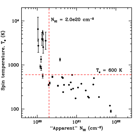
Figure 1.— [A] Left panel: The integrated optical depth $\int\tau{\rm dV}$ (in km/s), from our Hi-21cm absorption survey, plotted against apparent Hi column density (cm^-2), from the LAB emission survey; the dashed curves show the relation in eqn. 3 with $(log(N_{0}),log(N_{\infty}),\Delta V)$ = (20.0, 21.7, 20) and (20.3, 22.0, 10). [B] Right panel: The column-density-weighted harmonic mean spin temperature (K) plotted against apparent Hi column density (cm^-2).

The left panel of Figure 1 shows the integrated Hi-21cm optical depth plotted against Hi column density, on a logarithmic scale. It is clear from the figure that the integrated Hi-21cm optical depth has a rough power-law dependence on ${\rm N_{\sc HI}}$ for ${\rm N_{\sc HI}}\geq 2\times 10^{20}$ cm^-2. However, there is a steep decline in $\int\tau{\rm dV}$ for Hi column densities lower than this value. These properties were noted previously by Braun & Walterbos (1992) for individual spectral features (see their Figs. 3–6) rather than the line-of-sight integral. A similar pattern is visible in the right panel of the figure, which plots the spin temperature ${\rm T}_{s}$ against ${\rm N_{\sc HI}}$. 24 out of 25 sightlines with ${\rm N_{\sc HI}}\geq 2\times 10^{20}$ cm^-2 show ${\rm T}_{s}<600$ K, while all ten sightlines with ${\rm N_{\sc HI}}<2\times 10^{20}$ cm^-2 have ${\rm T}_{s}>550$ K. The median spin temperature for sightlines with ${\rm N_{\sc HI}}\geq 2\times 10^{20}$ cm^-2 is $\sim 240$ K, while that for sightlines with ${\rm N_{\sc HI}}<2\times 10^{20}$ K is $\sim 1800$ K. Thus, there appears to be a physical difference between sightlines with Hi columns lower and higher than the column density ${\rm N_{LIM}}=2\times 10^{20}$ cm^-2. Note that the use of apparent ${\rm N_{\sc HI}}$ only affects high-opacity sightlines, and has no significant effect on our results.

We used a number of non-parametric two-sample tests (e.g. the Gehan test, the Peto-Prentice test, the logrank test, etc), generalized for censored data, to determine whether the spin temperatures of sightlines with ${\rm N_{\sc HI}}\geq{\rm N_{\sc LIM}}$ and ${\rm N_{\sc HI}}<{\rm N_{\sc LIM}}$ are drawn from the same parent distribution. All tests used the ASURV Rev. 1.2 package (Lavalley et al. 1992) which implements the methods of Feigelson & Nelson (1985). The use of multiple tests guards against any biases within a given test, resulting from the relatively small sample size (10 systems with ${\rm N_{\sc HI}}<{\rm N_{\sc LIM}}$) and the presence of censored values (Feigelson & Nelson 1985). Errors on individual measurements were handled through a Monte-Carlo approach, using the measured values of ${\rm T}_{s}$ and ${\rm N_{\sc HI}}$ (and the associated errors) for each sightline to generate $10^{4}$ sets of 35 pairs of ${\rm T}_{s}$ and ${\rm N_{\sc HI}}$ values. The statistical significance of each result (quoted below) is the average of values obtained in these $10^{4}$ trials for each test. The tests found clear evidence, with statistical significance between $4.2\sigma$ and $5.3\sigma$ that the spin temperatures for sightlines with ${\rm N_{\sc HI}}\geq{\rm N_{\sc LIM}}$ and ${\rm N_{\sc HI}}<{\rm N_{\sc LIM}}$ are drawn from different parent populations. Following Feigelson & Nelson (1985), our final result is based on the Peto-Prentice test, as this has been found to give the best results for very different sample sizes (Latta 1981). The two ${\rm T}_{s}$ sub-samples (with “low” and “high” ${\rm N_{\sc HI}}$) are then found to be drawn from different parent distributions at $5.3\sigma$ significance; the probability of this arising by chance is $\sim 2\times 10^{-7}$.

It thus appears that sightlines with ${\rm N_{\sc HI}}<{\rm N_{\sc LIM}}=2\times 10^{20}$ cm^-2 have systematically higher spin temperatures than sightlines with ${\rm N_{\sc HI}}>{\rm N_{\sc LIM}}$. The spin temperature measured here is the column-density-weighted harmonic mean of the spin temperatures of different “phases” along the line of sight (e.g. Kulkarni & Heiles 1988). For example, a sightline with ${\rm N_{\sc HI}}$ equally divided between CNM and WNM, with ${\rm T}_{s}=100$ K and ${\rm T}_{s}=8000$ K respectively, would yield an average ${\rm T}_{s}\sim 200$ K, while one with 90% of gas with ${\rm T}_{s}=8000$ K and 10% with ${\rm T}_{s}=100$ K would yield an average ${\rm T}_{s}=900$ K. In other words, a high ${\rm T}_{s}$ indicates the presence of a smaller fraction of the cold phase of Hi. Thus, the fact that average spin temperatures are significantly higher on sightlines with low Hi column densities, ${\rm N_{\sc HI}}<2\times 10^{20}$ cm^-2, indicates that such low-${\rm N_{\sc HI}}$ sightlines contain low CNM fractions, far smaller than those on sightlines with ${\rm N_{\sc HI}}\geq 2\times 10^{20}$ cm^-2.

It is clear from Fig. 1[A] that the integrated Hi-21cm optical depth drops sharply at ${\rm N_{\sc HI}}={\rm N_{\sc LIM}}$, due to the decline in the CNM fraction at low Hi column densities. This can be accounted for by a simple physical model in which a minimum “shielding” Hi column density of WNM is needed for the formation of the cold phase in an Hi cloud. Assuming that the Hi-21cm optical depth in the WNM is negligible compared to that in the CNM, the equation of radiative transfer for a “sandwich” geometry can be written as

$$T_{B}{\rm(V)}=\frac{T_{w}\tau_{w}}{2}+T_{c}(1-e^{-\tau_{c}})+\frac{T_{w}\tau_{w}}{2}e^{-\tau_{c}}$$ (1)

where the explicit velocity dependence of $\tau_{W}$ and $\tau_{C}$ has been omitted for clarity and the integrated Hi emission profile becomes,

$$\int T_{B}{\rm dV}=\int T_{w}\tau_{w}e^{-\tau_{c}}{\rm dV}+\int\bigg{(}T_{c}+\frac{T_{w}\tau_{w}}{2}\bigg{)}(1-e^{-\tau_{c}}){\rm dV}$$ (2)

or,

$$N^{\prime}_{HI}=N_{0}e^{-\tau_{c}^{\prime}}+N_{\infty}(1-e^{-\tau_{c}^{\prime}})$$ (3)

for a measured “apparent” column density, $N^{\prime}_{\rm HI}$ (assuming negligible self-opacity), a threshold column density (where $\tau_{c}\rightarrow 0$), $N_{0}\sim T_{w}\tau_{w}\Delta V$, a saturation column density (where $\tau_{c}\rightarrow\infty$), $N_{\infty}\sim(T_{c}+T_{w}\tau_{w}/2)\Delta V$ and an effective opacity, $\tau_{c}^{\prime}$. The effective opacity is related to the measured integrated opacity by the effective linewidth, $\Delta V$, as $\int\tau{\rm dV}=\tau_{c}^{\prime}\Delta V$.

The upper and lower dashed curves in Fig. 1[A] show the above expression for (${\rm N_{0}}=10^{20}$ cm^-2, ${\rm N_{\infty}}=5.0\times 10^{21}$ cm^-2, $\Delta V=20$ km/s) and (${\rm N_{0}}=2\times 10^{20}$ cm^-2, ${\rm N_{\infty}}=10^{22}$ cm^-2, $\Delta V=10$ km/s), respectively. Note that the effective linewidth only shifts the curves up and down in the figure. The fact that none of the data points of Fig. 1[A] lie to the left of the upper curve indicates that a minimum shielding Hi column of $[N_{0}/2]\sim 5\times 10^{19}$ cm^-2 is needed for the formation of the cold neutral medium. Note that, in the above “sandwich” geometry, a total WNM column density of $\gtrsim 10^{20}$ cm^-2 is needed before any CNM can be formed.

4. Discussion

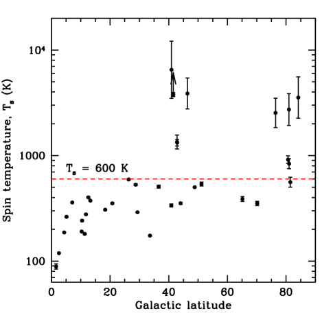
Figure 2.— The column-density-weighted harmonic mean spin temperature (K) plotted against Galactic latitude.

Most theoretical models of the diffuse interstellar medium treat it as a multi-phase medium, consisting of neutral and ionized phases in pressure equilibrium (e.g. Field et al. 1969; McKee & Ostriker 1977; Wolfire et al. 1995). In the McKee-Ostriker model, physical conditions in the ISM are regulated by supernova explosions, whose blast waves sweep up gas in the ISM into shells, leaving large cavities full of hot ionized gas (McKee & Ostriker 1977). Cold atomic gas is then formed by the rapid cooling of the swept-up and shocked gas. Soft X-rays from neighbouring hot ionized gas and stellar UV photons penetrate into the CNM and heat and partially ionize it, producing envelopes of warm neutral and warm ionized gas (WIM). Thus, a typical ISM “cloud” [see Fig. 1 of McKee & Ostriker (1977)] is expected to form at the edges of supernova remnants and super-bubbles containing the hot ionized medium (HIM). Such a cloud consists of a CNM core surrounded by a WNM envelope and a further WIM shell, all of which are in pressure equilibrium. The CNM core is almost entirely neutral, the WNM and WIM are partially ionized, and the HIM is almost entirely ionized (McKee & Ostriker 1977).

A threshold Hi column density for CNM formation in an ISM cloud arises quite naturally due to the need for self-shielding against ionizing ultraviolet (and soft X-ray) photons (see also Schaye 2004). At low Hi columns, UV photons can penetrate all the way into a cloud core and heat (and partly ionize) the Hi. Only clouds that self-shield against the penetration of these high-energy photons can retain a stable CNM core. Self-shielding against UV photons is significant once the optical depth at the Lyman limit crosses unity, i.e. for ${\rm N_{\sc HI}}\geq 10^{17}$ cm^-2, and becomes more and more efficient with increasing Hi column density. Our results indicate that self-shielding only becomes entirely efficient at excluding UV photons from the interior of Hi clouds at a total Hi column density of ${\rm N_{\sc HI}}\sim 2\times 10^{20}$ cm^-2. Below this threshold, sufficient UV photons penetrate into the cloud interior to hinder the survival of the cold phase. The simple “sandwich” model overlaid on Fig. 1[A] suggests that a shielding column of $\sim(0.5-0.75)\times 10^{20}$ cm^-2 on each exposed surface of a cloud is sufficient to exclude UV photons, with the rest of the Hi then free to cool to lower temperatures.

It is also possible that sightlines with low ${\rm N_{\sc HI}}$ are sampling gas at higher distances from the Galactic plane, with lower metallicity and pressure. Two-phase models that incorporate detailed balancing of heating and cooling rates obtain lower CNM fractions at lower pressures and metallicities (Wolfire et al. 1995). Observationally, Kanekar et al. (2009) have found evidence for an anti-correlation between spin temperature and metallicity in high-$z$ DLAs, with low-metallicity DLAs having higher spin temperatures, probably because the paucity of metals yields fewer cooling routes (Kanekar & Chengalur 2001). If low-${\rm N_{\sc HI}}$ sightlines contain “clouds” with systematically lower metallicities (and/or pressures), these could have lower cooling rates and hence, lower CNM fractions. Unfortunately, we do not have estimates of either pressure or metallicity along our sightlines and hence cannot test this possibility. We note that all sightlines with high spin temperatures are at intermediate or high Galactic latitudes, $b>40^{\circ}$ (see Fig. 2), suggesting larger distances from the plane. Conversely, the figure also shows that low spin temperatures ($\lesssim 400$ K) are obtained even for sightlines at high Galactic latitudes ($b\sim 40-70^{\circ}$). Measurements of the metallicity and pressure along the low-${\rm N_{\sc HI}}$ sightlines, through UV spectroscopy, would be of much interest.

There have been earlier suggestions, based on semi-analytical or numerical treatments of self-shielding, that Hi clouds are predominantly neutral for ${\rm N_{\sc HI}}\gtrsim 10^{20}$ cm^-2 (e.g. Viegas 1995; Wolfe et al. 2005). However, this is the first direct evidence for a change in physical conditions in Hi clouds at this column density. Note that this is a factor of several lower than the known threshold of ${\rm N_{\sc HI}}\sim 5\times 10^{20}$ cm^-2 for the formation of molecular hydrogen in Galactic clouds, set by the requirement of self-shielding against UV photons at wavelengths in the H₂ Lyman band (Savage et al. 1977). Thus, there appear to be three column densities at which phase transitions occur in ISM clouds, at ${\rm N_{\sc HI}}\sim 2\times 10^{20}$ cm^-2 resulting in the formation of cold Hi, at ${\rm N_{\sc HI}}\sim 5\times 10^{20}$ cm^-2 resulting in the formation of molecular hydrogen, and finally, at ${\rm N_{\sc HI}}>10^{22}$ cm^-2, when most of the atomic gas is converted into the molecular phase.

In this context, it is vital to appreciate that the abscissa of Fig. 1 refers to apparent  Hi column density under the assumption of negligible self-opacity of the Hi profile. The saturation column density, N_∞, is an observational upper limit to $\int T_{B}dV$ and does not represent a physical limit on ${\rm N_{\sc HI}}$. In fact, the widespread occurrence of the Hi self-absorption phenomenon within the Galaxy (Gibson et al. 2005) and the detailed modeling of high resolution extragalactic Hi spectra suggests that self-opacity is a common occurrence (Braun et al. 2009) which can disguise neutral column densities that reach ${\rm N_{\sc HI}}\sim 10^{23}$ cm^-2.

The original definition of a DLA as an absorber with ${\rm N_{\sc HI}}\geq 2\times 10^{20}$ cm^-2 was an observational one, based on the requirement that the damping wings of the Lyman-$\alpha$ line be detectable in low-resolution optical spectra of moderate sensitivity (Wolfe et al. 1986). With today’s 10-m class optical telescopes, it is easy to detect the damping wings at significantly lower Hi column densities, $\sim 10^{19}$ cm^-2(e.g. Péroux et al. 2003); such systems are referred to as “sub-DLAs”. There has been much debate in the literature on whether or not DLAs and sub-DLAs should be treated as a single class of absorber and on their relative importance in contributing to the cosmic budget of neutral hydrogen and metals (e.g. Péroux et al. 2003; Wolfe et al. 2005; Kulkarni et al. 2010). Wolfe et al. (2005) argue that DLAs and sub-DLAs are physically different, claiming that most of the Hi in sub-DLAs is ionized and at high temperature, while that in DLAs is mostly neutral; this is based on numerical estimates of self-shielding in DLAs and sub-DLAs against the high-$z$ UV background (Viegas 1995). Our detection of an Hi column density threshold for CNM formation that matches the defining DLA column density indicates that DLAs and sub-DLAs are indeed physically different types of absorbers, with sub-DLAs likely to have significantly lower CNM fractions than DLAs, at a given metallicity.

In summary, we report the discovery of a threshold Hi column density, ${\rm N_{\sc HI}}\sim 2\times 10^{20}$ cm^-2, for cold gas formation in Hi clouds in the interstellar medium. Above this threshold, the majority of Galactic sightlines have low spin temperatures, ${\rm T}_{s}\lesssim 500$ K, with a median value of $\sim 240$ K. Below this threshold, typical sightlines have far higher spin temperatures, $>600$ K, with a median value of $\sim 1800$ K. The threshold for CNM formation appears to arise naturally due to the need for self-shielding against ultraviolet photons, which penetrate into the cloud at lower Hi columns and heat and ionize the Hi, inhibiting the formation of the cold neutral medium.

References

- Begum et al. (2010) Begum, A., Stanimirović, S., Goss, W. M., Heiles, C., Pavkovich, A. S., & Hennebelle, P. 2010, ApJ, 725, 1779
- Bergeron & Boissé (1991) Bergeron, J. & Boissé, P. 1991, A&A, 243, 344
- Braun & Kanekar (2005) Braun, R. & Kanekar, N. 2005, A&A, 436, L53
- Braun et al. (2009) Braun, R., Thilker, D. A., Walterbos, R. A. M., & Corbelli, E. 2009, ApJ, 695, 937
- Braun & Walterbos (1992) Braun, R. & Walterbos, R. 1992, ApJ, 386, 120
- Clark (1965) Clark, B. G. 1965, ApJ, 142, 1398
- Dwarakanath et al. (2002) Dwarakanath, K. S., Carilli, C. L., & Goss, W. M. 2002, ApJ, 567, 940
- Federman et al. (1979) Federman, S. R., Glassgold, A. E., & Kwan, J. 1979, ApJ, 227, 466
- Feigelson & Nelson (1985) Feigelson, E. D. & Nelson, P. I. 1985, ApJ, 293, 192
- Field (1959) Field, G. B. 1959, ApJ, 129, 536
- Field et al. (1969) Field, G. B., Goldsmith, D. W., & Habing, H. J. 1969, ApJ, 155, L149
- Gibson et al. (2005) Gibson, S. J., Taylor, A. R., Higgs, L. A., Brunt, C. M., & Dewdney, P. E. 2005, ApJ, 626, 195
- Gillmon et al. (2006) Gillmon, K., Shull, J. M., Tumlinson, J., & Danforth, C. 2006, ApJ, 636, 891
- Haffner et al. (2009) Haffner, L. M., Dettmar, R., Beckman, J. E., Wood, K., Slavin, J. D., Giammanco, C., Madsen, G. J., Zurita, A., & Reynolds, R. J. 2009, Rev. Mod. Phys., 81, 969
- Heiles & Troland (2003) Heiles, C. & Troland, T. H. 2003, ApJS, 145, 329
- Hollenbach et al. (1971) Hollenbach, D. J., Werner, M. W., & Salpeter, E. E. 1971, ApJ, 163, 165
- Kalberla et al. (2005) Kalberla, P. M. W., Burton, W. B., Hartmann, D., Arnal, E. M., Bajaja, E., Morras, R., & Pöppel, W. G. L. 2005, A&A, 440, 775
- Kanekar & Chengalur (2001) Kanekar, N. & Chengalur, J. N. 2001, A&A, 369, 42
- Kanekar et al. (2009) Kanekar, N., Smette, A., Briggs, F. H., & Chengalur, J. N. 2009, ApJ, 705, L40
- Kanekar et al. (2003) Kanekar, N., Subrahmanyan, R., Chengalur, J. N., & Safouris, V. 2003, MNRAS, 346, L57
- Krumholz et al. (2009) Krumholz, M. R., Ellison, S. L., Prochaska, J. X., & Tumlinson, J. 2009, ApJ, 701, L12
- Kulkarni & Heiles (1988) Kulkarni, S. R. & Heiles, C. 1988, in Galactic and Extra-Galactic Radio Astronomy, ed. G. L. Verschuur & K. I. Kellermann (Springer-Verlag New York), 95
- Kulkarni et al. (2010) Kulkarni, V. P., Khare, P., Som, D., Meiring, J., York, D. G., Péroux, C., & Lauroesch, J. T. 2010, New Astronomy, 15, 735
- Latta (1981) Latta, R. B. 1981, J. Am. Statistical Association, 26, 713
- Lavalley et al. (1992) Lavalley, M. P., Isobe, T., & Feigelson, E. D. 1992, in Bulletin of the American Astronomical Society, Vol. 24, 839
- Liszt (2001) Liszt, H. 2001, A&A, 371, 698
- McKee & Ostriker (1977) McKee, C. F. & Ostriker, J. P. 1977, ApJ, 218, 148
- Péroux et al. (2003) Péroux, C., Dessauges-Zavadsky, M., D’Odorico, S., Kim, T., & McMahon, R. G. 2003, MNRAS, 345, 480
- Rauch (1998) Rauch, M. 1998, ARA&A, 36, 267
- Savage et al. (1977) Savage, B. D., Bohlin, R. C., Drake, J. F., & Budich, W. 1977, ApJ, 216, 291
- Schaye (2001) Schaye, J. 2001, ApJ, 562, L95
- Schaye (2004) —. 2004, ApJ, 609, 667
- Snow & McCall (2006) Snow, T. P. & McCall, B. J. 2006, ARA&A, 44, 367
- Stecher & Williams (1967) Stecher, T. P. & Williams, D. A. 1967, ApJ, 149, L29
- Viegas (1995) Viegas, S. M. 1995, MNRAS, 276, 268
- Wilson et al. (2009) Wilson, T. L., Rohlfs, K., & Hüttemeister, S. 2009, Tools of Radio Astronomy (Springer-Verlag: Berlin)
- Wolfe et al. (2005) Wolfe, A. M., Gawiser, E., & Prochaska, J. X. 2005, ARA&A, 43, 861
- Wolfe et al. (1986) Wolfe, A. M., Turnshek, D. A., Smith, H. E., & Cohen, R. D. 1986, ApJS, 61, 249
- Wolfire et al. (1995) Wolfire, M. G., Hollenbach, D., McKee, C. F., Tielens, A. G. G. M., & Bakes, E. L. O. 1995, ApJ, 443, 152