The $T=0$ RFIM on a Bethe lattice: correlation functions along the hysteresis loop

Abstract

We consider the Gaussian random field Ising model (RFIM) on the Bethe lattice at zero temperature in the presence of a uniform external field and derive the exact expressions of the two-point spin-spin and spin-random field correlation functions along the saturation hysteresis loop. To complete the analytical description and suggest possible approximations for the RFIM on Euclidian lattices we also compute the corresponding direct correlation functions (or proper vertices) and show that they decay rapidly with the distance in the weak-coupling/large disorder regime; their range, however, is not limited to the nearest-neighbor distance.

I Introduction

The random field Ising model (RFIM) at zero temperature is a simple prototype of a class of disordered systems (such as random magnets, martensitic materials, fluids in porous solids,…) that exhibit hysteretic and jerky behavior when slowly driven by an external fieldSDP2006 . The most interesting feature of the model which has been the subject of extensive analytical and numerical studies is the existence of a disorder-induced nonequilibrium phase transition between two different regimes of avalanchesSDKKRS1993 . This transition manifests through a change in the shape of the magnetization hysteresis loop that evolves from continuous to discontinuous as the disorder strength is reduced. The discontinuity is associated to a macroscopic avalanche involving a finite fraction of the spins in the thermodynamic limit. As shown recently, this type of mechanism plausibly explains the hysteretic behavior of ⁴He adsorbed in high porosity silica aerogelsDKRT2005 ; B2008 . Interestingly, this nontrivial behavior is already present on the Bethe lattice (i.e. the infinite Cayley tree) where a fully analytical characterization of the major and minor hysteresis loops, the avalanche size distribution, and other quantities can be obtained thanks to the tree topologyDSS1997 ; CGZ2002 ; ABCDDMZ2005 ; IOV2005 ; OS2010 . In this case, the out-of-equilibrium phase transition occurs when the coordination number $z\geq 4$ and is described by a traditional saddle-node transition in the self-consistent field equationDSS1997 (which makes the critical behavior the same as that for the infinite-range mean-field model). In this work we extend the analytical description to the spin-spin and spin-random field correlation (or Green’s) functions along the hysteresis loop, using the fact that correlations on a tree-like graph have a one-dimensional character. For a Gaussian distribution of the random fields, the spin-random field correlation function is also related to the slope of the magnetization curve through a ‘susceptibility’ sum-rule. The motivation for this calculation is twofold. First, on the theoretical side, Green’s functions (or, better, their matrix inverse, the so-called direct correlation functions in liquid state theory or proper vertices in field-theoretic language) may be used as the building blocks of approximate theories, as illustrated by the recent computation of the hysteresis loop in the three-dimensional soft-spin random field modelRT2010 . Exact results, even for simple models, may give some insight of the actual structure of these functions. Secondly, on the experimental side, scattering methods are now frequently combined with other standard probes (response to an applied field or thermodynamic measurements) for extracting information on the structure and the dynamics of systems with quenched randomness (see e.g. Ref. H2004 in the case of fluids adsorbed in porous solids). Knowing the structure of the correlation functions can thus make easier the interpretation of the scattered intensityDKRT2006 .

The outline of the paper is as follows. In section II, we define the model and give the expressions of the correlation functions, first for the one-dimensional chain (correcting the result obtained in Ref.KFS2000 ), and then generalizing to the Bethe lattice (the detailed calculations are presented in Appendices A and B). Analytical predictions are compared to simulations performed on regular random graphs. In section III, we compute the corresponding direct correlation functions. We then conclude.

II Model and correlation functions

The RFIM is defined by the following Hamiltonian

$${\cal H}=-J\sum_{<ij>}S_{i}S_{j}+\sum_{i}(H+h_{i})S_{i}$$ (1)

where the $N$ spins $S_{i}=\pm 1$ are placed on the vertices of a Bethe lattice with coordination number $z$. The first sum is restricted to nearest-neighbors (n.n.) pairs and $J>0$. $H$ is a uniform external field and the fields $\{h_{i}\}$ are random variables drawn independently from a Gaussian distribution $\rho(h)=\exp(-h^{2}/2\Delta)/\sqrt{2\pi\Delta}$ with the variance $\Delta$ measuring the strength of disorder.

The relaxation dynamics is the $T=0$ limit of the Glauber dynamics and consists in aligning the spins with their local effective field at each time stepSDKKRS1993 ,

$$S_{i}=\mbox{sgn}(f_{i})$$ (2)

where

$$f_{i}=-\frac{\partial{\cal H}}{\partial S_{i}}=J\sum_{j/i}S_{j}+H+h_{i}$$ (3)

and the sum runs over the $z$ nearest neighbors of site $i$. The dynamics thus proceeds via a series of avalanches which stop when a metastable state is reached, i.e., when all spins satisfy Eq. (2). The saturation hysteresis loop is obtained by adiabatically ramping $H$ from $-\infty$ to $+\infty$ and back. Thanks to the tree topology of the Bethe lattice and the abelian property of the dynamics (e.g. the fact that the metastable state after an avalanche does not depend on the order in which the spins flip), the shape of the hysteresis loop can be exactly derived. According to Ref.DSS1997 , the magnetization $m(H)$ along the lower half (ascending) branch is given by

$$\frac{1}{2}[m(H)+1]=\sum_{k=0}^{z}{z\choose k}P^{*}(H)^{k}[1-P^{*}(H)]^{z-k}p_{k}(H)$$ (4)

where $p_{k}(H)$ ($k=0..z$) is the probability for a down spin to flip up at the field $H$ when $k$ of its $z$ nearest neighbors are up,

$$p_{k}(H)=\int_{(z-2k)J-H}^{+\infty}\rho(h)dh=\frac{1}{2}\mbox{erfc}\left(\frac{(z-2k)J-H}{\sqrt{2\Delta}}\right)\ ,$$ (5)

(here $\mbox{erfc}(x)=(2/\sqrt{\pi})\int_{x}^{\infty}du\exp(-u^{2})$ is the complementary error function), and $P^{*}(H)$ is solution of the self-consistent equation

$$P^{*}(H)=\sum_{k=0}^{z-1}{z-1\choose k}P^{*}(H)^{k}[1-P^{*}(H)]^{z-1-k}p_{k}(H)\ .$$ (6)

This key quantity represents the conditional probability that a nearest neighbor of spin $i$ flips up before spin $i$. For $z\geq 4$, the polynomial equation (6) has several solutions at low enough disorder (for $\Delta<\Delta_{c}(z)$) and the magnetization displays a jump discontinuity at a coercive field $H_{c}(\Delta)$.

In the following we are interested in calculating the correlations along the loop between the spin at site $i$ and the spin or the random field at site $j$,

$$G^{ss}_{ij} =\overline{S_{i}}\overline{S_{j}}-\overline{S_{i}}\ \overline{S_{j}}$$

$$G^{sh}_{ij} =\overline{S_{i}h_{j}}$$ (7)

where the overbar denotes the average over the random field distribution $\rho(h)$ and the dependence on the applied field $H$ is implicit (hence $\overline{S_{i}}\equiv m(H)$ as given by Eq.(4) along the ascending branch). Due to the average over disorder, the two functions only depend on the distance between the two spins, i.e. on $n$, the number of bonds between $i$ and $j$. We thus denote them by $G^{ss}(n)$ and $G^{sh}(n)$, respectively.

Let us recall that at finite temperature and equilibrium, because of the additional average over thermal fluctuations, there are two distinct spin-spin correlation functions, $\overline{<S_{i}S_{j}>-<S_{i}><S_{j}>}$ and $\overline{<S_{i}S_{j}>}-\overline{<S_{i}>}\ \overline{<S_{j}>}$ where $<...>$ denotes the thermal averageN1998 . The former (the so-called connected or truncated function) may be non-zero at $T=0$ if the ground state of the system is highly degenerate. This does not occur when the random-field distribution is continuous and then only the disconnected function $G^{ss}(n)$ remains non-zero. At $T=0$, one may also consider an average over all the metastable states at a given field $H$ and then distinguish again connected and disconnected contributionsRT2010 . However, the connected contribution vanishes along the hysteresis loop since there is only one metastable state and, again, only $G^{ss}(n)$ remains. On a regular Euclidian lattice, its Fourier transform is the structure factor ${\hat{S}}(q)$ which is the quantity measured in scattering experiments. $G^{ss}(n)$ should not be confused with the avalanche correlation function that measures the probability that the initial spin of an avalanche will trigger, in the same avalanche, another spin a distance $n$ awaySDP2006 . In particular, in finite dimension, the algebraic decays of these two functions at criticality are not described by the same exponent.

As was noticed only recentlyRT2010 , for a Gaussian distribution of the random fields, there exists a ‘susceptibility sum-rule’ that relates the correlation function $G^{sh}(n)$ to the slope of the magnetization curve at $T=0$. It is obtained by using the following property of the Gaussian distribution:

$$\int dh\rho(h)hA(h) =-\Delta\int dh\frac{d\rho(h)}{dh}A(h)$$

$$=\Delta\int dh\rho(h)\frac{\partial A(h)}{\partial h}\ .$$ (8)

Hence

$$\overline{S_{i}h_{j}}=\Delta\ \frac{\partial\overline{S_{i}}}{\partial h_{j}}\ ,$$ (9)

and by summing over $i$ and $j$ one gets

$$\frac{1}{N}\sum_{i,j}G^{sh}_{ij}=\Delta\frac{dm}{dH}\ .$$ (10)

On the Bethe lattice, this becomes

$$G^{sh}(0)+\sum_{n=1}^{\infty}c_{n}G^{sh}(n)=\Delta\frac{dm}{dH}$$ (11)

where $c_{n}=z(z-1)^{n-1}$ is the number of sites distant from an arbitrary site $i$ by $n\geq 1$ bonds (i.e. the number of sites that belong to $n$th shell).

To compute the correlation functions we first consider the case of a 1D chain (i.e. $z=2$) and then extends the results to the Bethe lattice with generic coordination number $z$. We find that

$$G^{ss}(n) =\lambda^{n-1}[a+b(n-1)]$$ (12a)

$$G^{sh}(n) =\lambda^{n-1}G^{sh}(1)$$ (12b)

for $n\geq 1$ (with $G^{ss}(0)=1-m^{2}$ due to the hard-spin condition $S_{i}^{2}=1$, and $G^{sh}(0)$ given by Eq. (B)). The explicit expressions of $\lambda$, $G^{ss}(1)\equiv a$, $G^{ss}(2)\equiv\lambda(a+b)$, and $G^{sh}(1)$ are given by Eqs. (23), (86), (B.1) and (B.2), respectively.

II.1 One dimension

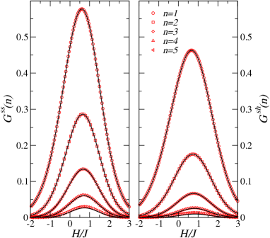
Figure 1: (Color on line) Correlation functions $G^{ss}(n)$ and $G^{sh}(n)$ along the ascending branch of the hysteresis loop for $z=2$ and $\Delta=4$. The simulation results (symbols) are compared to the predictions of Eqs. (12) (lines). Simulations were performed on random graphs with $N=10^{6}$ and the results were averaged over $1000$ disorder realizations.

The hysteresis loop in the 1D chain was calculated in Ref.S1996 . In this case, there are only three probabilities $p_{0},p_{1},p_{2}$ defined by Eq. (5), and from Eqs. (4) and (6) the magnetization along the ascending branch is simply given by

$$m=2\left[(1-P^{*})^{2}p_{0}+2P^{*}(1-P^{*})p_{1}+P^{*2}p_{2}\right]-1$$ (13)

with $P^{*}=p_{0}/(1-p_{1}+p_{0})$ (hereafter, to simplify the notation, the dependence of all quantities on the field $H$ is dropped). The results on the descending branch can be obtained by symmetry. The analytical calculation of the spin-spin correlation function $G^{ss}(n)$ was first considered in Ref.KFS2000 but the final expressions of $a$ and $b$ in Eq. (12a) are wrong (see Appendix A); the dependence on the distance $n$, however, is correctly given. Moreover, $G^{sh}(n)$ was not considered. On the other hand, the exact expressions of $G^{ss}(1)=\overline{S_{i}S_{i+1}}-m^{2}$ and $G^{sh}(0)=\overline{S_{i}h_{i}}$ were derived in Ref.ABCDDMZ2005 in order to compute the energy per spin along the hysteresis loop. The complete calculation that leads to Eqs. (12) is performed in Appendix A. In particular, we obtain

$$\lambda=p_{1}-p_{0}$$ (14)

as correctly found in Ref.KFS2000 . As shown in Fig. 1, Eqs. (12) are in excellent agreement with the results of numerical simulations performed on random graphs with $z=2$ (we also checked numerically that the expression of $G^{ss}(n)$ given in Ref.KFS2000 is not valid).

The two functions $G^{ss}(n)$ and $G^{sh}(n)$ are thus characterized by the same correlation length $\xi_{\lambda}=(-\ln\lambda)^{-1}=[-\ln(p_{1}-p_{0})]^{-1}$. However, $G^{ss}(n)$ is not a purely exponential function because of the prefactor $b(n-1)$. Remarkably, a similar behavior has been observed for the equilibrium RFIM in the very few cases where the correlation function $G^{ss}_{eq}(n)=\overline{<S_{i}S_{i\pm n}>}-\overline{<S_{i}>}\ \overline{<S_{i\pm n}>}$ has been calculated exactly. This is indeed the leading long-distance behavior observed at $T>0$ with the special random-field distribution (somewhat related to percolation) considered in Ref.GM1983 (in this model, however, the $T=0$ behavior is complicated and the correlation function behaves at long distance as an exponential divided by $n^{2}$LN1989 ). For the Gaussian distribution that we here consider, no analytical expression is available for generic values of $\Delta$ and $T$, but an exact result has been obtained in the universal regime where the random field and the temperature are both much smaller than the exchange couplingFLM2001 . For $H=0$, the leading long-distance behavior turns out to be also proportional to $n\exp{(-n/\xi_{eq})}$, where $\xi_{eq}=8J^{2}/(\pi^{2}\Delta)=(2/\pi^{2})L_{IM}$ and $L_{IM}$ is the Imry-Ma length that sets the typical size of the domains in the 1D chain at $T=0$IM1975 . This coincidence is noteworthy but it must emphasized that the full expression of $G^{ss}_{eq}(n)$ in this regime is much more complicated than the one described by Eq. (12a) (moreover, for $H\neq 0$, $G^{ss}_{eq}(n)$ decays as a sum of exponentials). The correlation length $\xi_{\lambda}$ along the hysteresis loop also behaves quite differently from $\xi_{eq}$ in the limit $\Delta\ll J$: it goes to the finite value $1/\ln(2)$ in zero applied field (as $H=0$ does not play any special role along the hysteresis loop) and grows like $\xi_{\lambda}\sim(\sqrt{\pi}J/\sqrt{2\Delta})\exp(J^{2}/2\Delta)$ for $H=J$, which is the value of the field for which the susceptibility $\partial m/\partial H$ is maximum.

An interesting consequence of Eq. (12a) is that the structure factor ${\hat{S}}(q)$ in the small-$q$ regime is a superposition of a Lorentzian and a Lorentzian-squared terms. By definition

$${\hat{S}}(q)=G^{ss}(0)+\sum_{n=1}^{\infty}[e^{iqn}+e^{-iqn}]G^{ss}(n)\ ,$$ (15)

and using

$$\sum_{-\infty}^{+\infty}e^{iql}\lambda^{|l|}=\frac{\sqrt{1-x^{2}}}{1-x\cos q}$$ (16)

with

$$x=\frac{2\lambda}{1+\lambda^{2}}\ ,$$ (17)

we obtain after simple algebra

$${\hat{S}}(q)=A+\frac{B}{1-x\cos q}+\frac{C}{[1-x\cos q]^{2}}$$ (18)

with

$$A =1-m^{2}+\frac{b-a}{\lambda}$$

$$B =\frac{(a-b)\sqrt{1-x^{2}}-b}{\lambda}$$

$$C =b\frac{1-x^{2}}{\lambda}\ .$$ (19)

The Lorentzian plus Lorentzian-squared structure that emerges from Eq. (18) in the small-$q$ regime is also found in the mean-field theory of the equilibrium RFIMKW1981 and is usually used to fit experimental data on random magnetic systems.

In contrast, the spin-random field correlation function $G^{sh}(n)$ is a pure exponential for $n\geq 1$ so that its Fourier transform simply reads

$$\hat{G}^{sh}(q)=[G^{sh}(0)-\frac{G^{sh}(1)}{\lambda}]+\frac{G^{sh}(1)}{\lambda}\frac{\sqrt{1-x^{2}}}{1-x\cos q}\ .$$ (20)

This yields

$$\hat{G}^{sh}(q=0)=G^{sh}(0)+\frac{2}{1-\lambda}G^{sh}(1)\ ,$$ (21)

and using the expression of the magnetization, Eq. (4), and Eqs. (B) and (B.2) for $G^{sh}(0)$ and $G^{sh}(1)$, one can check that the susceptibility sum-rule, $\hat{G}^{sh}(q=0)=\Delta(dm/dH)$, is indeed satisfied. Note that the $q$-independent term inside brackets in Eq. (20) is non-zero, which is a somewhat unusual feature (the constant term $A$ in Eq. (18) is also non-zero because Eq. (12a) is only valid for $n\geq 1$). As will be discussed in more detail in section III in the case of the Bethe lattice, this has a significant consequence for the matrix inverse of $G^{sh}$ (the so-called direct correlation function).

II.2 Bethe lattice

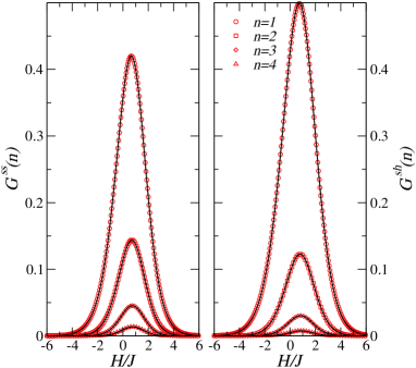
Figure 2: (Color on line ) Correlation functions $G^{ss}(n)$ and $G^{sh}(n)$ on a Bethe lattice with coordination number $z=3$ for $\Delta=9$ (the curves result from an average over $5000$ random graphs of size $N=10^{5}$). The simulation results (symbols) are compared to the predictions of Eqs. (12) (lines).

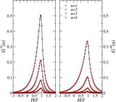
Figure 3: (Color on line) Same as Fig. 2 for $z=4$ and $\Delta=4$.

In principle, the probabilistic reasoning used in Appendix A for the one-dimensional chain can be extended to the case of the Bethe lattice with generic coordination number $z$. This is how the analytical expressions of $G^{ss}(1)$ and $G^{sh}(0)$ were derived in Ref.IOV2005 in order to compute the energy per spin along the hysteresis loop (thereby generalizing the 1D results of Ref.ABCDDMZ2005 ). These expressions are recalled in Appendix B where we also calculate $G^{ss}(2)$ and $G^{sh}(1)$. However, using the same method to derive the general expressions of $G^{ss}(n)$ and $G^{sh}(n)$ is unnecessarily complicated. Instead, one can simply exploit the fact that there is a unique path connecting a given pair of spins on a Bethe lattice so that the dependence of the correlation functions on the distance $n$ must be the same as in one-dimension (just like in nonrandom systems). This implies that Eqs. (12) are also valid for the Bethe lattice. Strictly speaking, we do not provide a demonstration of this assertion but it is fully supported by numerical simulations for small values of $n$, as illustrated in Figs. 2 and 3.

The analytical expression of $\lambda$ can then be obtained via the susceptibility sum-rule. Inserting Eq. (12b) in Eq. (11) yields

$$\Delta\frac{dm}{dH}=G^{sh}(0)+\frac{z}{1-(z-1)\lambda}G^{sh}(1)$$ (22)

so that

$$\lambda=\frac{1}{z-1}[1-z\frac{G^{sh}(1)}{\Delta\>dm/dH-G^{sh}(0)}]$$ (23)

Using Eqs. (4), (B) and (B.2), one can check that Eq. (14) is recovered for $z=2$.

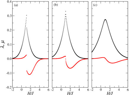
Figure 4: (Color on line) The quantities $\lambda(H)$ (top) and $\mu(H)$ (bottom) characterizing the exponential decay of the correlation and direct correlation functions, respectively, for $z=4$ and (a) $\Delta=2$, (b) $\Delta=\Delta_{c}\approx 3.173$, and (c) $\Delta=6$. In (a), below the critical disorder $\Delta_{c}$, $\lambda$ and $\mu$ jump discontinuously at the coercive field $H_{c}(\Delta)$. In (b), $\lambda\rightarrow(z-1)^{-1}=1/3$ at the critical field $H_{c}(\Delta_{c})=J$. Note that $\mu$ is significantly smaller than $\lambda$ in (c), above the critical disorder.

For $z\geq 4$ and $\Delta<\Delta_{c}(z)$, the magnetization jumps discontinuously at the coercive field $H_{c}(\Delta)$, which corresponds to a spinodal singularity where $dm/dH\rightarrow+\infty$DSS1997 ; CGZ2002 . As can be deduced from Eq. (22), this is due to the fact that $\lambda\rightarrow(z-1)^{-1}$, as illustrated in Fig. 4b for $z=4$. Therefore the correlation length $\xi_{\lambda}=(-\ln\lambda)^{-1}$ keeps a finite value at all $H$ and $\Delta$, including at the critical point. This is indeed the expected (and standard) behavior on the Bethe lattice where the divergence of the susceptibility is generated by the exponential growth of the number of sites at the distance $n$ (due to the hyperbolic-like geometry of the lattice) and is not associated to a divergence of the correlation length.

III Direct correlation functions

We now investigate the structure of the direct correlation functions (or one-particle irreducible functions, or else proper vertices in field-theoretic language) which (roughly speaking) are the matrix inverses of the correlation functions $G^{sh}_{ij}$ and $G^{sh}_{ij}$ (see Eqs. (24) and (46) below). As briefly mentioned in the introduction, the motivation for this calculation is that proper vertices may be simpler or at least shorter-ranged than the Green’s functions, and therefore can be used as the building blocks of approximate theories. For instance, in liquid-state theory, the direct correlation function $c(r)$, which is the matrix inverse of the pair correlation function $h(r)$ at equilibrium and is defined via the so-called Ornstein-Zernike (OZ) equation, is in general shorter-ranged than $h(r)$ (essentially having the range of the pair potential), irrespective of the thermodynamic stateHM2006 . This feature is the starting point of the successful integral equation approach to the structure and thermodynamics of simple liquids. For Ising spins on a lattice with nearest-neighbor interactions, it is also a reasonable approximation to assume that the matrix inverse of the spin-spin correlation function is zero for $n>1$note1 . This can been used to build a very accurate description of the three-dimensional Ising modelHS1977 and other spin modelsGKRT2001 , including in the presence of quenched disorderKRT1997 . More recently, a similar approximation has been proposed to obtain an analytical description of the hysteresis loop in the three-dimensional soft-spin random field model at $T=0$ RT2010 . It is therefore interesting to check whether the direct correlation functions on the Bethe lattice are indeed shorter-ranged than $G^{sh}$ and $G^{sh}$.

We first consider the function ${\bf C}^{sh}=\{C^{sh}_{ij}\}$ defined by the OZ equation $\sum_{k}C^{sh}_{ik}G^{sh}_{kj}=\delta_{ij}$, i.e.

$${\bf C}^{sh}=[{\bf G}^{sh}]^{-1}$$ (24)

where ${\bf G}^{sh}$ and ${\bf C}^{sh}$ are $N\times N$ matrices. As pointed out in the preceding section, $G^{sh}(n)$ is a pure exponential for $n>1$, but $G^{sh}(1)\neq\lambda G^{sh}(0)$. At first sight this is an innocuous feature but it has an important consequence for $C^{sh}(n)$. Indeed, as is well known (and is also shown below), if $G^{sh}(1)$ were equal to $\lambda G^{sh}(0)$ and therefore $G^{sh}(n)=\lambda^{n}G^{sh}(0)$ for all $n$, ${\bf C}^{sh}$ would be simply proportional to ${\bf A}$, the adjacency matrix of the lattice ($A_{ij}=1$ is the vertices $i$ and $j$ are connected and $0$ otherwise) and the range of $C^{sh}(n)$ would then be limited to the n.n. distance.

In order to solve the ‘Ornstein-Zernike’ equation (24), it is convenient to consider the simple random walk on the lattice where, at each time step, a particle jumps to any of the $z$ neighboring sites with probability $1/z$. Indeed, ${\bf G}^{sh}$ is directly related to the lattice Green function ${\bf F}(x)$ which is the probability generating function defined as (see e.g. Refs.G1994 ; MT1996 )

$$F_{ij}(x)=\sum_{\tau=0}^{\infty}x^{\tau}p^{\tau}_{ij}$$ (25)

where $p^{\tau}_{ij}$ is the probability that the particle starting at $i$ reaches $j$ after $\tau$ time steps. As is well known, one has

$${\bf F}(x)=({\bf I}-x{\bf M})^{-1}$$ (26)

where ${\bf M}=(1/z){\bf A}$. Since all sites are topologically equivalent, one can choose the origin of coordinates as the origin of the random walk and simply consider $F_{n}(x)=\sum_{\tau=0}^{\infty}x^{\tau}f_{\tau}(n)$ where $f_{\tau}(n)$ is the probability of being in the $n$th shell after $\tau$ time steps. By definition, $F_{0}(x)=F_{ii}(x)$ and $F_{n}(x)=c_{n}F_{ij}(x)$ where $i$ and $j$ are connected by $n\geq 1$ bonds (recall that $c_{n}=z(z-1)^{n-1}$). It can then be shownMT1996 that

$$F_{0}(x) =\frac{2(z-1)}{z-2+\sqrt{z^{2}-4(z-1)x^{2}}}$$

$$F_{n}(x) =c_{n}\Big{(}\frac{r(x)}{z-1}\Big{)}^{n}\ F_{0}(x)\ \ \ \mbox{for}\ n\geq 1$$ (27)

with

$$r(x)=\frac{z-\sqrt{z^{2}-4(z-1)x^{2}}}{2x}\ .$$ (28)

Using the identification

$$\lambda=\frac{r(x)}{z-1}\ ,$$ (29)

we readily see from Eq. (12b) that

$${\bf G}^{sh}=u{\bf F}(x)+v{\bf I}$$ (30)

with

$$u =\frac{G^{sh}(1)}{\lambda F_{0}(x)}$$

$$v =G^{sh}(0)-\frac{G^{sh}(1)}{\lambda}.$$ (31)

Note that Eq. (29) can also be written as

$$\lambda=\frac{F_{1}(x)}{xF_{0}(x)}=\frac{F_{0}(x)-1}{xF_{0}(x)}$$ (32)

which can be inverted to express $x$ as a function of $\lambda$,

$$x=\frac{z\lambda}{1+(z-1)\lambda^{2}}\ .$$ (33)

Therefore $x\rightarrow 1$ when $\lambda\rightarrow(z-1)^{-1}$ at the spinodal.

If $v$ were equal to $0$, one would simply have ${\bf C}^{sh}=[u{\bf F}]^{-1}=u^{-1}({\bf I}-x{\bf M})$ and $C^{sh}(n)$ would be zero for $n>1$, as stressed above. The matrix equation ${\bf C}^{sh}=[u{\bf F}+v{\bf I}]^{-1}$ is now easily solved:

$${\bf C}^{sh} =\frac{1}{u}[{\bf I}+\frac{v}{u}{\bf F}^{-1}(x)]^{-1}{\bf F}^{-1}(x)$$

$$=\frac{1}{u}[{\bf I}+\frac{v}{u}({\bf I}-x{\bf M})]^{-1}({\bf I}-x{\bf M})$$

$$=\frac{1}{u+v}[{\bf I}-\frac{vx}{u+v}{\bf M})]^{-1}({\bf I}-x{\bf M})$$

$$=\frac{1}{u+v}{\bf F}(x^{\prime})({\bf I}-x{\bf M})$$ (34)

where

$$x^{\prime}=\frac{v}{u+v}x\ .$$ (35)

This yields

$$C^{sh}_{ij}=\frac{1}{u+v}[F_{ij}(x^{\prime})-\frac{x}{z}\sum_{k/j}F_{ik}(x^{\prime})]$$ (36)

where $k$ is connected to $j$. Hence

$$C^{sh}(0) =\frac{1}{u+v}[F_{0}(x^{\prime})-\frac{x}{z}F_{1}(x^{\prime})]=-\frac{u}{v(u+v)}F_{0}(x^{\prime})+\frac{1}{v}$$

$$C^{sh}(1) =\frac{1}{u+v}[F_{1}(x^{\prime})-\frac{x}{z}(F_{0}(x^{\prime})+\frac{F_{2}(x^{\prime})}{z})]$$

$$=-\frac{u}{v(u+v)}\frac{F_{0}(x^{\prime})-1}{x^{\prime}}$$ (37)

and

$$C^{sh}(n) =\frac{1}{u+v}\Big{[}\frac{F_{n}(x^{\prime})}{c_{n}}-\frac{x}{z}[(z-1)\frac{F_{n+1}(x^{\prime})}{c_{n+1}}+\frac{F_{n-1}(x^{\prime})}{c_{n-1}}]\Big{]}$$

$$=\frac{1}{u+v}\frac{1}{c_{n}}\Big{[}F_{n}(x^{\prime})-\frac{x}{z}[F_{n+1}(x^{\prime})+(z-1)F_{n-1}(x^{\prime})]\Big{]}$$

$$=-\frac{u}{v(u+v)}\frac{F_{n}(x^{\prime})}{c_{n}}\ \ \mbox{for}\ \ n\geq 2$$ (38)

where we have used the recurrence relationsMT1996

$$F_{2}(x^{\prime}) =\frac{z}{x^{\prime}}F_{1}(x^{\prime})-zF_{0}(x^{\prime})$$

$$F_{n+1}(x^{\prime}) =\frac{z}{x^{\prime}}F_{n}(x^{\prime})-(z-1)F_{n-1}(x^{\prime})\ \ \mbox{for}\ n\geq 2\ .$$ (39)

Introducing

$$\mu=\frac{F_{0}(x^{\prime})-1}{x^{\prime}F_{0}(x^{\prime})}$$ (40)

which is equivalent to

$$x^{\prime}=\frac{z\mu}{1+(z-1)\mu^{2}}\ \ ,$$ (41)

we finally obtain

$$C^{sh}(0)=\frac{1}{u+v}F_{0}(x^{\prime})(1-\mu x)$$ (42)

and

$$C^{sh}(n)=-\frac{u}{v(u+v)}F_{0}(x^{\prime})\mu^{n}\ \ \mbox{for}\ n\geq 1\ .$$ (43)

For $z=2$, one has $F_{0}(x)=(1-x^{2})^{-1/2}$ and one can check that Eq. (43) is in agreement with the expression obtained by directly solving the OZ equation in Fourier space. One can also check that the following susceptibility sum-rule is satisfied,

$$\Delta\frac{dm}{dH}=[C^{sh}(0)+\frac{z}{1-(z-1)\mu}C^{sh}(1)]^{-1}\ .$$ (44)

We thus see from Eq. (43) that $C^{sh}(n)$ exhibits an exponential decay like $G^{sh}(n)$, but with a different correlation length $\xi_{\mu}=(-\ln|\mu|)^{-1}$. Moreover, since the sign of $v=G^{sh}(0)-G^{sh}(1)/\lambda$ depends on $H$, $\mu$ is not always positive (see Fig. 4) and there is a range of $H$ where the exponential decay is modulated by an oscillating sign. It turns out, however, that $\mu$ is significantly smaller than $\lambda$ in the weak-coupling (or large-disorder) regime, as illustrated in Fig. 4c, so that $C^{sh}(n)$ decreases rapidly with $n$. Indeed, expanding all quantities in powers of $J$, one finds that

$$G^{sh}(1)=\lambda G^{sh}(0)+O(J^{3})$$ (45)

so that $\mu=O(J^{3})$. Since $C^{sh}(1)=-J/\Delta+O(J^{2})$, this implies that $C^{sh}(2)=O(J^{4})$, $C^{sh}(3)=O(J^{7})$, etc… Therefore, setting $C^{sh}(n)=0$ for $n>1$ may be a reasonable approximation above the critical disorder (for instance, one has $J/\Delta_{c}\approx 0.315$ for $z=4$ at the critical disorder).

A similar calculation can be performed for the direct correlation function $C^{ss}(n)$ associated to the spin-spin correlation function $G^{ss}(n)$. It is defined via a second OZ equation

$${\bf C}^{ss}=-{\bf C}^{sh}{\bf G}^{ss}{\bf C}^{sh}$$ (46)

whose origin (in terms of a Legendre transform) is explained in Ref. RT2010 . After some involved algebra, we obtain

$$C^{ss}(n)=\mu^{n-1}[a^{\prime}+b^{\prime}(n-1)]$$ (47)

for $n\geq 1$, were $a^{\prime},b^{\prime}$ are functions of $H/J$ and $\Delta/J$ which are not detailed here for the sake of brevity. Hence $C^{ss}(n)$ has the same structure as $G^{ss}(n)$ with $\lambda$ replaced by $\mu$ (the fact that there is only one correlation length appearing in the final result and not two as could be expected from Eq. (46) is due to some remarkable cancellations occurring in the intermediate steps of the calculation). As a consequence, $C^{ss}(n)$ decreases rapidly with $n$ like $C^{sh}(n)$ (i.e. $C^{ss}(2)=O(J^{4})$, $C^{ss}(3)=O(J^{7})$, etc…), so that the n.n. approximation is also reasonable above $\Delta_{c}$.

IV Summary and conclusion

In this work we have determined the two-point spin-spin and spin-random field correlation (or Green’s) functions of the zero-temperature Gaussian RFIM on a Bethe lattice along the saturation hysteresis loop. This adds the model to the short list of nonequilibrium systems for which the correlation functions are analytically calculable. In the RFIM, these functions are not known at equilibrium, even in one dimension, except for very special random-field distributions or in the universal regime of very small disorder. We find that the two correlation functions decay exponentially with the distance with the same correlation length. This length remains finite at the disorder-induced critical point, which is the expected behavior on a Bethe lattice. The spin-spin correlation function also contains a prefactor proportional to the distance, so that the corresponding structure factor is a sum of a Lorentzian and a Lorentzian squared at small wavevector, just like in the mean-field description of the equilibrium RFIM. This gives some justification for using these simple functional forms to describe the data obtained in scattering experiments in RFIM-like systems (e.g. along the adsorption-desorption isotherms in the case of gases adsorbed in disordered porous solids). We also find that the direct correlation functions, which are the inverses of the correlation functions in the sense of matrices, have essentially the same analytic structure as the correlation functions, but with a different correlation length and a modulation of the sign (depending on the value of the applied field). This correlation length, however, is small, especially in the weak-coupling/large-disorder regime, and it is thus reasonable to assume that the range of the direct correlation functions is limited to the nearest-neighbor distance above the critical disorder. Although this ‘Ornstein-Zernike’ type of approximation breaks down in the vicinity of the critical pointnote2 , it may the starting point of an analytical description of the hysteresis loop in the three-dimensional RFIM, as developed recently for the soft-spin version of the modelRT2010 .

Appendix A Calculation of $G^{ss}(n)$ and $G^{sh}(n)$ in the one-dimensional chain

In this appendix, we present the calculation of the correlation functions $G^{ss}(n)$ and $G^{sh}(n)$ along the hysteresis loop in the 1D chain (specifically, along the ascending branch obtained by starting with a field $H$ large and negative). The correlations are obtained by generalizing the procedure used in Ref.S1996 to get the magnetization.

We first consider the spin-spin correlation function $G^{ss}(n)=\overline{S_{0}S_{n}}-\overline{S_{0}}^{2}$. As stressed in the main text, the calculation of $G^{ss}(n)$ was first considered in Ref.KFS2000 but the final expression is flawed. We therefore redo the whole calculation, closely following the reasoning and the notations of Ref.KFS2000 (note however that the calculation in Ref.KFS2000 is performed along the descending branch of the loop). By definition,

$$\overline{S_{0}S_{n}} =\sum_{S_{0},S_{n}}S_{0}S_{n}\Phi_{n}(S_{0},S_{n})$$

$$=\Phi_{n}(+,+)-\Phi_{n}(+,-)-\Phi_{n}(-,+)+\Phi_{n}(-,-)\ ,$$ (48)

where $\Phi_{n}(+,+)$ is the probability that spins at $0$ and $n$ are both up, and $\Phi_{n}(+,-),\Phi_{n}(-,+),\Phi_{n}(-,-)$ are defined analogously.

To calculate the probabilities $\Phi_{n}(S_{0},S_{n})$ we relax the spins in two steps (a spin is relaxed when it is aligned with its local field). In the first step, the spins $S_{0}$ and $S_{n}$ are kept down and the other spins can relax. In the second step, we also allow $S_{0}$ and $S_{n}$ to relax. The crucial point is that the final state does not depend on the order in which spins are relaxed.

In the first step, we need to compute the constrained probabilities $G_{n}(S_{1},S_{n-1})$ (not to be confused with the correlations functions) that the spins adjacent to $S_{0}$ and $S_{n}$ (see Fig. 5 for a schematic representation) are in the state $\{S_{1},S_{n-1}\}$.

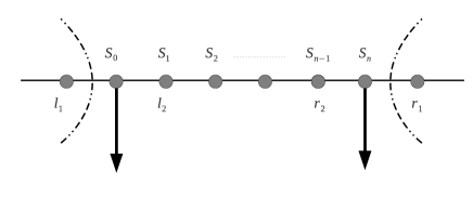
Figure 5: Schematic representation of the environment of the spins $S_{0}$ and $S_{n}$. In addition to the spin variables $S_{i}=\pm 1$, we also use the variables $l_{1}=(1+S_{-1})/2$, $l_{2}=(1+S_{1})/2$, $r_{2}=(1+S_{n-1})/2$, and $r_{1}=(1+S_{n+1})/2$ taking the values $0,1$.

A.1 Constrained probabilities $G_{n}(S_{1},S_{n-1})$

By definition,

$$G_{n}(S_{1},S_{n-1})=\sum_{S_{2}\ldots S_{n-2}}P(S_{1},S_{2}\ldots S_{n-2},S_{n-1})$$ (49)

where $P(S_{1},S_{2}\ldots S_{n-2},S_{n-1})$ is the probability of the configuration $\{S_{1},S_{2}\ldots S_{n-2},S_{n-1}\}$ when the spins $S_{0}$ and $S_{n}$ are pinned down and the spins between them are allowed to relax.

Carrying out the calculation as in Ref.KFS2000 , one easily derives the following recurrence relations for the constrained probabilities along the ascending branch of the hysteresis loop,

$$G_{n}(-,-) =(1-p_{0})G_{n-1}(-,-)+(1-p_{1})G_{n-1}(-,+)$$

$$G_{n}(+,-) =(1-p_{0})G_{n-1}(+,-)+(1-p_{1})G_{n-1}(+,+)\ .$$ (50)

Moreover $G_{n}(-,+)=G_{n}(+,-)$ by symmetry, and $G_{n}(+,+)$ is obtained via the sum-rule

$$G_{n}(-,-)+G_{n}(+,-)+G_{n}(-,+)+G_{n}(+,+)=1\ .$$ (51)

This gives the matrix equation

$${\bf G}_{n}={M}{\bf G}_{n-1}$$ (52)

where

$${\bf G}_{n}=\left[\begin{array}[]{c}G_{n}(-,-)\\ G_{n}(+,-)\\ G_{n}(+,+)\\ \end{array}\right]$$ (56)

and

$$M=\left[\begin{array}[]{lcr}1-p_{0}&1-p_{1}&0\\ 0&1-p_{0}&1-p_{1}\\ p_{0}&2p_{0}+p_{1}-1&2p_{1}-1\\ \end{array}\right]\ .$$ (60)

Hence ${\bf G}_{n}={M}^{n-1}{\bf G}_{1}$, with ${\bf G}_{1}\equiv\left[\begin{array}[]{c}1\\ 0\\ 0\\ \end{array}\right]$. We then change to the vector basisKFS2000

$$V=\left[\begin{array}[]{ccc}(1-P^{*})^{2}&+1&+1\\ P^{*}(1-P^{*})&-1&0\\ P^{*2}&+1&-1\\ \end{array}\right]$$ (61)

(recall that $P^{*}=p_{0}/(1-p_{1}+p_{0})$) in which the matrix $M$ takes the form

$$\tilde{M}=V^{-1}MV=\left[\begin{array}[]{ccc}1&0&0\\ 0&p_{1}-p_{0}&1-p_{1}\\ 0&0&p_{1}-p_{0}\\ \end{array}\right]$$ (62)

so that

$$\tilde{M}^{n-1}=\left[\begin{array}[]{ccc}1&0&0\\ 0&(p_{1}-p_{0})^{n-1}&(n-1)(1-p_{1})(p_{1}-p_{0})^{n-2}\\ 0&0&(p_{1}-p_{0})^{n-1}\\ \end{array}\right]\ .$$ (63)

To simplify the notation, we shift to the variables $l_{2}\equiv(1+S_{1})/2$ and $r_{2}\equiv(1+S_{n-1})/2$ that take the values $0,1$, and after some algebra we finally obtain

$$G_{n}(0,0) =(1-P^{*})^{2}+\big{[}P^{*}(1-P^{*})$$

$$+(n-1)P^{*}\frac{1-p_{1}}{p_{1}-p_{0}}+P^{*}\big{]}(p_{1}-p_{0})^{n-1}$$

$$G_{n}(1,0) =P^{*}(1-P^{*})-\big{[}P^{*}(1-P^{*})$$

$$+(n-1)P^{*}\frac{1-p_{1}}{p_{1}-p_{0}}\big{]}(p_{1}-p_{0})^{n-1}$$

$$G_{n}(1,1) ={P^{*}}^{2}+\big{[}P^{*}(1-P^{*})$$

$$+(n-1)P^{*}\frac{1-p_{1}}{p_{1}-p_{0}}-P^{*}\big{]}(p_{1}-p_{0})^{n-1}\ .$$ (64)

A.2 Calculation of $G^{ss}(n)$

To compute $\Phi_{n}(S_{0},S_{n})$ and then $G^{ss}(n)$ we now consider the second step where $S_{0}$ and $S_{n}$ are relaxed. We define $P(S_{0},S_{n}|l_{1},S_{1}\ldots S_{n-1},r_{1})$ as the probability of the state $\{S_{0},S_{n}\}$ under the condition that the state $\{l_{1},S_{1}\ldots S_{n-1},r_{1}\}$ has been reached after the first step (as indicated in Fig. 5, $l_{1}$ and $r_{1}$ describe the states of the spins $S_{-1}$ and $S_{n+1}$, respectively). Knowing these probabilities and the probability of all possible environments of $S_{0}$ and $S_{n}$ after the first relaxation step, we can write

$$\Phi_{n}(S_{0},S_{n}) =\sum_{l_{1}r_{1}}{P^{*}}^{l_{1}+r_{1}}\left(1-P^{*}\right)^{2-l_{1}-r_{1}}\sum_{S_{1}\ldots S_{n-1}}P(S_{1}\ldots S_{n-1})\sum_{S_{1}\ldots S_{n-1}}P(S_{1}\ldots S_{n-1})P(S_{0},S_{n}|l_{1},S_{1}\ldots S_{n-1},r_{1}).$$ (65)

If any of the spins $\{S_{1},\ldots,S_{n-1}\}$ is up the probability related to the second relaxation step is just a product of two independent terms. On the other hand, if all the spins $\{S_{1},\ldots,S_{n-1}\}$ are down, the expressions of the probabilities are more complicated since extra terms appear which account for the cases where the flip of $S_{0}$ (resp. $S_{n}$) triggers an avalanche which make all the spins $\{S_{1}...S_{n-1}\}$ to flip up, changing the environment or the state of $S_{n}$ (resp. $S_{0}$). This yields

$$\small P(-1,-1|l_{1},S_{1}\ldots S_{n-1},r_{1}) =(1-p_{l_{1}+l_{2}})(1-p_{r_{1}+r_{2}})$$

$$P(+1,-1|l_{1},S_{1}\ldots S_{n-1},r_{1}) =\left\{\begin{array}[]{lcr}p_{l_{1}+l_{2}}(1-p_{r_{1}+r_{2}})&\mbox{if}&\{S_{1}\ldots S_{n-1}\}\neq\{-1\dots-1\}\\ p_{l_{1}}(1-p_{r_{1}})-\left(\frac{p_{1}-p_{0}}{1-p_{0}}\right)^{n-1}p_{l_{1}}(p_{r_{1}+1}-p_{r_{1}})\mbox{\hskip 56.9055pt}&\mbox{if}&\{S_{1}\ldots S_{n-1}\}=\{-1\dots-1\}\\ \end{array}\right.$$ (68)

$$P(-1,+1|l_{1},S_{1}\ldots S_{n-1},r_{1}) =\left\{\begin{array}[]{lcr}(1-p_{l_{1}+l_{2}})p_{r_{1}+r_{2}}&\mbox{if}&\{S_{1}\ldots S_{n-1}\}\neq\{-1\dots-1\}\\ (1-p_{l_{1}})p_{r_{1}}-\left(\frac{p_{1}-p_{0}}{1-p_{0}}\right)^{n-1}(p_{l_{1}+1}-p_{l_{1}})p_{r_{1}}\mbox{\hskip 56.9055pt}&\mbox{if}&\{S_{1}\ldots S_{n-1}\}=\{-1\dots-1\}\\ \end{array}\right.$$ (71)

$$P(+1,+1|l_{1},S_{1}\ldots S_{n-1},r_{1}) =\left\{\begin{array}[]{lcr}p_{l_{1}+l_{2}}p_{r_{1}+r_{2}}&\mbox{if}&\{S_{1}\ldots S_{n-1}\}\neq\{-1\dots-1\}\\ p_{l_{1}}p_{r_{1}}+\left(\frac{p_{1}-p_{0}}{1-p_{0}}\right)^{n-1}\left[p_{l_{1}}(p_{r_{1}+1}-p_{r_{1}})+(p_{l_{1}+1}-p_{l_{1}})p_{r_{1}}\right]&\mbox{if}&\{S_{1}\ldots S_{n-1}\}=\{-1\dots-1\}\\ \end{array}\right.$$ (74)

where $l_{2}=(1+S_{1})/2$ and $r_{2}=(1+S_{n-1})/2$. Using Eqs. (49), (A.2), and the probability $(1-p_{0})^{n-1}$that all the spins $\{S_{1}\ldots S_{n-1}\}$ are down after the first relaxation step, we then obtain

$$\Phi_{n}(-,-) =\sum_{l_{1},r_{1}}P(l_{1},r_{1})$$

$$\times\Big{\{}\sum_{l_{2},r_{2}}G_{n}(l_{2},r_{2})(1-p_{l_{1}+l_{2}})(1-p_{r_{1}+r_{2}})\Big{\}}$$

$$\Phi_{n}(+,-) =\sum_{l_{1},r_{1}}P(l_{1},r_{1})\Big{\{}\sum_{l_{2},r_{2}}G_{n}(l_{2},r_{2})p_{l_{1}+l_{2}}(1-p_{r_{1}+r_{2}})$$

$$-(p_{1}-p_{0})^{n-1}p_{l_{1}}(p_{r_{1}+1}-p_{r_{1}})\Big{\}}$$

$$\Phi_{n}(-,+) =\sum_{l_{1},r_{1}}P(l_{1},r_{1})\Big{\{}\sum_{l_{2},r_{2}}G_{n}(l_{2},r_{2})(1-p_{l_{1}+l_{2}})p_{r_{1}+r_{2}}$$

$$-(p_{1}-p_{0})^{n-1}(p_{l_{1}+1}-p_{l_{1}})p_{r_{1}}\Big{\}}$$

$$\Phi_{n}(+,+) =\sum_{l_{1},r_{1}}P(l_{1},r_{1})\Big{\{}\sum_{l_{2},r_{2}}G_{n}(l_{2},r_{2})p_{l_{1}+l_{2}}p_{r_{1}+r_{2}}$$

$$+(p_{1}-p_{0})^{n-1}p_{l_{1}}(p_{r_{1}+1}-p_{r_{1}})$$

$$+(p_{1}-p_{0})^{n-1}(p_{l_{1}+1}-p_{l_{1}})p_{r_{1}}\Big{\}}.$$ (76)

where $P(l,r)\equiv{P^{*}}^{l+r}\left(1-P^{*}\right)^{2-l-r}$. One can check that the following exact relations are satisfied:

$$\Phi_{n}(+,-)= \Phi_{n}(-+)$$

$$\Phi_{n}(+,+)+2\Phi_{n}(+,-)+\Phi_{n}(-,-)= 1$$

$$\Phi_{n}(+,+)+\Phi_{n}(+,-)= \frac{1}{2}(m(H)+1)$$ (77)

where the magnetization $m(H)$ is given by Eq. (4).

In Fig. 6, Eqs. (A.2) are compared to simulation results in the case $n=4$. The excellent agreement confirms that the whole calculation is correct.

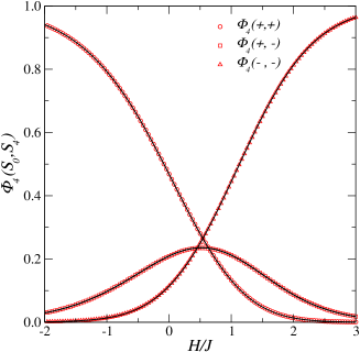
Figure 6: Probabilities $\Phi_{n}(S_{0},S_{4})$ along the ascending branch of the hysteresis loop for $z=2$ and $\Delta=4$. The simulation results (symbols) are compared to the predictions of Eqs. (A.2) (lines). Simulations were performed on random graphs with $N=10^{6}$ and the results were averaged over $1000$ disorder realizations.

Note that in Ref.KFS2000 it is stated that the probabilities $\Phi_{n}(S_{0},S_{n})$ are just linear combinations of the constrained probabilities $G_{n}$’s, without inhomogeneous terms. Eqs. (A.2) show that this is only true for $\Phi_{n}(--)$. Finally, inserting Eqs. (A.2) in Eq. (A) yields

$$\overline{S_{0}S_{n}} =\sum_{l_{1},r_{1}}P(l_{1},r_{1})\sum_{l_{2},r_{2}}G_{n}(l_{2},r_{2})(1-2p_{l_{1}+l_{2}})(1-2p_{r_{1}+r_{2}})$$

$$+4(p_{1}-p_{0})^{n-1}\sum_{l_{1},r_{1}}P(l_{1},r_{1})p_{l_{1}}(p_{r_{1}+1}-p_{r_{1}})\ .$$ (78)

A simpler expression is actually obtained by using Eqs. (A.2) to express $G^{ss}(n)$ in terms of $\Phi_{n}(-,-)$ only, as done in Ref.KFS2000 . This finally yields

$$G^{ss}(n) =4\Big{\{}\Phi_{n}(-,-)-[\frac{1-m(H)}{2}]^{2}\Big{\}}$$

$$=(p_{1}-p_{0})^{n-1}[a+b(n-1)]$$ (79)

with

$$a =4P^{*}(Q^{*}-P^{*})\left[2(1-P^{*})-P^{*}(Q^{*}-P^{*})\right]$$

$$b =4P^{*}(Q^{*}-P^{*})^{2}\frac{(1-p_{1})}{(p_{1}-p_{0})}\ .$$ (80)

For $z=2$ we recall that

$$P^{*} =\frac{p_{0}}{1-p_{1}+p_{0}}$$

$$Q^{*} =\frac{p_{1}-p_{1}^{2}+p_{0}p_{2}}{1-p_{1}+p_{0}}\ .$$ (81)

A.3 Calculation of $G^{sh}(n)=\overline{S_{0}h_{n}}$

We now consider the spin-random field correlation function

$$G^{sh}(n)\equiv\overline{S_{0}h_{n}}=\sum_{S_{0},S_{n}}\int dh_{n}S_{0}h_{n}\Phi_{n}(S_{0},S_{n},h_{n})$$ (82)

where $\Phi_{n}(S_{0},S_{n},h_{n})$ is the probability density that the two spins $S_{0}$ and $S_{n}$ are in the state $\{S_{0},S_{n}\}$ after full relaxation of the system, with the random field acting on the spin $S_{n}$ having a value within $(h_{n},h_{n}+dh_{n})$. The calculation of these probabilities is straightforward since we already have computed the probabilities $\Phi_{n}(S_{0},S_{n})$. We only need to restrict the integration of the random field distribution $\rho(h)$ over a range of $h$ compatible with the state of the spin $S_{n}$. This gives

$$\Phi_{n}(-,-,h_{n}) =\sum_{l_{1},r_{1}}P(l_{1},r_{1})\Big{\{}\sum_{l_{2},r_{2}}G_{n}(l_{2},r_{2})(1-p_{l_{1}+l_{2}})\rho(h_{n})\Theta[h_{n}<2(1-r_{1}-r_{2})J-H]\Big{\}}$$

$$\Phi_{n}(+,-,h_{n}) =\sum_{l_{1},r_{1}}P(l_{1},r_{1})\Big{\{}\sum_{l_{2},r_{2}}G_{n}(l_{2},r_{2})p_{l_{1}+l_{2}}\rho(h_{n})\Theta[h_{n}<2(1-r_{1}-r_{2})J-H]$$

$$-(p_{1}-p_{0})^{n-1}p_{l_{1}}\rho(h_{n})\Theta[2(1-r_{1}-1)J-H<h_{n}<2(1-r_{1})J-H]\Big{\}}$$

$$\Phi_{n}(-,+,h_{n}) =\sum_{l_{1},r_{1}}P(l_{1},r_{1})\Big{\{}\sum_{l_{2},r_{2}}G_{n}(l_{2},r_{2})(1-p_{l_{1}+l_{2}})\rho(h_{n})\Theta[h_{n}>2(1-r_{1}-r_{2})J-H]$$

$$-(p_{1}-p_{0})^{n-1}(p_{l_{1}+1}-p_{l_{1}})\rho(h_{n})\theta[h_{n}>2(1-r_{1})J-H]\Big{\}}$$

$$\Phi_{n}(+,+,h_{n}) =\sum_{l_{1},r_{1}}P(l_{1},r_{1})\Big{\{}\sum_{l_{2},r_{2}}G_{n}(l_{2},r_{2})p_{l_{1}+l_{2}}\rho(h_{n})\Theta[h_{n}>2(1-r_{1}-r_{2})J-H]$$

$$+(p_{1}-p_{0})^{n-1}p_{l_{1}}\rho(h_{n})\Theta[2(1-r_{1}-1)J-H<h_{n}<2(1-r_{1})J-H]$$

$$+(p_{1}-p_{0})^{n-1}(p_{l_{1}+1}-p_{l_{1}})\rho(h_{n})\Theta[h_{n}>2(1-r_{1})J-H]\Big{\}}$$ (83)

where $\Theta(.)$ is the characteristic function of the domain indicated by the argument (i.e. $1$ inside the domain and $0$ outside). Inserting in Eq.(82) yields

$$\overline{S_{0}h_{n}} =\int dh_{n}h_{n}\big{[}\Phi_{n}(+,-,h_{n})+\Phi_{n}(+,+,h_{n})-\Phi_{n}(-,-,h_{n})-\Phi_{n}(-,+,h_{n})\big{]}$$

$$=\sum_{l_{1},r_{1}}P(l_{1},r_{1})\sum_{l_{2},r_{2}}G_{n}(l_{2},r_{2})(2p_{l_{1}+l_{2}}-1)\int_{-\infty}^{+\infty}dh_{n}h_{n}\rho(h_{n})$$

$$+2(p_{1}-p_{0})^{n-1}\sum_{l_{1},r_{1}}P(l_{1},r_{1})(p_{l_{1}+1}-p_{l_{1}})\int_{2(1-r_{1})J-H}^{+\infty}dh_{n}h_{n}\rho(h_{n}),$$ (84)

and finally

$$\overline{S_{0}h_{n}} =2\Delta(p_{1}-p_{0})^{n-1}\left[\sum_{l_{1}}{P^{*}}^{l_{1}}(1-P^{*})^{1-l_{1}}(p_{l_{1}+1}-p_{l_{1}})\right]$$

$$\times\left[\sum_{r_{1}}{P^{*}}^{r_{1}}(1-P^{*})^{1-r_{1}}\rho\big{(}2(1-r_{1})J-H\big{)}\right].$$ (85)

Appendix B Calculation of $G^{ss}(2)$ and $G^{sh}(1)$ on the Bethe lattice.

In this Appendix we calculate $G^{ss}(2)$ and $G^{sh}(1)$ on a Bethe lattice with coordination number $z$. For completeness, we first recall the expressions of $G^{ss}(1)$ and $G^{sh}(0)$ obtained in Ref.IOV2005 :

$$G^{ss}(1)+m^{2}=1-4P^{*}+4P^{*}Q^{*}$$ (86)

where $Q^{*}$ is given by

$$Q^{*}=\sum_{k=0}^{z-1}{z-1\choose k}\left[P^{*}(H)\right]^{k}\left[1-P^{*}(H)\right]^{z-1-k}p_{k+1}(H)\ ,$$ (87)

and

$$G^{sh}(0) =2\Delta\sum_{k=0}^{z}{z\choose k}\left[p^{*}(H)\right]^{k}\left[1-p^{*}(H)\right]^{z-k}$$

$$\times\rho\big{(}(z-2k)J-H\big{)}\ .$$ (88)

We recall that $P^{*}$ (resp. $Q^{*}$) is the probability that, along the ascending branch of the loop, a spin is up given that a neighbor is forced to be down (resp. up).

B.1 Calculation of $G^{ss}(2)$

To compute the correlations between two spins $S_{1}$ and $S_{2}$ at the distance $n=2$ we consider a central spin $S_{0}$ and its $z$ neighbors $\{S_{1},\ldots S_{z}\}$ as depicted in Fig. 7a. By definition,

$$\overline{S_{1}S_{2}} =\sum_{S_{0},S_{1}\ldots S_{z}}S_{1}S_{2}P(S_{0},S_{1}\ldots S_{z})$$

$$=\sum_{S_{1},S_{2}}S_{1}S_{2}\big{[}\sum_{S_{3}\ldots S_{z}}P(-1,S_{1}\ldots S_{z})$$

$$+\sum_{S_{3}\ldots S_{z}}P(+1,S_{1}\ldots S_{z})\big{]}$$

$$=\sum_{S_{1},S_{2}}S_{1}S_{2}\left[P(-1,S_{1},S_{2})+P(+1,S_{1},S_{2})\right]$$ (89)

where $P(S_{0},S_{1},\ldots,S_{z})$ is the probability of having the configuration $\{S_{0},S_{1},\ldots,S_{z}\}$ when the system is fully relaxed.

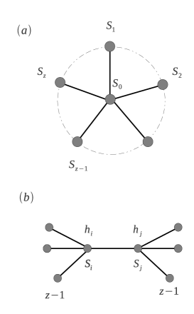
Figure 7: Schematic representation of the environment of (a) a single spin $S_{0}$ and (b) a pair of spins $S_{i}$ and $S_{j}$ .

By relaxing the spins in two steps, we obtain

$$P(-1,S_{1}\dots S_{z}) =\left[1-P^{*}\right]^{z-q}\left[P^{*}\right]^{q}(1-p_{q})$$ (90)

$$P(+1,S_{1}\ldots S_{z}) =\left[1-Q^{*}\right]^{z-q}\sum_{k=0}^{q}{q\choose k}$$

$$\times\left[Q^{*}-P^{*}\right]^{q-k}\left[P^{*}\right]^{k}p_{k}$$ (91)

where $q$ is the number of neighbors of $S_{0}$ that are up when the system is fully relaxed,

$$q=\frac{\sum_{j=1}^{z}S_{j}+z}{2}=0,1,\ldots z.$$ (92)

Eq. (90) is rather straightforward (recall that $P^{*}$ is the probability that a spin is up given that a neighbor is forced to be down). In Eq. (B.1), the summation accounts for all the different ways of having $S_{0}=1$ when $q$ neighbors are up, and the term in front of the summation accounts for the probability that $S_{0}$ has $z-q$ of his neighbors down if it is up.

Using Eqs. (90) and (B.1) we find

$$P(-1,S_{1},S_{2}) =\sum_{l=0}^{z-2}{z-2\choose l}\left[1-P^{*}\right]^{z-l-n}\left[P^{*}\right]^{l+n}(1-p_{l+n})$$

$$P(+1,S_{1},S_{2}) =\sum_{l=0}^{z-2}{z-2\choose l}\left[1-Q^{*}\right]^{z-l-n}\Big{[}\sum_{k=0}^{l+n}{l+n\choose k}$$

$$\times\big{[}Q^{*}-P^{*}\big{]}^{l+n-k}\left[P^{*}\right]^{k}p_{k}\Big{]}$$ (93)

where

$$n=\frac{S_{1}+S_{2}+2}{2}=0,1,2$$ (94)

We finally obtain the following expression for the correlations at the next-nearest neighbor distance

$$\overline{S_{1}S_{2}} =\sum_{n=0}^{2}(-1)^{n}{2\choose n}\sum_{l=0}^{z-2}{z-2\choose l}$$

$$\times\Bigg{\{}\left[1-P^{*}\right]^{z-l-n}\left[P^{*}\right]^{l+n}(1-p_{l+n})$$

$$+\left[1-Q^{*}\right]^{z-l-n}\left[\sum_{k=0}^{l+n}{l+n\choose k}\left[Q^{*}-P^{*}\right]^{l+n-k}\left[P^{*}\right]^{k}p_{k}\right]\Bigg{\}}$$ (95)

B.2 Calculation of $G^{sh}(1)$

To compute

$$G^{sh}(1)=\overline{S_{i}h_{j}}=\sum_{S_{i}}\int dh_{j}S_{i}h_{j}P(S_{i},h_{j})\ ,$$ (96)

we again relax the spins in two steps so to obtain

$$P(S_{i},h_{j}) =\sum_{l=0}^{z-1}{z-1\choose l}{P^{*}}^{l}(1-P^{*})^{z-1-l}$$

$$\times\sum_{r=0}^{z-1}{z-1\choose r}{P^{*}}^{r}(1-P^{*})^{z-1-r}P(S_{i},h_{j}|l,r),$$ (97)

where $P(S_{i},h_{j}|l,r)$ is the probability that the spin at $i$ is in the state $S_{i}$ after the second relaxation step, with the random field acting on $S_{j}$ having a value within $(h_{j},h_{j}+dh_{j})$, and under the condition that the environment of $S_{i}$ and $S_{j}$ is in the state $(l,r)$ after the first relaxation step (see Fig. 7b). As in Ref.IOV2005 , $l=1,\ldots,z-1$ (resp. $r=1,\ldots,z-1$) is the number of neighbors of $S_{i}$ ($S_{j}$) that are up, without taking into account $S_{j}$ (resp. $S_{i}$).

These probabilities are given by

$$P(-1,h_{j}|l,r) =\left\{\begin{array}[]{lrr}(1-p_{l})\rho(h_{j})&\mbox{if}&h_{j}<(z-2r)J-H\\ (1-p_{l+1})\rho(h_{j})&\mbox{if}&h_{j}>(z-2r)J-H\end{array}\right.$$ (100)

$$P(+1,h_{j}|l,r) =\left\{\begin{array}[]{lrr}p_{l}\rho(h_{j})\mbox{\hskip 25.6073pt}&\mbox{if}&h_{j}<(z-2r)J-H\\ p_{l+1}\rho(h_{j})\mbox{\hskip 25.6073pt}&\mbox{if}&h_{j}>(z-2r)J-H\ .\end{array}\right.$$ (103)

Inserting these expressions in Eq. (B.2) and after some algebra we finally obtain

$$G^{sh}(1) =2\Delta\left[\sum_{l=0}^{z-1}{z-1\choose l}{P^{*}}^{l}(1-P^{*})^{z-1-l}(p_{l+1}-p_{l})\right]$$

$$\times\left[\sum_{r=0}^{z-1}{z-1\choose r}{P^{*}}^{r}(1-P^{*})^{z-1-r}\rho((z-2r)J-H)\right]\ .$$ (104)

For $z=2$ and $n=1$, one can check that this equation gives back Eq. (A.3).

References

- (1) J. P. Sethna, K. A. Dahmen, and O. Perkovíc in The Science of Hysteresis, edited by G. Bertotti and I. Mayergoyz, Acedemic Press, Amsterdam (2006).
- (2) J. P. Sethna, K. A. Dahmen, S. Kartha, J. A. Krumhansl, B. W. Roberts, and J. D. Shore, Phys. Rev. Lett. 70, 3347 (1993).
- (3) F. Detcheverry, E. Kierlik, M. L. Rosinberg, and G. Tarjus, Phys. Rev. E 72, 051506 (2005).
- (4) F. Bonnet, T. Lambert, B. Cross, L. Guyon, F. Despetis, L. Puech, and P. E. Wolf, Europhys. Lett. 82, 56003 (2008).
- (5) D. Dhar, P. Shukla, and J.P. Sethna, J. Phys. A 30, 5259 (1997); S. Sabhapandit, P. Shukla, and D. Dhar, J. Stat. Phys. 98, 103 (2000); P. Shukla, Phys. Rev. E 63, 027102 (2001).
- (6) F. Colaiori, A. Gabrielli, and S. Zapperi, Phys. Rev. B 65, 224404 (2002).
- (7) M. J. Alava, V. Basso, F. Colaiori, L. Dante, G. Durin, A. Magni, and S. Zapperi, Phys. Rev. B 71, 064423 (2005).
- (8) X. Illa, J. Ortín, and E. Vives, Phys. Rev. B 71, 184435 (2005); X. Illa, P. Shukla, and E. Vives, Phys. Rev. B, 73 092414 (2006).
- (9) H. Ohta and S. Sasa, Euro. Phys. Lett. 90, 27008 (2010).
- (10) M.L. Rosinberg and G. Tarjus, J. Stat. Mech. P12011 (2010).
- (11) For a recent review, see E. Hoinkis, Part. Part. Syst. Charact. 21, 80 (2004).
- (12) F. Detcheverry, E. Kierlik, M. L. Rosinberg, and G. Tarjus, Phys. Rev. E 73, 041511 (2006).
- (13) J. C. Kimball, H. L. Frisch, and L. Senapati, Physica A 279, 151 (2000).
- (14) See e.g. T. Natterman, Spin glasses and random fields (World Scientific, Singapore, 1998).
- (15) P. Shukla, Physica A 233, 235 (1996).
- (16) G. Grinstein and D. Mukamel, Phys. Rev. B 27, 4503 (1983).
- (17) J.M. Luck and Th.M. Nieuwenhuizen, J. Phys. A 22, 2151 (1989); see also J.M. Luck, Systèmes Désordonnés Unidimensionnels (Saclay Aléa, 1992). On the other hand, in the random one-dimensional lattice-gas studied by Y. Fonk and H. J. Hilhorst, J. Stat. Phys. 49, 1235 (1987), the correlation function at also displays the prefactor.
- (18) D. Fisher, P. Le Doussal, and C. Monthus, Phys. Rev. E 64, 066107 (2001). In this work, the nonequilibrium dynamics of the RFIM chain after a quench from a random initial condition (e.g. a high temperature state) is studied via an asymptotically exact real space renormalization group analysis. As a byproduct, the equilibrium quantities at low temperature are obtained in the long time limit, at the end of the renormalization procedure.
- (19) Y. Imry and S. K. Ma, Phys. Rev. Lett. 35, 1399 (1975).
- (20) H. S. Kogon and D. J. Wallace, J. Phys. A: Math. Gen. 14 L527 (1981).
- (21) T.P. Handford, F-J Perez-Reche, and S. N. Taraskin, arXiv:cond-mat/1106.3424v1.
- (22) J. P. Hansen and I. R. McDonald, Theory of simple liquids (Academic Press, 2006).
- (23) However this type of ‘Ornstein-Zernike’ approximation implies that the small-wavevector behavior of the correlation function is regular so that the anomalous dimension is zero.
- (24) J. S. Hoye and G. Stell, J. Chem. Phys. 67, 439 (1977); Mol. Phys. 52, 1071 (1984); D. Pini and G. Stell, Phys. Rev. Lett. 77, 996 (1996); D. Pini, G. Stell, and R. Dickman, Phys. Rev. E 57, 2862 (1998).
- (25) S. Grollau, E. Kierlik, M.L. Rosinberg and G. Tarjus, Phys. Rev. E 63, 041111 (2001); S. Grollau, M.L. Rosinberg and G. Tarjus, Physica A 296, 460 (2001).
- (26) E. Kierlik, M. L. Rosinberg, and G. Tarjus, J. Stat. Phys. 89, 215 (1997); ibid 94, 805 (1999); ibid 100, 423 (2000).
- (27) A. Giacometti, J. Phys. A: Math. Gen. 28, L13 (1995).
- (28) C. Monthus and C. Texier, J. Phys. A: Math. Gen. 29, 2399 (1996).
- (29) This is especially true in the three-dimensional RFIM since the anomalous dimensions and associated to the connected and disconnected correlation functions, respectively, are rather large.