Dragging two-dimensional discrete solitons by moving linear defects

Abstract

We study the mobility of small-amplitude solitons attached to moving defects which drag the solitons across a two-dimensional (2D) discrete nonlinear-Schrödinger (DNLS) lattice. Findings are compared to the situation when a free small-amplitude 2D discrete soliton is kicked in the uniform lattice. In agreement with previously known results, after a period of transient motion the free soliton transforms into a localized mode pinned by the Peierls-Nabarro potential, irrespective of the initial velocity. However, the soliton attached to the moving defect can be dragged over an indefinitely long distance (including routes with abrupt turns and circular trajectories) virtually without losses, provided that the dragging velocity is smaller than a certain critical value. Collisions between solitons dragged by two defects in opposite directions are studied too. If the velocity is small enough, the collision leads to a spontaneous symmetry breaking, featuring fusion of two solitons into a single one, which remains attached to either of the two defects.

I Introduction

The discrete nonlinear Schrödinger (DNLS) equations constitute a vast class of systems which are profoundly interesting in their own right, and serve as important physical models for nonlinear optics PhysRep , matter waves in Bose-Einstein condensates (BECs) Smerzi , and in other contexts Panos . In particular, soliton solutions to the DNLS equation in one, two, and three dimensions (1D, 2D, and 3D) represent fundamental localized modes in discrete media. Experimentally, 1D and 2D quasi-discrete solitons have been created in nonlinear optical systems of several types, see a comprehensive review in Ref. PhysRep .

Local defects are important ingredients of DNLS models. They are interesting as additional dynamical elements of the lattices Panos , and have direct physical realizations. In particular, they may describe various strongly localized structures in photonic crystals defect0 , such as nanocavities defect1 , micro-resonators defect2 , and quantum dots defect3 . In the context of BEC, local defects can be easily created and used for manipulating the condensate by means of focused laser beams. This technique has made it possible to create optical tweezers for trapping and controllable transfer of condensates by moving optical traps tweezers . A scheme for nonlinear optical tweezers that can extract solitons from a linear reservoir was proposed too Humberto .

In a more general context, controllable transport of solitons in periodic and quasiperiodic media, including the ultimate case of discrete lattices, plays an important role in various applications, see Refs. transport and references therein. Many attempts have been made to devise a simple way of transferring solitons from one position to another with minimal losses. In particular, dragging gap solitons in BEC, embedded into an optical lattice, by a moving defect to which the soliton is attached, was proposed as a means of the transport in Ref. BBK . Recently, manipulations of a BEC vortex by a localized impurity representing a focused laser beam was considered in Ref. Panos1 .

The subject of the present work is the dragging of discrete solitons in 2D lattices by an attractive defect which plays the role of the mover. The defect is shaped as a Gaussian of a finite width. After introducing the model and recapitulating some relevant results for static trapped modes in Sect. 2, we consider moving solitons in Sect. 3. First, the problem of the immobility of free 2D DNLS solitons is briefly revisited, and then new results are reported for the transfer of solitons by the moving attractive defect. Both simple rectilinear dragging routes, and more sophisticated ones, in the form of square, rhombic, and circular closed trajectories, are considered. It is concluded that the trapped solitons may survive the dragging over an indefinitely long distance, if the dragging velocity does not exceed a certain critical value. The paper is concluded by Sect. 4.

II The model and stationary solutions

II.1 The formulation

We consider the following model based on the 2D DNLS equation with a local defect:

$$i\dot{u}_{n,m}+J\Delta_{2}u_{n,m}+V_{n,m}(t)u_{n,m}+\sigma|u_{n,m}|^{2}u_{n,m}=0,$$ (1)

where the overdot stands for the time derivative, $\Delta_{2}u_{n,m}\equiv u_{n,m+1}+u_{n,m-1}+u_{n+1,m}+u_{n-1,m}-4u_{n,m}$ is the 2D discrete Laplacian, the coupling constant of the lattice will be fixed by scaling, $J\equiv 1$, and $\sigma>0$ is the coefficient of the on-site self-attraction. Discrete function $V_{n,m}$ account for the linear defect, taken in the form as a Gaussians profile,

$$V_{n,m}(t)=v\exp\left\{-\left[\left(n-n(t)\right)^{2}+\left(m-m(t)\right)^{2}\right]/\Delta^{2}\right\},$$ (2)

with respective strength $v$, width $\Delta$, and coordinates of the (moving) center, $n(t)$ and $m(t)$. In this notation, positive and negative strengths correspond to the attractive and repulsive defect, respectively.

Looking for stationary solutions in the case of the quiescent defect, with $m(t)=n(t)\equiv 0$ in Eq. (2),

$$u_{n,m}=U_{n,m}\exp(-i\omega t),$$ (3)

we arrive at the nonlinear eigenvalue problem,

$$\omega U_{n,m}+\Delta_{2}U_{n,m}+V_{n,m}U_{n,m}+\sigma|U_{n,m}|^{2}U_{n,m}=0,$$ (4)

for real frequency $\omega$ and the profile of the stationary discrete mode, $U_{m,n}$, which may be complex, in the general case. In the absence of the defect, the linearized version of Eq. (4) gives rise to the dispersion relation for linear modes $U_{m,n}\sim\exp\left(ikm+iqn\right)$,

$$\omega=4\left[\sin^{2}\left(k/2\right)+\sin^{2}\left(q/2\right)\right],$$ (5)

which features the phonon band, $0\leq\omega\leq 8$. Above and below the band, full nonlinear equation (4) gives rise to nonlinear modes, described by respective curves $N(\omega)$, with $N=\sum_{m,n}|u_{m,n}|^{2}$ being the norm (power) of the mode. The important difference between 2D and 1D settings is that, in the latter case, the fundamental single-peak mode (alias the Sievers-Takeno discrete soliton) admits the limit of $N\rightarrow 0$, while all the 2D solitons are bounded by a critical norm, $N_{\mathrm{cr}}$, below which they do not exist Panos . Accordingly, an abrupt delocalization (decay) of discrete 2D solitons was predicted in the case when the inter-site coupling constant exceeds a certain critical value Bishop . It is worthy to mention that, introducing a defect with the linear and nonlinear components and varying their strengths, or the lattice coupling constant, in time (in the spirit of the “soliton management” techniques book ), one can change the critical norm, $N_{\mathrm{cr}}$, and thus control the transition to the delocalization we .

II.2 Existence curves for stationary solitons and stability

Curves $N(\omega)$ for the discrete solitons obtained from numerical solutions of Eq. (4), based on the continuation from the anti-continuum limit [the one corresponding to $J=0$ in Eq. (1)], using the standard Newton’s iteration routine, are displayed in Fig. 1, in the presence and in the absence of the defect. In panel 1(a) we compare three curves: the black one for the case of $\sigma=1$ without the defect, and the blue and red curves for $\sigma=1$ and $\sigma=0.25$ with the defect of amplitude $v=1$ and width $\Delta=1$ [the red curve is obtained from the blue one by rescaling of the norm, in order to get a curve crossing the black one in a vicinity of $\omega\rightarrow 0$, see Fig. 1(b)]. In the defect-free lattice, a family of stable solitons (in agreement with the Vakhitov-Kolokolov (VK) criterion, it obeys condition $dN/d\omega<0$ Panos ) can be found in the region of $-\infty<\omega<\omega_{\mathrm{cr}}\approx-1$. In this region, the discrete soliton is tightly localized, being immobile, due to the strong pinning to the underlying Peierls-Nabarro potential Panos . The Peierls-Nabarro potential becomes weak for broad small-amplitude discrete solitons corresponding to $\omega\rightarrow 0$. Note that the introduction of the positive defect can significantly reduce or completely suppress the instability region, as shown by the blue and red curves in Fig. 1(a) where only a small segment of the existence curve in the interval of $-0.58<\omega<-0.52$ remains unstable. Note also that the attractive defect removes the lower existence bound for the 2D discrete solitons, $N_{\mathrm{cr}}$, as the soliton goes over into a linear defect mode in the limit of $N\rightarrow 0$.

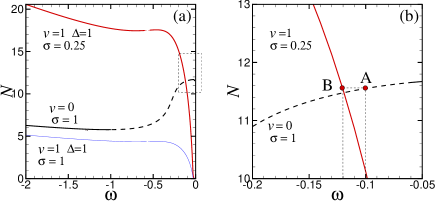
Figure 1: (Color online) (a) The existence curves for on-site symmetric solitons in the defect-free lattice ($v=0$, the black line), and in the presence of the quiescent defect (2) with $v=1$ and $\Delta=1$, for different values of the nonlinearity coefficient: $\sigma=1$ and $\sigma=0.25$ (the blue and red lines, respectively). The dashed part of the black curve corresponds to unstable solitons in the uniform lattice. Panel (b) shows a zoom of the dashed box from (a). Points A and B correspond to the solitons with frequencies $\omega_{A}=-0.1$ and $\omega_{B}=-0.17$, and equal norms, $N_{A}=N_{B}$.

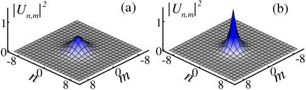
Figure 2: Profiles of unstable and stable discrete solitons, which correspond, respectively, to points A and B of the existence curves in Fig. 1(b).

According to the previous analysis, at small $|\omega|$ initially unstable discrete solitons in the uniform lattice may be stabilized by switching the attractive defect on Panos ; we . To keep the norm of the soliton constant in this case, simultaneously with introducing the defect we decrease the strength of the nonlinearity. As a result, we obtain the existence curve shown in red in Fig. 1(a), which features intersection with the original black line in the region of $|\omega|\ll 1$. The stabilization corresponds to the transition from point A to B in Fig. 1(b), which follows the increase of the strength of the defect from $v=0$ to $v=1$ and reduction of the strength of the nonlinear coefficient from $\sigma=1$ to $\sigma=0.25$. We have checked numerically that the transition between these two configurations could be performed even instantaneously in time, leading to a very small radiation loss. Examples of the profiles of the discrete solitons found without and with the defect are displayed in Fig. 2. Both solutions have the same norm, while solitons A and B belong, respectively, to the unstable and stable branches of the existence curves, cf. Fig. 1.

III Moving solitons

III.1 Dynamics of discrete solitons in the uniform lattice

Proceeding to the consideration of traveling solitons, it is first relevant to recapitulate basic results concerning the ballistic motion of kicked solitons in the uniform lattice. We kick the discrete soliton by taking the initial condition as $U_{n,m}=U_{n,m}^{(0)}\exp\left[-i(c_{n}n+c_{m}m)/2\right]$, where $U_{n,m}^{(0)}$ is stationary configuration (3), and vector $(c_{n},c_{m})$ determines the strength and direction of the initial impulse. Figure 3 demonstrates that the broad small-amplitude soliton from Fig. 2(a), if kicked in the $n$ direction by the impulses of different strengths, $c_{n}=0.1$, $0.2$, and $0.5,$ is transformed into a tightly localized peak, which keeps nearly the entire initial norm and comes to the halt at a site with coordinate $n_{f}$. Note also that the initial broad soliton was unstable, while the final tall peak (with almost the same norm) represents a stable soliton, as per the black curve in Fig. 1.

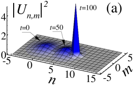
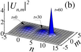
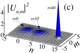
Figure 3: Snapshots of the discrete soliton initially kicked in the horizontal direction ($c_{m}=0$), are shown at different times. The initial profile is taken from Fig. 2(a). Parameters of the kick and the coordinate of the final pinned site, $n_{f}$, are $c_{n}=0.1$, $n_{f}=7$ in (a); $c_{n}=0.2$, $n_{f}=9$ in (b), and $c_{n}=0.5$, $n_{f}=12$ in (c).

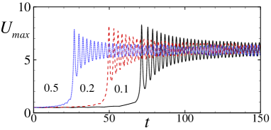
Figure 4: (Color online) The evolution of the peak density for three different values of the kick: $c_{n}=0.1$ (solid black), $c_{n}=0.2$ (dashed red), and $c_{n}=0.5$ (dotted blue). Other parameters are as in Fig. 3.

This and other simulations corroborate the known fact that, under the action of the kick applied in any direction relative to the underlying 2D lattice, the broad 2D DNLS soliton starts to move, but eventually stops after having traveled a finite distance (on the contrary to the 1D DNLS model, where the kicked soliton may travel indefinitely long 1D ; Panos ). The harder the initial shove $c_{n}$, the longer distance $n_{f}$ is passed by the discrete soliton before the stoppage (cf. Fig.3). However, an excessively strong kick induces strong perturbations in the shape of the soliton, under the action of which it starts to radiate, leading to a significant loss of the norm. In Fig. 4, the peak density of the moving soliton, determined as $U_{\max}=\max(|u_{n,m}|^{2})$, is displayed for different strengths of the initial kick. It is seen that, after coming to the halt, the initially broad soliton transforms into a highly localized mode whose amplitude features gradually fading oscillations. Similar results were obtained for the propagation of the discrete soliton initially kicked in the diagonal direction, with $c_{n}=c_{m}$.

Thus, persistent motion of solitons in the uniform 2D DNLS lattice is impossible. This may be explained by the fact that, in the continual limit, the cubic self-focusing leads to the collapse of solitons; in the discrete setting, this implies the formation of tightly localized tall peaks, which are strongly pinned to the lattice, being therefore immobile. On the other hand, it is known that motile 2D solitons are possible in discrete media with weaker nonlinearities, which do not lead to the collapse in the continual limit, viz., saturable Johansson and quadratic chi2 on-site nonlinear terms. In the 2D lattice with the combination of self-focusing cubic and defocusing quintic terms (this combination of the nonlinearities does not give rise to the collapse in the continuum medium either), the kicked soliton may perform a long run, but eventually it comes to a halt, because of radiation losses CQ .

III.2 Dragging the discrete solitons by the moving defect along the linear trajectory

Forced motion of solitons attached to moving defects is the central topic of this work. To demonstrate a typical realization of this scenario, we take the initial soliton from Fig. 2(b), and drive the defect in the lattice plane along a rectilinear rout: $n(t)=n_{s}+c_{n}t,$ $m(t)=m_{s}+c_{m}t$, where $c_{n}$ and $c_{m}$ are the velocities in the $n$ and $m$ directions. A set of typical examples is displayed in Fig. 5, for dragging the discrete soliton in the $n$ direction with different velocities, $c_{n}=0.1,$ and $0.5$. This figure demonstrates that the soliton can be transferred, virtually without any loss of the norm, over indefinitely long distances, if the velocity, which is applied instantaneously, is small enough, allowing the soliton to permanently adjust itself, in an adiabatic manner, to the positions passed in the course of the motion [Fig. 5(a)]. In more quantitative terms, this may be explained by the comparison of the dragging velocity with the vectorial group velocity produced by dispersion relation (5): $\mathbf{v}\equiv\partial\omega/\partial\left\{k,q\right\}=2\left\{\sin k,\sin q\right\}$. If the dragging velocity is not small enough in comparison with the group velocity, the adiabatic adjustment of the moving soliton is not possible, and the soliton will be destroyed by the emission of radiation waves escaping at the group velocity.

To further illustrate peculiarities of the dynamics of the driven soliton, its peak density is displayed in Fig. 6, as a function of the rescaled time, for different dragging velocities. The oscillations correspond to transformations between on-site (maximum peak density) and off-site (minimum peak density) configurations of the discrete soliton. At small dragging velocities, the total norm remains practically constant after a small initial loss of the norm due to the radiation, while the large velocity ($c_{n}=0.5$ in Fig. 6) causes a significant initial loss. In the latter case, the subsequent dynamics shows conservation of the total norm. Similar results (not displayed here) have been obtained for the driven motion of the soliton along the lattice diagonal. We do not aim here to exactly identify the critical velocity for the transition from the movable solitons to immovable ones, as the transition is somewhat fuzzy, going through an intermediate region where the radiation loss suddenly starts to increase with the growth of the driving velocity.

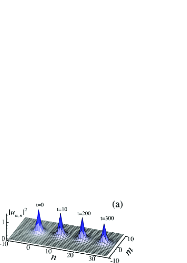
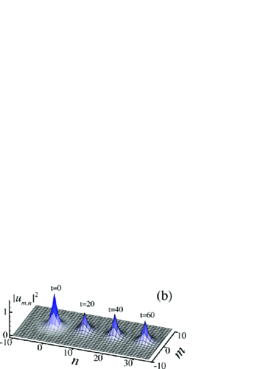
Figure 5: Snapshots of the discrete soliton, dragged by the moving defect, at different times. The initial profile, as well as parameters of the defect, are the same as in Fig. 2(b) ($v=\Delta=1$). The velocity of the defect is $c_{n}=0.1$ in (a), and $c_{n}=0.5$ in (b). The other component of the velocity is absent, $c_{m}=0$.

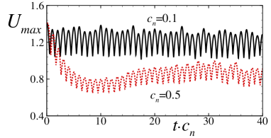
Figure 6: (Color online) The evolution of the peak density for two different values of the dragging velocity: $c_{n}=0.1$ (solid black), $c_{n}=0.5$ (dashed red). Other parameters are the same as in Fig. 5.

III.3 Dragging the soliton along closed trajectories

To demonstrate more sophisticated kinetic effects, in Fig. 7 we display dragging the soliton along a closed trajectory formed by four segments aligned with bonds of the lattice. Typical results are also displayed in Fig. 8 for the driven motion along a closed route formed by four diagonal segments. Figures 7 and 8 suggest that, in the case of the abrupt changes in the direction of the driven motion, the velocity of the dragging defect is a crucial parameter, leading to strong losses at large velocities. Indeed, the comparison of Figs. 7(b) 8(c) to Fig. 5(b) demonstrates that relatively high velocities produce a much more destructive effect on the solitons dragged along the closed trajectories than on their linearly driven counterparts. On the other hand, for sufficiently small velocities [$c_{n}=$ $0.1$ in Figs. 7(a) and 8(a)], the soliton can be dragged along complex routes in the virtually intact form. Continuing the study in this direction, we have also considered driven circular motion of the soliton, as shown in Fig. 9, where the discrete soliton is safely dragged along the ring trajectory with radius $R=15$ and angular velocity $0.01/\pi$.

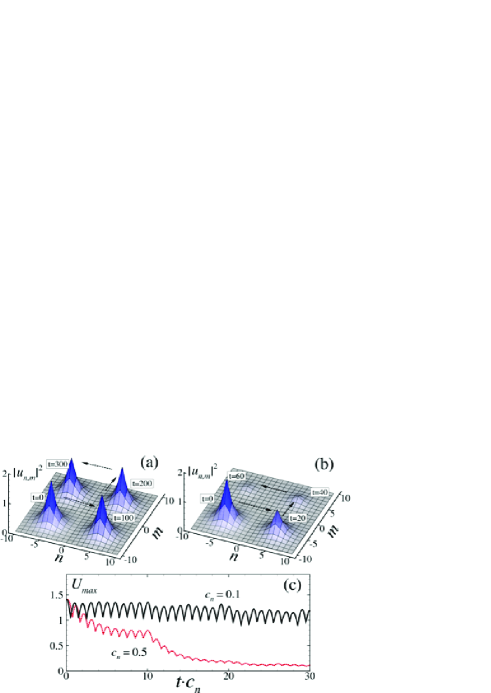
Figure 7: The same as in Fig. 5, but for dragging the soliton along the square formed by the lattice axes. Here the corresponding velocities along the $n$ and $m$ directions are $|c_{n}|=|c_{m}|=0.1$ in (a) and $|c_{n}|=|c_{m}|=0.5$ in (b). In panel (c), the time evolution of the peak density $U_{\max}$ for both cases is shown.

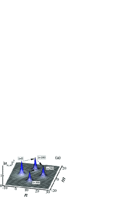
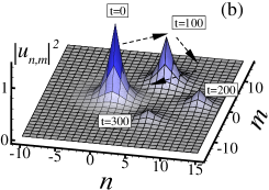
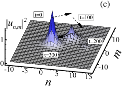
Figure 8: The same as in Figs. 7(a) and (b), for dragging the soliton along the rhombus formed by diagonals of the lattice. Here $|c_{n}|=|c_{m}|=0.1$, $0.3$, and $0.5$, in (a), (b) and (c), respectively.

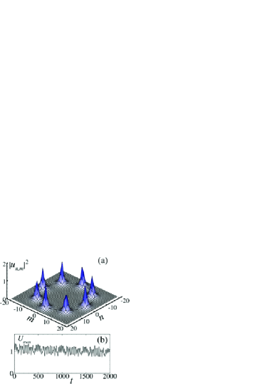
Figure 9: Dynamics of the discrete soliton with initial profile taken from Fig. 2(a) and initially placed at position $(n,m)=(R,0)$ with $R=15$. The defect moves along the circular trajectory: $n_{d}=R\cos(0.01t/\pi)$ and $m_{d}=R\sin(0.01t/\pi)$. The snapshots are shown with interval $t=250$. In panel (b), the evolution of the peak density is shown.

III.4 Collisions between discrete solitons dragged by defects

Another natural problem is collisions between defect-dragged solitons. First, we consider the head-on collision between identical solitons dragged toward each other. Colliding, they temporarily merge into a “lump” with the double norm, roughly adjusted to the defect with doubled strength. Continuing the simulations and monitoring attempts of the subsequent evolution of the merged lump, we observed two different scenarios, depending on the velocity of the dragging. If the velocity is higher then some critical value, after the separation of the two defects the lump splits back into two solitons, which are tantamount to those existing before the collision, see Fig. 10.

The collision dynamics drastically changes if the velocity is smaller than the critical value, see Fig. 11. Just before the collision, but when the two defects are still well separated in space (in the present case, at $t\approx 750$), one observes a symmetry breaking in the distribution of the local power (density) in the merging lump, which becomes unstable against oscillations of the total norm between the two defects. At the time of the collision, almost the same behavior occurs as in the previous example pertaining to the higher velocity. However, after the separation of the defects, the lump does not split, staying attached, as a single soliton, to one defect and moving with it, while the other defect remains “bare”, as seen in Fig. 11(c).

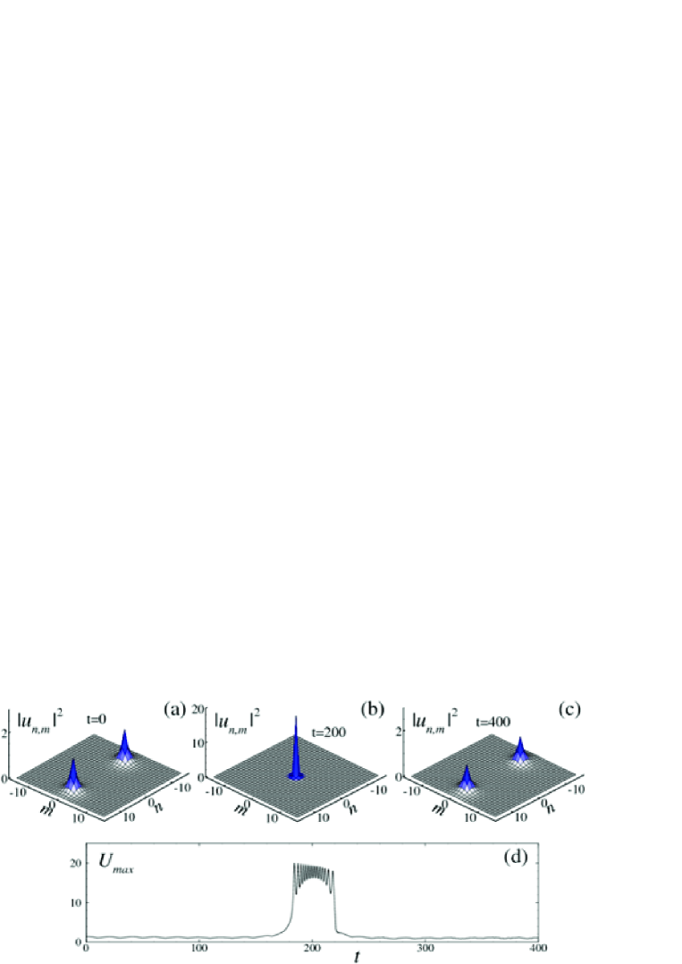
Figure 10: The collision between two discrete solitons dragged by defects with velocities $|c_{n}|=0.05$. Panels (a), (b) and (c) display profiles of the solitons in the initial state, at the collision moment, and in the final state, respectively. In panel (d) the respective evolution of the peak density is presented. The initial solitons are taken from Fig. 1(b).

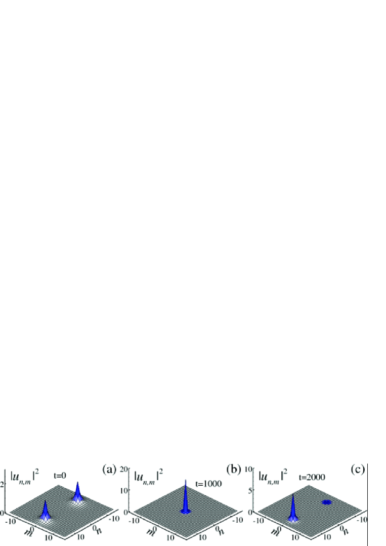
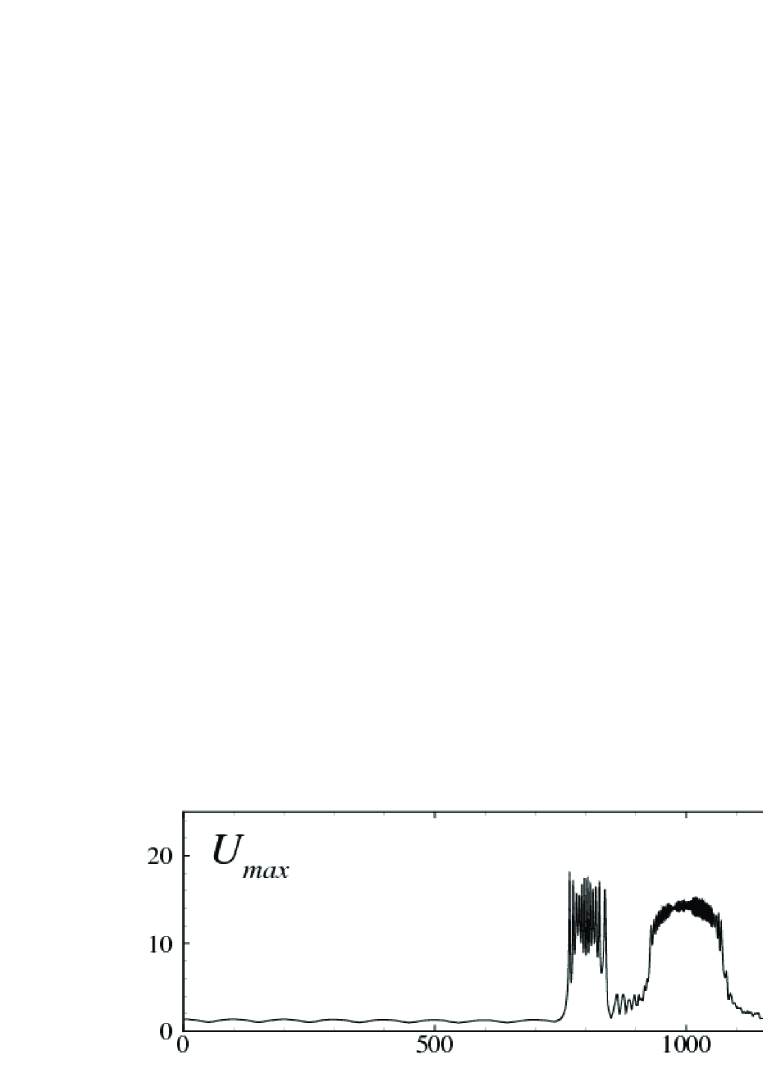
Figure 11: The same as in Fig.10, but for velocities $|c_{n}|=0.01$.

The symmetry breaking in the head-on collisions of the dragged solitons can be explained by the consideration of a linear-stability problem. To this end, we calculated the existence curves for static symmetric and asymmetric modes trapped by a pair of defects separated by different constant distances, and checked the linear stability of those modes, taking perturbed solutions as $u_{n,m}=\exp(-i\omega t)[U_{n,m}+a_{n,m}\exp(\lambda t)+b_{n,m}\exp(\lambda^{\ast}t)]$, where $\lambda$ is an eigenvalue, $U_{n,m}$ is the unperturbed stationary solution, and $a_{n,m},b_{n,m}$ are small perturbations. The so found unstable symmetric (dashed lines) and stable asymmetric (solid lines) families of the solutions are presented in Fig. 12(a), with the distance between the defects being $\delta=8$ (black) and $10$ (red) sites (the corresponding existence curves are practically overlapping). In Fig. 12(b) dependences of the most unstable eigenvalues (the real part of $\lambda$) on frequency $\omega$ for the symmetric configurations with different distances between the defects from Fig. 12(a) are presented. One can conclude that the symmetric configuration is unstable against small perturbations (with the most unstable eigenvalue substantially diminishing with the increase of the separation between the defects). Although this instability pertains to the symmetric lumps supported by the pair of immobile defects, it provides an explanation to the instability of the merged symmetric lump also in the case of the slowly colliding defects.

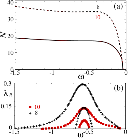
Figure 12: (Color online) (a) Existence curves for the families of symmetric (upper lines) and asymmetric (lower lines) discrete solitons supported by a symmetric pair of the defects. Solid and dashed portions of the curves correspond to stable and unstable solutions. Black and red lines (mostly overlapping) pertain to the configurations with the distance between the defects fixed to be $\delta=8$ and $10$ sites, respectively. (b) The frequency dependence of the real part of the two most unstable eigenvalues for the symmetric solutions from (a). The black (+) and red ($\blacksquare$) symbols correspond to the distances between the defects $\delta=8$ and $10$, respectively.

As mentioned above, the symmetry breaking occurs between the colliding solitons driven by the slowly moving defects. This fact can be explained by comparing the time necessary for the development of the instability of the lump produced by the collision and the collision time. The time of the mutual passage of the solitons attached to rapidly moving defects is smaller than the time required for the onset of the instability. In this case, the collision is quasi-elastic, and it does not cause the breaking of the symmetry between the solitons, while for smaller velocities the collision time is sufficient for the development of the instability and ensuing symmetry breaking, which may eventually transform the two solitons into one, pinned to a single defect. Similar arguments were previously used to explain the transition from quasi-elastic collisions to symmetry-breaking ones in several models supporting 1D solitons in continual models Javid .

We have also considered the collision of solitons with a mismatch in direction $m$ perpendicular to the velocities (the “aiming parameter”), $\xi=|m_{1}-m_{2}|$, where $m_{j}$ defines the initial coordinate of the $j$-th soliton in the direction of $m$. In particular, for the same small velocities as in Fig. 11, with two different values of the mismatch, $\xi=8$ and $\xi=10$, the results are shown in Fig. 13. It is seen that the character of the collision can be controlled by varying the mismatch, cf. Ref. George , where the collisions were simulated between 2D solitons in the framework of a continual dissipative equation.

IV Conclusion

In this work, we have elaborated a scenario for the controlled transfer of 2D discrete solitons through the DNLS lattice. The main obstacle to the transport is the fact that 2D solitons in the uniform DNLS system cannot move persistently under the action of an initial kick, being always braked by the underlying Peierls-Nabarro potential. Nevertheless, we have demonstrated that a relatively broad soliton can be dragged over indefinitely large distances, with virtually zero loss, by the moving attractive defect, provided that the dragging velocity does not exceed a critical value. This is qualitatively explained by the comparison of the dragging velocity with the group velocity of the linear waves propagating in the uniform lattice. The stable driven motion is possible in any direction, as well as along complex routes with corners, and along circular trajectories; however, the critical velocity is lower in the latter cases. Collisions between solitons dragged by two solitons in opposite directions were considered too, with the conclusion that the two solitons spontaneously merge into a single one, which stays attached to either moving defect, if the collision velocity is small enough.

These scenarios can be implemented (and used for various applications) in the following form: a quiescent soliton may be prepared in the uniform 2D lattice, then the local attractive defect(s) may be induced [for instance, by laser beam(s) illuminating the corresponding BEC], effectively converting the free solitons into defect modes; next, the mode(s) may be transferred to a new position, as described above, and, eventually, the laser beam(s) may be switched off. Eventually, free solitons may be transferred according to this protocol, in the medium where these solitons are not motile by themselves.

The analysis presented above may be naturally extended in various directions, including the transfer of vortex solitons vortex (in the latter case, the trapping defect must be wide enough, for a sufficient overlap with the vortex; in fact, the defect itself may have a vortical structure). A challenging generalization would be to develop a similar scenario for discrete solitons in 3D lattices, which may also be realized in terms of BEC.

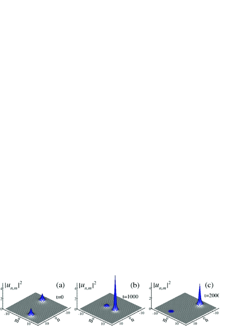
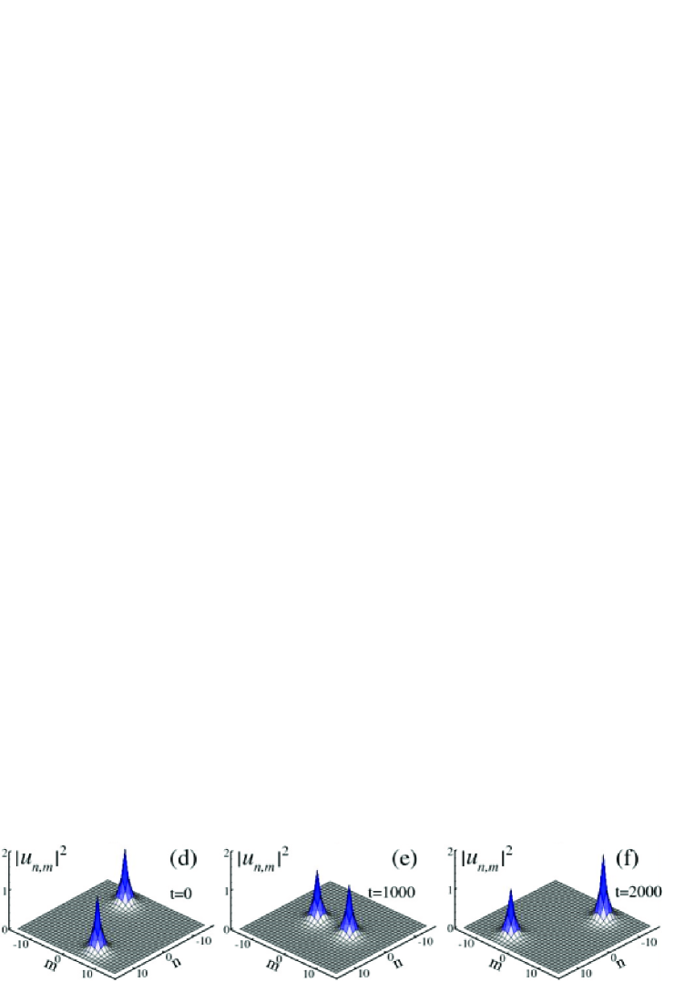
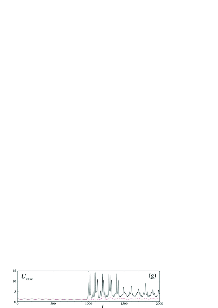
Figure 13: Color online) The collision with finite mismatch $\xi$. The snapshots in (a)-(c) and (d)-(f) correspond to $\xi=8$ and $\xi=10$, respectively. In panel (g), the respective evolution of the peak density is shown for $\xi=8$ (solid black) and $\xi=10$ (dashed red).

References

- (1) F. Lederer, G. I. Stegeman, D. N. Christodoulides, G. Assanto, M. Segev, and Y. Silberberg, Phys. Rep. 463, 1 (2008).
- (2) A. Trombettoni and A. Smerzi, Phys. Rev. Lett. 86, 2353 (2001); F. Kh. Abdullaev, B. B. Baizakov, S. A. Darmanyan, V. V. Konotop, and M. Salerno, Phys. Rev. A 64 043606 (2001); G.L. Alfimov, P. G. Kevrekidis, V. V. Konotop, and M. Salerno, Phys. Rev. E 66, 046608 (2002).
- (3) P. G. Kevrekidis, editor, The Discrete Nonlinear Schrödinger Equation: Mathematical Analysis, Numerical Computations, and Physical Perspectives (Springer: Berlin and Heidelberg, 2009).
- (4) T. Hattori, N. Tsurumachi, and H. Nakatsuka, J. Opt. Soc. Am. B 14, 348 (1997).
- (5) Y. Akahane, T. Asano, B. S. Song, and S. Noda, Nature 425, 944 (2003).
- (6) R. Colombelli, K. Srinivasan, M. Troccoli, O. Painter, C. F. Gmachl, D. M. Tennant, A. M. Sergent, D. L. Sivco, A. Y. Cho, and F. Capasso, Science 302, 1374 (2003).
- (7) H. Nakamura, Y. Sugimoto, K. Kanamoto, N. Ikeda, Y. Tanaka, Y. Nakamura, S. Ohkouchi, Y. Watanabe, K. Inoue, H. Ishikawa, and K. Asakawa,Opt. Exp. 12, 6606 (2004).
- (8) T. L. Gustavson, A. P. Chikkatur, A. E. Leanhardt, A. Gorlitz, S. Gupta, D. E. Pritchard, and W. Ketterle, Phys. Rev. Lett. 88, 020401 (2001); A. E. Leanhardt, A. P. Chikkatur, D. Kielpinski, Y. Shin, T. L. Gustavson, W. Ketterle, and D. E. Pritchard, ibid. 89, 040401 (2002); V. Boyer, R. M. Godun, G. Smirne, D. Cassettari, C. M. Chandrashekar, A. B. Deb, Z. J. Laczik, and C. J. Foot, Phys. Rev. A 73, 031402 (2006).
- (9) A. V. Carpentier, J. Belmonte-Beitia, H. Michinel, and Rodas-Verde, J. Mod. Opt. 55, 2819 (2008).
- (10) N. J. Zabuski, Computer Physics Communications 5, 1 (1973); O. M. Braun and Y. S. Kivshar, Phys. Rep. 306, 2 (1998); B. A. Malomed, Z. H. Wang, P. L. Chu, and G. D. Peng, J. Opt. Soc. Am. B 16, 1197 (1999); R. G. Scott, A. M. Martin, S. Bujkiewicz, T. M. Fromhold , N. Malossi, O. Morsch, M. Cristiani, E. Arimondo, Phys. Rev. A 69, 033605 (2004); V. Ahufinger, A. Sanpera, P. Pedri, L. Santos, and M. Lewenstein, ibid. A 69, 053604 (2004); B. Freedman, G. Bartal, M. Segev, R. Lifshitz, D. N. Christodoulides, and J. W. Fleischer, Nature 440, 1166 (2006).
- (11) V.A. Brazhnyi, V.V. Konotop, V. M. Pérez-García, Phys. Rev. Lett. 96, 060403 (2006); Phys. Rev. A 74, 023614 (2006).
- (12) M. C. Davis, R. Carretero-González, Z. Shi, K. J. H. Law, P. G. Kevrekidis, and B. P. Anderson, Phys. Rev. A 80, 023604 (2009).
- (13) G. Kalosakas, K. Ø. Rasmussen, and A. R. Bishop, Phys. Rev. Lett. 89, 030402 (2002).
- (14) B. A. Malomed, Soliton Management in Periodic Systems (Springer: New York, 2006).
- (15) V. A. Brazhnyi and B. A. Malomed, Phys. Rev. E, 83, 016604 (2011).
- (16) D. B. Duncan, J. C. Eilbeck, H. Feddersen, and J. A. D. Wattis, Physica D 68, 1 (1993); S. Flach and K. Kladko, ibid. 127, 61 (1999); S. Flach, Y. Zolotaryuk, and K. Kladko, Phys. Rev. E 59, 6105 (1999); M. J. Ablowitz, Z. H. Musslimani, and G. Biondini, ibid. 65, 026602 (2002); I. E. Papacharalampous, P. G. Kevrekidis, B. A. Malomed, and D. J. Frantzeskakis, Phys. Rev. E 68, 046604 (2003).
- (17) R. A. Vicencio and M. Johansson, Phys. Rev. E. 73, 046602 (2006); U. Naether, R. A. Vicencio, and M. Johansson, Phys. Rev. E 83, 036601 (2011).
- (18) H. Susanto, P. G. Kevrekidis, R. Carretero-González, B. A. Malomed, and D. J. Frantzeskakis, Phys. Rev. Lett. 99, 214103 (2007).
- (19) C. Chong, R. Carretero-González, B. A. Malomed, and P. G. Kevrekidis, Physica D 238, 126 (2009).
- (20) J. Atai and B. A. Malomed, Phys. Rev. E 62, 8713 (2000); 64, 066617 (2001); Phys. Lett. A 298, 140 (2002); 342, 404 (2005).
- (21) G. Wainblat and B. A. Malomed, Physica D 238, 1143 (2009).
- (22) B. A. Malomed and P. G. Kevrekidis, Phys. Rev. E 64, 026601 (2001).