The Bragg regime of the two-particle Kapitza-Dirac effect

Abstract

We analyze the Bragg regime of the two-particle Kapitza-Dirac arrangement, completing the basic theory of this effect. We provide a detailed evaluation of the detection probabilities for multi-mode states, showing that a complete description must include the interaction time in addition to the usual dimensionless parameter $w$. The arrangement can be used as a massive two-particle beam splitter. In this respect, we present a comparison with Hong-Ou-Mandel-type experiments in quantum optics. The analysis reveals the presence of dips for massive bosons and a differentiated behavior of distinguishable and identical particles in an unexplored scenario. We suggest that the arrangement can provide the basis for symmetrization verification schemes.

PACS: 03.75.Dg; 42.50.Xa; 61.05.J-

1 Introduction

The Kapitza-Dirac proposal [1] provides a beautiful demonstration of the diffraction of massive particles by standing light waves. The proposal has been realized experimentally for atoms and electrons [2, 3, 4, 5, 6].

More recently, it has been suggested that additional effects could be present when we move from one- to two-particle massive systems interacting with the optical diffraction grating [7]. In this type of arrangement two different dynamics take place simultaneously. On the one hand, the particles interact with the optical wave generating diffraction patterns. On the other hand, if the two particles are identical, the exchange effects must also be taken into account. The resultant joint dynamics shows a much richer behavior.

As it is well-known [8], there are two regimes in the Kapitza-Dirac effect, diffraction and Bragg scattering. In [7] the first one was studied for two-particle systems. Here, we complete the basic analysis of the two-particle Kapitza-Dirac effect by considering two-particle Bragg scattering.

As we did in [7], we consider separately single- and multi-mode states. In contrast with [7], where we only gave a qualitative description of the second ones, we present here a simple model of the problem that allows for a detailed quantitative evaluation of the detection probabilities in the multi-mode case. Our model takes into account the dependence of the width of the window of modes that can be scattered on the duration of the interaction [9, 10]. Because of this dependence, the probabilities of transmission and reflection of multi-mode states must be expressed in terms of the interaction time, in addition to the dimensionless parameter $w$, which is the only parameter present in the case of single-mode states.

Although the Bragg scattering of massive particles has been extensively studied, specially in BEC, there are some aspects of the two-particle problem that still deserve attention. In particular, the behavior of massive particles in Hong-Ou-Mandel (HOM)-type experiments [11] remains rather unexplored. As these experiments have played an important role in quantum optics it seems necessary to analyze its massive counterpart. In this respect, it has been many times suggested in the literature the possibility of using the Bragg regime of the Kapitza-Dirac effect as a basis for massive beam splitters [10, 12]. This is a natural choice because it generates two possible exit paths for the particles, just as a beam splitter. As a simple extension of these ideas, it is natural to think of the two-particle Bragg scattering as a serious candidate for the implementation of massive two-particle beam splitters.

Several results emerge from our analysis: (i) We show that, just as for photons, one can observe dips in the case of massive bosons. (ii) We have, as in quantum optics [13, 14], that the behavior of distinguishable and identical particles is the same if the parallel momenta of the two particles are equal. However, if the two particles are in different multi-mode states we can observe different behaviors. This is a previously not considered scenario, which deserves attention. (iii) Finally, we shall propose a possible application of the arrangement. The two-particle Bragg scattering could be used to test the (anti)symmetrization of the wave functions of pairs of identical particles.

The plan of the paper is as follows. In Sect. 2 we briefly review the fundamentals of the Bragg regime in the Kapitza-Dirac effect, and we discuss the different situations present in its two-particle extension. We devote Sects. 3 and 4 to the evaluation of the detection probabilities for, respectively, single- and multi-mode states. The possibility of using the two-particle Kapitza-Dirac arrangement as a massive two-particle beam splitter is presented in the Discussion where, in addition to recapitulate on the main results of the paper, we compare our approach with HOM-type experiments.

2 General considerations

The Bragg scattering is the relevant process for thick standing waves with weak associated potentials. When these two conditions are fulfilled the diffraction can only take place for some particular angles, the Bragg angles. This behavior contrasts with that observed for thin waves, where diffraction occurs for any angle of incidence and many different diffraction orders can be reached. On the other hand, if the potential is strong, we have coherent channeling.

The theory of one-particle Bragg scattering by a standing light wave can be found in [8]. In this reference there is also an excellent discussion of the physical and mathematical differences between the Bragg and diffraction regimes. We denote by $k_{L}$ the wave number of the optical grating, usually a laser beam. When the particle is incident on the grating at the Bragg angle, $\hbar k_{L}/p$ with $p$ the total momentum of the particle, the energy and momentum are conserved. In addition, the particles incident exactly at the first order of the grating (the momentum parallel to the grating equal to $\hbar k_{L}$) can be scattered into the $-1st$ order with a momentum change $2\hbar k_{L}$. Moreover, the transitions to other orders are forbidden.

From a more mathematical point of view, the (first-order) Bragg angle $\theta$ is given by the expression $\lambda=d_{L}\sin\theta$, where $\lambda$ is the de Broglie wavelength of the particles and $d_{L}=\lambda_{L}/2$ is the periodicity of the light beam. The interaction of the particle with the grating is ruled by the potential $V=V_{0}\cos^{2}k_{L}x$, with $x$ denoting the coordinate parallel to the grating. As usual, the solution of the quantum equation of evolution is obtained by introducing wave functions of the form $\psi(x,X)=\sum_{n}c_{n}\exp(i(nk_{L}x+KX))$, with $X$ the coordinate perpendicular to the grating and $K$ the initial wave number in that axis (which does not change because the interaction along it is null). In the Bragg regime, being the incident wave function in the state $n=1$, the final state of the particle can only be $n=\pm 1$ with coefficients [8]:

$$c_{+}=e^{-i\epsilon\tau}\cos w\;;\;c_{-}=-ie^{-i\epsilon\tau}\sin w\;;\;w=\frac{V_{0}\tau}{4\hbar}$$ (1)

where $\tau$ denotes the duration of the interaction, $\epsilon=\hbar k_{L}^{2}/2m$, and $c_{+}=c_{1}$ and $c_{-}=c_{-1}$. The above equation shows an oscillatory behavior of the probabilities of finding the particle in each of the orders $n=\pm 1$ as a function of $V_{0}\tau$.

Note that although the incident $x$-component of the momentum of the particle is fixed to $\hbar k_{L}$, varying $K$ we can have different Bragg’s angles.

When we have two incident particles we have a wider range of possibilities. They are depicted in Fig. 1:

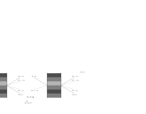
Figure 1: Two particles incident on a standing light wave. The full and dashed lines represent, respectively, particles with momenta perpendicular to the light wave $K$ and $K^{\prime}$. The parallel momenta $\pm k$ are $\pm k_{L}$ (or values very close to them, see the multi-mode section).

The part $(I)$ of the figure corresponds to the case in which both particles arrive to the grating with the same momentum in the direction parallel to the light beam, $k_{L}$ (in the multi-mode realm we must also consider values of $k$ very close but not equal to $k_{L}$, see Sect. 4). As signaled before, taking different momenta in the perpendicular axis we can have different Bragg’s angles (the angle between the path and the normal to the grating). On the other hand, the part $(II)$ of the figure represents the situation where the parallel momenta of the two particles are opposite.

In the case $(I)$ the wave functions of the two particles after the interaction are

$$\psi_{k_{L},K}(x,X)=c_{+}e^{i(k_{L}x+KX)}+c_{-}e^{i(-k_{L}x+KX)}$$ (2)

and

$$\psi_{k_{L},K^{\prime}}(y,Y)=c_{+}e^{i(k_{L}y+K^{\prime}Y)}+c_{-}e^{i(-k_{L}y+K^{\prime}Y)}$$ (3)

where $y$ and $Y$ denote the coordinates of the other particle.

From these expressions one can derive, as in [7], the wave functions in momentum space. Instead, we move to the more concise brackets formalism, where we have $|k_{L},K>_{1}=c_{+}|k_{L}>_{1}|K>_{1}+c_{-}|-k_{L}>_{1}|K>_{1}$ and $|k_{L},K^{\prime}>_{2}=c_{+}|k_{L}>_{2}|K^{\prime}>_{2}+c_{-}|-k_{L}>_{2}|K^{\prime}>_{2}$, with the subscripts $1$ and $2$ denoting the two particles.

When the two particles are distinguishable the complete states are $|I>_{dis}=|k_{L},K>_{1}|k_{L},K^{\prime}>_{2}$ and $|II>_{dis}=|k_{L},K>_{1}|-k_{L},K^{\prime}>_{2}$ (where now $|-k_{L},K^{\prime}>_{2}=c_{+}|-k_{L}>_{2}|K^{\prime}>_{2}+c_{-}|k_{L}>_{2}|K^{\prime}>_{2}$). In contrast, if the particles are identical the wave function must be (anti)symmetrized, that is, $|I>=N|k_{L},K>_{1}|k_{L},K^{\prime}>_{2}\pm N|k_{L},K^{\prime}>_{1}|k_{L},K>_{2}$ and $|II>=N|k_{L},K>_{1}|-k_{L},K^{\prime}>_{2}\pm N|-k_{L},K^{\prime}>_{1}|k_{L},K>_{2}$, where the upper sign holds for bosons and the lower one for fermions. $N$ is the normalization coefficient, which will be determined later.

We assume that the particles are in the same (or symmetric) spin and electronic states. Thus, as done above, the spatial part of the wave function must be symmetric for bosons and antisymmetric for fermions. By simplicity, the spin and electronic variables can be dropped from all the expressions. The extension to antisymmetric spin or electronic states is straightforward.

3 Single-mode states

This section is devoted to the simple case of single-mode states. With this simplification it is easy to illustrate the properties of the system. Later, in the next section, we move to the more realistic case of multi-mode states.

3.1 Distinguishable particles

In order to later compare with identical particles, we assume both distinguishable particles to be characterized by the same $c_{\pm}$ coefficients (both masses to be equal). Using the explicit expression for $|I>_{dis}$, the probabilities are easily evaluated

$${\cal P}_{dis}^{(I)}(k_{L},K;k_{L},K^{\prime})=|c_{+}|^{4}\;;\;{\cal P}_{dis}^{(I)}(k_{L},K;-k_{L},K^{\prime})=|c_{+}|^{2}|c_{-}|^{2}$$

$${\cal P}_{dis}^{(I)}(-k_{L},K;-k_{L},K^{\prime})=|c_{-}|^{4}\;;\;{\cal P}_{dis}^{(I)}(-k_{L},K;k_{L},K^{\prime})=|c_{-}|^{2}|c_{+}|^{2}$$ (4)

In a similar way, we obtain for the case $(II)$:

$${\cal P}_{dis}^{(II)}(k_{L},K;-k_{L},K^{\prime})=|c_{+}|^{4}\;;\;{\cal P}_{dis}^{(II)}(k_{L},K;k_{L},K^{\prime})=|c_{+}|^{2}|c_{-}|^{2}$$

$${\cal P}_{dis}^{(II)}(-k_{L},K;k_{L},K^{\prime})=|c_{-}|^{4}\;;\;{\cal P}_{dis}^{(II)}(-k_{L},K;-k_{L},K^{\prime})=|c_{-}|^{2}|c_{+}|^{2}$$ (5)

Note that the probabilities for double transmission (${\cal P}^{(I)}(k_{L};k_{L})$ and ${\cal P}^{(II)}(k_{L};-k_{L})$), one scattering (${\cal P}^{(I)}(k_{L};-k_{L})$, ${\cal P}^{(I)}(-k_{L};k_{L})$, ${\cal P}^{(II)}(k_{L};k_{L})$ and ${\cal P}^{(II)}(-k_{L};-k_{L})$) and double scattering (${\cal P}^{(I)}(-k_{L};-k_{L})$ and ${\cal P}^{(II)}(-k_{L};k_{L})$) are equal in both cases. The sum of the four terms in each equation adds to one.

3.2 Identical particles, case (I)

As the initial state can be factored into their perpendicular and parallel parts, a product form remains after the interaction:

$$|I>=N(c_{+}|k_{L}>_{1}+c_{-}|-k_{L}>_{1})\times$$

$$(c_{+}|k_{L}>_{2}+c_{-}|-k_{L}>_{2})(|K>_{1}|K^{\prime}>_{2}\pm|K^{\prime}>_{1}|K>_{2})$$ (6)

The exchange effects correspond to the crossed terms in $<I|I>$. In Eq. (6) only the transversal part (capital variables) can generate crossed effects. The squared modulus of the transversal part gives $2\pm 2Re(_{1}<K|K^{\prime}>_{12}<K^{\prime}|K>_{2})$. As $<K|K^{\prime}>=\delta(K-K^{\prime})$ there are only exchange effects when $K=K^{\prime}$. In more physical terms, when $K\neq K^{\prime}$ the two particles can be distinguished and the probabilities for identical and distinguishable particles are equal. In the case $(I)$ there are no exchange effects for fermions, because both should be in the incident state ($k_{L},K$), a preparation forbidden by Pauli’s exclusion principle.

Now we consider the case $K=K^{\prime}$, only valid for bosons. Using also the longitudinal part (small letter variables) of Eq. (6) we have

$${\cal P}^{(I)}(k_{L};k_{L})=4N^{2}|c_{+}|^{4}\;;\;{\cal P}^{(I)}(-k_{L};-k_{L})=4N^{2}|c_{-}|^{4}$$

$${\cal P}^{(I)}(k_{L};-k_{L})\equiv{\cal P}^{(I)}(k_{L};-k_{L})+{\cal P}^{(I)}(-k_{L};k_{L})=8N^{2}|c_{+}|^{2}|c_{-}|^{2}$$ (7)

Now we can determine the normalization of the state. This is done by the condition that the sum of all the probabilities must be unit $\sum_{i,j=\pm}{\cal P}^{(I)}(ik_{L};jk_{L})=1$. To use this condition we assume that no particle is absorbed or deflected to other momentum states; all the pairs of particles are detected in one of the four above states. In other words, we restrict our considerations to the postselected set in which the two particles are detected in these output beams, and the problem can be described by a pure state. From the former condition easily follows $N=1/2$.

Taking into account the normalization condition we see that the probabilities for bosons and distinguishable particles (with $K=K^{\prime}$) are equal. We conclude that in the case $(I)$ the probabilities for identical and distinguishable particles agree. Physically, this result can be easily understood. For $K\neq K^{\prime}$ the identical particles can be distinguished. On the other hand, for $K=K^{\prime}$ (only bosons) we have that the exchange term has the same form of the direct terms. There is not a distinctive exchange effect, because the two terms of the state are equal, $|I>\sim|k_{L}>_{1}|K>_{1}|k_{L}>_{2}|K>_{2}+|k_{L}>_{1}|K>_{1}|k_{L}>_{2}|K>_{2}$. According to the standard interpretation, different terms in the quantum state must represent different alternatives for the system. However, in our case the two alternatives are really the same, and the state reduces to that of distinguishable particles. This result resembles that reported for photons interacting at a beam splitter [13, 14] (see the Discussion).

The probability distributions are represented in Fig. 2:

Figure 2: Probabilities of bosons or distinguishable particles detection (both are equal) for $K=K^{\prime}$ in the scenario $(I)$ versus $w$ (in arbitrary units). The continuous, dashed and dotted lines represent respectively the cases ($k_{L};k_{L}$), ($-k_{L};-k_{L}$) and ($k_{L};-k_{L}$).

A simple pattern can be observed. The probabilities of both particles leaving the optical grating in the same parallel momentum state and equal to the initial one $(k_{L};k_{L})$ shows an oscillatory behavior. The probability of observing one particle in each channel $(k_{L};-k_{L})$ is also a periodic function, with large values when those of the previous one are small. Finally, the probability of having the two particles in the channel opposite to the initial one is in general much smaller than the previous ones (except around the crossing points $\cos^{4}w=\sin^{4}w$).

3.3 Identical particles, case $(II)$

The case $(II)$ is very similar. As in the case $(I)$ the particles can be distinguished when $K\neq K^{\prime}$. Then we concentrate on the case $K=K^{\prime}$. The most important difference between both situations is that now we must also consider fermions, because the incident particles are in different states (($k_{L},K$) and ($-k_{L},K$)) and Pauli’s exclusion principle does not forbid the preparation of that state. The state after the interaction can be written as

$$|II>_{K=K^{\prime}}=N|K>_{1}|K>_{2}[(c_{+}^{2}\pm c_{-}^{2})(|k_{L}>_{1}|-k_{L}>_{2}\pm|-k_{L}>_{1}|k_{L}>_{2})+$$

$$c_{+}c_{-}(1\pm 1)(|k_{L}>_{1}|k_{L}>_{2}+|-k_{L}>_{1}|-k_{L}>_{2})]$$ (8)

The probabilities become

$${\cal P}^{(II)}(k_{L};-k_{L})/N^{2}\equiv({\cal P}^{(II)}(k_{L};-k_{L})+{\cal P}^{(II)}(-k_{L};k_{L}))/N^{2}=$$

$$2|c_{+}^{2}\pm c_{-}^{2}|^{2}=2(|c_{+}|^{2}\mp|c_{-}|^{2})^{2}$$ (9)

$${\cal P}^{(II)}(k_{L};k_{L})/N^{2}=(1\pm 1)^{2}|c_{+}|^{2}|c_{-}|^{2}={\cal P}^{(II)}(-k_{L};-k_{L})/N^{2}$$

The normalization condition in this case is $N=1/\sqrt{2}$.

The graphical representation is done in Fig. 3.

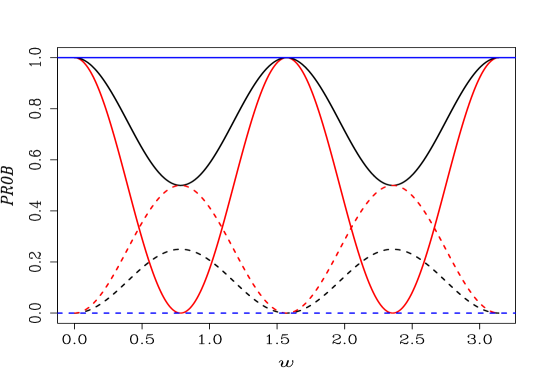
Figure 3: The same as in Fig. 2 for the case $(II)$. The continuous and dashed lines represent respectively the cases ($k_{L};-k_{L}$) and ($k_{L};k_{L}$) for distinguishable particles (black), bosons (red) and fermions (blue). The curves for ($-k_{L};-k_{L}$) are the same as for ($k_{L};k_{L}$).

Now, for distinguishable particles the probability of leaving the interaction region in different states is always larger than to do it in any of the other channels. Initially, the two bosons are in different states, but after passing through the optical grating the probability of the two particles to be in the same state reaches the $2\sin^{2}w\cos^{2}w$ value for any of the channels. The probability of finding the outgoing bosons in the same state is always larger than that for distinguishable particles. Moreover, for some values of $w$, the probability of finding the two bosons in different exit channels vanishes, giving rise to the presence of a dip. This contrasts with the behavior of distinguishable particles, for which that probability is never null. For fermions, the probability of being the two in the same channel is forbidden by Pauli’s exclusion principle (also $K=K^{\prime}$). The two fermions must always be found in different channels.

4 Multi-mode states

We move now to the more realistic case of multi-mode states. For the sake of clarity in the presentation we consider first a single particle.

4.1 Single particle

In order to have an analytically solvable model we assume both mode distributions to be Gaussian functions before the interaction with the light grating:

$$f(k,K)=g_{k_{0}}(k)G_{K_{0}}(K)={\cal N}_{g}\exp(-(k-k_{0})^{2}/\sigma^{2}){\cal N}_{G}\exp(-(K-K_{0})^{2}/\mu^{2})$$ (10)

where the normalization factors ${\cal N}_{g}$ and ${\cal N}_{G}$ are determined from the conditions $\int dk|g(k)|^{2}=1$ and $\int dK|G(K)|^{2}=1$: ${\cal N}_{g}=(2/\pi\sigma^{2})^{1/4},\cdots$. The central value of the first distribution is $k_{0}=\pm k_{L}$. We shall only consider the case $k_{0}=k_{L}$, being the extension to $k_{0}=-k_{L}$ trivial.

After the interaction we consider first the small letter variables. The Bragg scattering only takes place for modes whose momenta are very close to the Bragg angle [6]. To be concrete, the spread in velocity of particles that can be diffracted, $\sigma_{v}$, depends on the interaction time with the grating: $\sigma_{v}=1/(\tau k_{L})$. This relation can be easily derived from the time-energy uncertainty relation [10]. This property has been used to study the velocity distribution of BEC’s because the velocity selectivity of the previous condition [9]. In terms of wave vectors, this condition can be rewritten as $\sigma_{k}=m/(\tau\hbar k_{L})$. Then the modes in the interval $[k_{L}-\frac{1}{2}\sigma_{k},k_{L}+\frac{1}{2}\sigma_{k}]$ can be scattered, whereas the modes obeying $|k-k_{L}|>\sigma_{k}/2$ are always transmitted without possibility of scattering. The probability to be scattered of each mode in the interval $|k-k_{L}|\leq\sigma_{k}/2$ is given by $|c_{-}|^{2}$. Then the probability of scattering in the full beam is given by ${\cal N}_{R}|c_{-}|^{2}$, where ${\cal N}_{R}$ is the fraction of modes in the beam that can be scattered:

$${\cal N}_{R}=\int_{k_{L}-\frac{1}{2}\sigma_{k}}^{k_{L}+\frac{1}{2}\sigma_{k}}|f(k)|^{2}dk=erf\left(\frac{\sigma_{k}}{\sqrt{2}\sigma}\right)$$ (11)

with $erf$ the error function, $erf(\xi)=2\pi^{-1/2}\int_{0}^{\xi}\exp(-u^{2})du$.

On the other hand, the probability of transmission is the sum of two contributions, (a) that of the modes outside the interval $|k-k_{L}|\leq\sigma_{k}/2$, which cannot be scattered, and (b) another corresponding to the probability of modes in the interval to be transmitted without scattering, ${\cal N}_{R}|c_{+}|^{2}$. Adding both contributions we have ${\cal N}_{T}+{\cal N}_{R}|c_{+}|^{2}$, where ${\cal N}_{T}$ is the fraction of modes in the interval that cannot be scattered. Clearly, we have ${\cal N}_{T}=erfc(\sigma_{k}/(\sqrt{2}\sigma))=1-{\cal N}_{R}$.

After the interaction we have two beams, one transmitted and the other scattered, which we represent by the kets $|k_{L}>^{MM}$ and $|-k_{L}>^{MM}$. As the overlapping between these beams is negligible they can be considered orthonormal. Then although now we are in the multi-mode regime, we can use a description for the longitudinal variables with only two relevant kets because the detection process can only discriminate between the alternatives represented by these kets. If we would have used a mode-selective detection scheme the description would be inadequate. The coefficients of the kets are different from those associated with the single-mode case, containing information about the multi-mode structure ($\sigma$) and the effective window of scattering ($\sigma_{k}$). The expression $c_{+}|k_{L}>+c_{-}|-k_{L}>$ must be replaced by $d_{+}|k_{L}>^{MM}+d_{-}|-k_{L}>^{MM}$, with

$$d_{+}=e^{-i\epsilon\tau}({\cal N}_{T}+{\cal N}_{R}|c_{+}|^{2})^{1/2}\;;\;d_{-}={\cal N}_{R}^{1/2}c_{-}$$ (12)

where we have assumed that the relative phase between the reflected and transmitted components is the same that in the case of single-mode states (this is true for each mode). Clearly, we have $|d_{+}|^{2}+|d_{-}|^{2}=1$.

The relation between $\sigma$ and $\sigma_{k}$ gives the criterion for the validity of the single-mode approximation. When $\sigma\ll\sigma_{k}$, we have that $erf(\sigma_{k}/(\sqrt{2}\sigma))\rightarrow 1$ and, consequently ${\cal N}_{R}\approx 1$ and ${\cal N}_{T}\approx 0$. In this case, $d_{\pm}\approx c_{\pm}$ and it makes sense to use the single-mode approximation.

Figure 4: Scattering probability $|d_{-}|^{2}$ versus the dimensionless spread $\sigma/\sigma_{k}$ for $w=\pi/4$. The dotted line represents the single-mode scattering probability $|c_{-}|^{2}=1/2$.

Concerning the capital variables, the state can be expressed as $|K>_{G_{K_{0}}}^{MM}=\int dKG_{K_{0}}(K)|K>$. Thus, the complete state can be expressed after the interaction as

$$|f(k,K)>=|K>_{G_{K_{0}}}^{MM}(d_{+}|k_{L}>^{MM}+d_{-}|-k_{L}>^{MM})$$ (13)

From this expression it follows that the probability of detecting, for instance, a transmitted particle with transversal momentum $K$ is $|G_{K_{0}}(K)d_{+}|^{2}$. If we do not measure the perpendicular momenta, as it is usually the case, the probability of having a transmitted particle is the sum over $K$ of all these probabilities: $\int|G_{K_{0}}(K)d_{+}|^{2}dK=|d_{+}|^{2}$, because of the normalization condition. This expression shows the same form obtained in the single-mode case with the only change of $c_{\pm}\rightarrow d_{\pm}$. This change can modify the dependence on $w$, in addition to introduce the parameter $\tau$ (or the dimensionless spread $\sigma_{k}/\sigma$).

We represent $|d_{-}|^{2}$ and $|c_{-}|^{2}$ in Fig. 4. For small values of $\sigma/\sigma_{k}$ the scattering probabilities are very similar for single- and multi-mode states. In contrast, when the value of the ratio of spreads increases the multi-mode probability sharply decreases with respect to the single-mode one.

4.2 Two distinguishable particles

In the case of two incident particles the central values of $g(k)$ are equal (case $(I)$) or opposite (case $(II)$). On the other hand, for $G$ we assume both widths to be equal ($\mu$) but the mean values can be different ($G_{K_{0}}(K)$ and $G_{K_{0}^{\prime}}(K)$). The state of the two-particle system can be expressed as $|f(k,K)>_{1}|f^{\prime}(k^{\prime},K^{\prime})>_{2}$, with $f^{\prime}(k,K)=g_{k_{0}^{\prime}}(k)G_{K_{0}^{\prime}}(K)$. As in the previous example we assume that the final perpendicular momenta are not observed. Using $D_{+}=e^{-i\epsilon\tau}({\cal M}_{T}+{\cal M}_{R}|c_{+}|^{2})^{1/2}$ and $D_{-}={\cal M}_{R}^{1/2}c_{-}$ with ${\cal M}_{T}+{\cal M}_{R}=1$, for the coefficients of the second particle, we obtain

$${\cal P}_{MM}^{dis(I)}(k;k)=|d_{+}|^{2}|D_{+}|^{2}\;;\;{\cal P}_{MM}^{dis(I)}(-k;-k)=|d_{-}|^{2}|D_{-}|^{2}$$

$${\cal P}_{MM}^{dis(I)}(-k;k)=|d_{-}|^{2}|D_{+}|^{2}\;;\;{\cal P}_{MM}^{dis(I)}(k;-k)=|d_{+}|^{2}|D_{-}|^{2}$$ (14)

and

$${\cal P}_{MM}^{dis(II)}(-k;-k)=|d_{-}|^{2}|D_{+}|^{2}\;;\;{\cal P}_{MM}^{dis(II)}(k;k)=|d_{+}|^{2}|D_{-}|^{2}$$

$${\cal P}_{MM}^{dis(II)}(k;-k)=|d_{+}|^{2}|D_{+}|^{2}\;;\;{\cal P}_{MM}^{dis(II)}(-k;k)=|d_{-}|^{2}|D_{-}|^{2}$$ (15)

As $|d_{+}|^{2}+|d_{-}|^{2}=1$ and $|D_{+}|^{2}+|D_{-}|^{2}=1$ it is simple to see that all these probabilities are correctly normalized. All the probabilities are independent of the distributions $G_{K_{0}}$ as a natural consequence of not observing the final momenta. The dependence of these probabilities on $w$ clearly differs from that on the case of single mode states. For instance, ${\cal P}_{MM}^{dis(I)}(k;k)={\cal N}_{T}{\cal M}_{T}+({\cal N}_{R}{\cal M}_{T}+{\cal N}_{T}{\cal M}_{R})\cos^{2}w+{\cal N}_{R}{\cal M}_{R}\cos^{4}w$. In addition we have the dependence on $\tau$ (or $\sigma_{k}/\sigma$). We shall later represent them in Fig. 5.

4.3 Two identical particles

The final state is $N(|f(k,K)>_{1}|f^{\prime}(k^{\prime},K^{\prime})>_{2}\pm|f^{\prime}(k,K)>_{1}|f(k^{\prime},K^{\prime})>_{2})$. We have, for instance, $Nd_{+}D_{+}|k_{L}>_{1}^{MM}|k_{L}>_{2}^{MM}(|K>_{1,G_{K_{0}}}^{MM}|K^{\prime}>_{2,G_{K^{\prime}_{0}}}^{MM}\pm|K>_{1,G_{K^{\prime}_{0}}}^{MM}|K^{\prime}>_{2,G_{K_{0}}}^{MM})$ for the two particles in the channel $(k;k)$ in the case ($I$). The probability associated with the perpendicular variables has the form $2\pm 2{\cal I}$, with

$${\cal I}=Re(_{G_{K_{0}},1}^{MM}<K|K>_{1,G_{K_{0}^{\prime}}}^{MM}\;{}_{G_{K_{0}^{\prime}},2}^{MM}<K^{\prime}|K^{\prime}>_{2,G_{K_{0}}}^{MM})=$$

$$\int dK\int dK^{\prime}G_{K_{0}}(K)G_{K_{0}^{\prime}}(K^{\prime})G_{K_{0}}(K^{\prime})G_{K_{0}^{\prime}}(K)$$ (16)

The total probabilities become in the case $(I)$

$${\cal P}_{MM}^{(I)}(k;k)=2N^{2}(1\pm{\cal I})|d_{+}|^{2}|D_{+}|^{2}\;;\;{\cal P}_{MM}^{(I)}(-k;-k)=2N^{2}(1\pm{\cal I})|d_{-}|^{2}|D_{-}|^{2}$$

$${\cal P}_{MM}^{(I)}(k;-k)\equiv{\cal P}_{MM}^{(I)}(k;-k)+{\cal P}_{MM}^{(I)}(-k;k)=$$

$$2N^{2}(|d_{+}|^{2}|D_{-}|^{2}+|D_{+}|^{2}|d_{-}|^{2}\pm 2{\cal I}Re(d_{+}^{*}d_{-}D_{+}D_{-}^{*}))$$ (17)

As usual, the normalization is obtained from the condition of the sum of all the probabilities to be $1$, which reads $2N^{2}(1\pm{\cal I}(|d_{+}||D_{+}|+|d_{-}||D_{-}|)^{2})=1$.

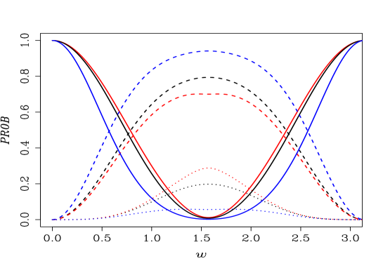
Figure 5: As Fig. 2 for multi-mode states. Bosons, fermions and distinguishable particles are represented by red, blue and black lines. We represent the case $\mu=2$, $K_{0}=1$, $K_{0}^{\prime}=2$, ${\cal N}_{T}=0.01$ and ${\cal M}_{T}=0.8$.

A specially simple situation is obtained when the two distributions $g_{k_{0}}(k)$ are equal (this condition implies $\sigma=\sigma^{\prime}$), where we have $d_{\pm}=D_{\pm}$ and the normalization condition is $N=1/\sqrt{2(1\pm{\cal I})}$. In this situation the probability distributions for bosons, fermions and distinguishable particles are equal. This result agrees with our previous discussion for single-mode states. When the initial particles are in the same state of the parallel variables the two alternatives in the expression for the state of identical particles are actually redundant and do not lead to distinctive exchange effects.

We represent the above results in figure 5. We consider the simpler case, in which ${\cal N}_{T}$ and ${\cal N}_{T}$ are constant (we must have a different spread of the multi-mode distribution for each $w$ and $\tau$). We take into account that ${\cal I}=\exp(-(K_{0}-K_{0}^{\prime})^{2}/\mu^{2})$. At variance with the single-mode case we have that the curves for bosons, and distinguishable particles (and now also for fermions) are different. Moreover, the analytical form for the case $(-k;-k)$ only shows a peak, whereas for the single-state there were two separated ones. When the values of ${\cal N}_{T}$ and ${\cal M}_{T}$ become close we recover the behavior observed for single-mode states with curves almost similar in all the cases and two peaks for $(-k;-k)$.

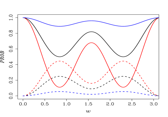
Figure 6: The same as in Fig. 3 for multi-mode states with $d_{\pm}=D_{\pm}$ and using the values $K_{0}=1$, $K_{0}^{\prime}=2$, ${\cal N}_{T}=0.1$ and $\mu=2$.

In the case $(II)$, in a similar way, we have

$${\cal P}_{MM}^{(II)}(k;-k)/2N^{2}\equiv({\cal P}_{MM}^{(II)}(k;-k)+{\cal P}_{MM}^{(II)}(-k;k))/2N^{2}=$$

$$|d_{+}|^{2}|D_{+}|^{2}+|d_{-}|^{2}|D_{-}|^{2}\pm 2{\cal I}Re(d_{+}^{*}D_{-}D_{+}^{*}d_{-})$$ (18)

$${\cal P}_{MM}^{(II)}(k;k)/2N^{2}=(1\pm{\cal I})|d_{+}|^{2}|D_{-}|^{2}\;;\;{\cal P}_{MM}^{(II)}(-k;-k)/2N^{2}=(1\pm{\cal I})|d_{-}|^{2}|D_{+}|^{2}$$

The normalization condition is given by the expression $2N^{2}(1\pm{\cal I}(|d_{+}||D_{-}|-|d_{-}||D_{+}|)^{2})=1$.

In the particular case $d_{\pm}=D_{\pm}$ ($N=1/\sqrt{2}$) the above expressions simplify to ${\cal P}_{MM}^{(II)eq}(k;-k)=|d_{+}|^{4}+|d_{-}|^{4}\mp 2{\cal I}|d_{+}|^{2}|d_{-}|^{2}$, ${\cal P}_{MM}^{(II)eq}(k;k)=(1\pm{\cal I})|d_{+}|^{2}|d_{-}|^{2}$ and ${\cal P}_{MM}^{(II)eq}(-k;-k)=(1\pm{\cal I})|d_{-}|^{2}|d_{+}|^{2}$. We represent them in Fig. 6.

The curves resemble those obtained in the single-mode case. The most important difference is that for fermions the possibility of observing simultaneously two of them in the same output arm is not null. This is due to the fact that now the perpendicular components of the momentum are different, precluding the action of the exclusion principle. It must also be noted that the visibility of the bosonic $(k;-k)$ curve is slightly reduced. In the single-mode scenario it was $1$, whereas now it does not reach that value (${\cal P}_{max,MM}^{(II)eq}(k;-k)=1$, but ${\cal P}_{min,MM}^{(II)eq}(k;-k)\neq 0$).

5 Discussion: HOM-like experiments

In this paper we have extended the theory of the two-particle Kapitza-Dirac effect to the Bragg regime. With this extension we complete the basic theory of the effect. We have derived the detection probabilities for all the possible combinations of scattering and transmission processes of the two particles. We have developed a simple model based on some reasonable assumptions to describe multi-mode states. Using this model we can quantify the differences between single- and multi-mode states. In the case of single-mode states all these probabilities can be expressed in terms of the parameter $w$, whereas for multi-mode ones one also needs to consider the duration of the interaction (or the dimensionless spread). In the single-mode case we only have exchange effects for equal perpendicular momenta, a restriction not present for multi-mode states.

We have not discussed the possibility of carrying out experimental tests of the results here derived. We refer to [7] for a brief presentation of the aspects related to the two-particle nature of the arrangement, and [6, 8] for the peculiarities associated with the Bragg regime.

Bragg’s scattering has been extensively studied for one-particle systems. In the many-particle scenario one can also find in the literature many analysis on the subject, mainly in the field of BEC (see, for instance [10]). However, there are still aspects of the problem that deserve attention. In this paper we focus on the aspects related to HOM-type experiments, which have played an important role in quantum optics, triggering a lot of activity in the field of two-photon interference experiments with beam splitters. We explore if the same relevance could be expected for massive systems, taking into account that the arrangement discussed in this paper could be used as a two-particle beam splitter.

The first point to be noted is that the coefficients $c_{+}$ and $c_{-}$ play the same role of the transmission and reflection coefficients in a beam splitter. The coefficients $c_{\pm}$ can be expressed in terms of a single parameter $w$. In the optical case the coefficients are complex variables that depend on the optical frequency. In the massive case they are also complex, but depend on the energy of the particle $e^{-i\epsilon\tau}$ and the potential strength $V_{0}$ and the duration of the interaction $\tau$ via the dimensionless parameter $w$.

Two interesting results emerge directly from our analysis. The first result concerns to particles incident on the same arm of the beam splitter. We have shown that when the particles are in single-mode states or have the same multi-mode parallel distribution there are not distinctive exchange effects and the behavior of distinguishable and identical particles becomes equal. In quantum optics we have a similar behavior. If two photons in the same state are incident in the same input arm of the beam splitter, the probabilities of finding the two photons in the different possible combinations in the output arms are the same of two classical or distinguishable particles (binomial distribution), without showing any quantum interference effect [13, 14]. Our analysis gives an intuitive explanation for the absence of distinctive exchange effects, only based on the physical meaning of the different terms of the state vector. At variance with [13, 14], we have demonstrated that exchange effects can be present in the multi-mode case, giving rise to some differences between distinguishable and identical particles. Up to our knowledge, this behavior has not been previously described in the literature. Modifying the multi-mode distributions we can modulate the differences between distinguishable and identical particles. This is an unexplored scenario where some new physical effects could emerge.

Our second result refers to the presence of dips in the case $(II)$. In quantum optics the HOM dip takes place for a perfect temporal overlapping of the two photons arriving on different arms of the beam splitter: the two photons are always found in the same output arm. In the massive case, Fig. 3 shows dips in the boson curve for some values of $w$. At these values there are not coincidence detections in the two exit paths. Thus, one of the most characteristic signatures of HOM interferometry is also present in the bosonic massive case, reinforcing the analogy between massless and massive bosons. Note a difference between the massless and massive cases. In the first one the parameters of the beam splitter (transmissivity and reflectivity) are fixed and the temporal overlapping between the photons varies. In the second one, the perfect overlapping between the two particles is assumed and one must vary $w$, the beam splitter parameter.

Finally, we shall propose a potential application of the two-particle massive beam splitter, a scheme for the verification of (anti)symmetrization. The HOM arrangement was originally conceived for precision measurements of time intervals between the arrivals of photons. Similarly, we could use our arrangement to determine if the overlapping between the wave functions of the two identical particles is large or not. If one wants to prepare identical particles in (anti)symmetrized states for some physical task, one must have some method to test that the particles are actually in that state. This can be done via double Bragg’s scattering. When the overlapping is large, the two wave functions must be (anti)symmetrized and the results derived in the previous sections for identical particles hold. In contrast, with a lower degree of overlapping the behavior of the particles becomes increasingly similar to that of distinguishable particles. These properties can be used to quantitatively measuring the degree of overlapping between the two identical particles.

Acknowledgments We acknowledge partial support from MEC (CGL 2007-60797).

References

- [1] Kapitza P L and Dirac P A M 1933 Proc. Cambridge Philos. Soc. 29 297
- [2] Gould P L, Ruff G A and Pritchard D E 1986 Phys. Rev. Lett. 56 827
- [3] Martin P J, Oldaker B G, Miklich A H and Pritchard D E 1988 Phys. Rev. Lett. 60 515
- [4] Cahn S B, Kumarakrishnan A, Shim U, Sleator T, Berman P R and Dubetsky B 1997 Phys. Rev. Lett. 79 784
- [5] Freimund D L, Aflatooni K and Batelaan H 2001 Nature 413 142
- [6] Freimund D L and Batelaan H 2002 Phys. Rev. Lett. 89 283602
- [7] Sancho P 2010 Phys. Rev. A 82 033814
- [8] Batelaan H 2000 Contemp. Phys. 41 369
- [9] Stenger J, Inouye S, Chikkatur A P, Stamper-Kurn D M, Pritchard D E and Ketterle W 1999 Phys. Rev. Lett. 82 4569
- [10] Cronin A D, Schmiedmayer J and Pritchard D E 2009 Rev. Mod. Phys. 81 1051
- [11] Hong C K, Ou Z Y and Mandel L 1987 Phys. Rev. Lett. 59 2044
- [12] Adams C S, Sigel M and Mlynek J 1994 Phys. Rep. 240 143
- [13] Loudon R 2000 The Quantum Theory of Light (Oxford Science Publications, Oxford).
- [14] Brendel J, Schütrumpf S, Lange R, Martienssen W and Scully M O 1988 Europ. Lett. 5 223 (1988); Lange R, Brendel J, Mohler E and Martienssen W 1988 ibid. 5 619