Quantum Hall effect and the different zero energy modes of graphene

Abstract

The effect of an inhomogeneous magnetic field which varies inversely as distance on the ground state energy level of graphene is studied. In this work, we analytically show that graphene under the influence of a magnetic field arising from a straight long current-carrying wire ( proportional to the magnetic field from carbon nanotubes and nanowires) exhibits zero energy solutions. We find that contrary to the case of a uniform magnetic field for which the zero energy modes show the localization of electrons entirely on just one sublattice corresponding to single valley Hamiltonian, zero energy solutions in this case reveal that the probability for the electrons to be on the both sublattices, say A and B, are the same.

Department of Science, Payame Noor University, Bijar, Iran

Young Researchers Club, Kermanshah Branch, Islamic Azad University, Kermanshah, Iran.

Keywords: Graphene; Quantun Hall effect; Zero energy modes.

1 Introduction

Graphene, a single layer of graphite, was isolated for the first time in 2004 [1]. The carbons atoms in graphene are arranged into a honeycomb structure which is consistent of the two inequivalent triangular sublattices, say A and B [2]. Electrons in graphene can hop to the nearest neighbours atoms which leads to the formation of the two energy bands, each containing the same number of states [3] and touching each other at the two inequivalent points called Dirac points, say $\textbf{K}^{+}$ and $\textbf{K}^{-}$. Around these points the energy dispersion relation of graphene is linear in momentum which implies that it s low energy excitations mimic the ultra relativistic massless particles. Thus, the low energy excitations of graphene are described by the following Dirac-like equation:

$$H=v_{F}\mbox{\boldmath$\sigma$.{p}}$$ (1)

where $v_{F}$ is the Fermi velocity and $\sigma$=$(\sigma_{x},\sigma_{y})$ is the Pauli matrices vector with $\sigma_{i}$, $i=x,y,z$, the $i$ Pauli matrix. The above equation implies that the electrons in graphene behave as massless charged Dirac fermions confined in a 2D space, an interesting feature that real particles do not exhibit because all the massless elementary particles happen to be electrically neutral. These massless electrons shows peculiar properties which massive relativistic carriers do not exhibit [4]. In fact the first experimental evidence that revealed the charged carriers in graphene mimic massless electrons was an unusual quantum Hall effect reported in 2005 [5]. In spite of this fact that charge carriers in graphene exhibit a four fold degeneracy (which comes from the real spin of electrons in addition to another factor of two, due to the equal contributions of the K-valleys, i.e. $\textbf{K}^{+}$ and $\textbf{K}^{-}$) we see that in experiments instead of quantization of the Hall conductivity in multiples of

$$\sigma_{xy}=4n\frac{e^{2}}{h}\ \ \ \ \ \ n\in\{...,-2,-1,0,1,2,...\}$$ (2)

it is observed that Hall conductivity is:

$$\sigma_{xy}=4(n+\frac{1}{2})\frac{e^{2}}{h}=4\nu\frac{e^{2}}{h},\ \ \ \ \ \ \nu=(n+\frac{1}{2}),$$ (3)

which shows that the integer quantum Hall effect (IQHE), appears in half-integers. It is also observed that unlike to the quantum Hall effect for 2D conventional systems which appears in the strong magnetic field and low temperature limit, the IQHE in graphene can be observed even at the room temperature [6]. This is because of ultra-relativistic nature of its charge carriers which mimic the massless Dirac fermions. These massless charge carriers as we’ll show later, contrary to the conventional 2D systems, show interesting results under the influence of a uniform magnetic field. We, before discussing the effect of a constant magnetic field $\textbf{B}=B_{z}$ perpendicular to the graphene’s plane, note that even for conventional 2D systems, the periodic potential due to the host lattice is of no relevance to the quantum Hall problem because the size of the electron wave packet in a magnetic field is much larger than the lattice period. The periodic potential due to the lattice is, therefore, neglected in studies of the quantum Hall effect, however if one considers to calculate the Landau levels based on the tight-binding model, the commensurability problem between the magnetic flux and lattice unit cell is needed to be considered. This problem is known to inevitably occur in the two dimensional electron system [7-9]. However, interestingly for graphene the periodic potential of the honeycomb lattice is already built-in and therefore it is counted in the massless Dirac-like equation. Thus, we do not really need to incorporate explicitly the periodic potential term into the Dirac equation.
Now, in order to obtain the energy spectrum of graphene in the presence of a uniform magnetic field which is considered to be perpendicular to the garphene’s plane, by choosing the symmetric gauge and taking the units such that $c=1$, the single valley Hamiltonian of graphene can be written as:

$$H=v_{F}\left(\begin{array}[]{cc}0&\Pi_{x}-i\Pi_{y}\\ \Pi_{x}+i\Pi_{y}&0\\ \end{array}\right),$$ (4)

where

$$\mbox{\boldmath$\Pi$}=-i\hbar(\partial_{x}-\frac{iy}{2l^{2}},\partial_{y}+\frac{ix}{2l^{2}}),\ \ \ \ \ l^{2}=\frac{\hbar}{B|e|}$$ (5)

Then, one may write the equation (4) in the form of the following eigenvalue equation:

$$(i\hbar\partial_{t}+i\hbar v_{F}\sigma_{x}\Pi_{x}+i\hbar v_{F}\sigma_{y}\Pi_{y})\Psi_{\textbf{K}^{+}}(\textbf{r},t)=0.$$ (6)

Next, multiplying the above equation by $\sigma_{z}$ (the z-component of Pauli matrix) gives:

$$(i\hbar\hat{\gamma}^{0}\partial_{t}+i\hbar v_{F}\hat{\gamma}^{1}\Pi_{x}+i\hbar v_{F}\hat{\gamma}^{2}\Pi_{y})\Psi_{\textbf{K}^{+}}(\textbf{r},t)=0,$$ (7)

with the $\hat{\gamma}$ matrices as:

$$\hat{\gamma}^{0}=\left(\begin{array}[]{cc}1&0\\ 0&-1\end{array}\right)\ ,\ \hat{\gamma}^{1}=\left(\begin{array}[]{cc}0&1\\ -1&0\end{array}\right)\ ,\ \hat{\gamma}^{2}=\left(\begin{array}[]{cc}0&-i\\ -i&0\end{array}\right).$$ (8)

Here in order to solve the equation (7), we split the 2-spinor $\Psi_{\textbf{K}^{+}}$ into its sublattice parts:

$$\Psi_{\textbf{K}^{+}}(\textbf{r},t)=\left(\begin{array}[]{c}\varphi\\ \psi\end{array}\right)e^{i\frac{E}{\hbar}t},$$ (9)

which inserting it into the equation (7) leads us to the following expression:

$$\left(\begin{array}[]{c}\ \ \dot{\varphi}\\ -\dot{\psi}\end{array}\right)=\left(\begin{array}[]{cc}0&S\\ D&0\end{array}\right)\left(\begin{array}[]{c}\varphi\\ \psi\end{array}\right),$$ (10)

where $S$ and $D$ are given by:

$$S=-v_{F}(\partial_{x}-\frac{iy}{2l^{2}})+iv_{F}(\partial_{y}+\frac{ix}{2l^{2}}),$$ (11)

$$D=v_{F}(\partial_{x}-\frac{iy}{2l^{2}})+iv_{F}(\partial_{y}+\frac{ix}{2l^{2}}).$$ (12)

There is no need to say that from equation (10) one can obtain the following second order differential equations:

$$\ddot{\varphi}=-SD\varphi,$$ (13)

$$\ddot{\psi}=-DS\psi,$$ (14)

which by introducing the following dimensionless quantities:

$$x\rightarrow\widetilde{x}=\frac{x}{l},\ \ \ \ \ y\rightarrow\widetilde{y}=\frac{y}{l},$$ (15)

we can solve the them with respect to $\varphi$ and $\psi$. In order to do so, we first need to make the following ansatz:

$$\varphi(\textbf{r},t)=e^{-iEt/\hbar}\varphi(\textbf{r}),$$ (16)

and

$$\psi(\textbf{r},t)=e^{-iEt/\hbar}\psi(\textbf{r}),$$ (17)

which plugging them in the equations (13) and (14) yields:

$$E^{2}=\frac{\hbar^{2}v_{F}^{2}}{l^{2}}\left[(-i\partial_{\widetilde{x}}-\frac{\widetilde{y}}{2})^{2}+(-i\partial_{\widetilde{y}}+\frac{\widetilde{x}}{2})^{2}\pm\frac{1}{l^{2}}\right].$$ (18)

where the positive (minus) sign corresponds to the solution for $\varphi$ ($\psi$). Transforming to the complex coordinates:

$$z=\widetilde{x}-i\widetilde{y},\ \ \ \bar{z}=\widetilde{x}+i\widetilde{y},$$ (19)

gives the equation (18) as follows:

$$E^{2}=\frac{\hbar^{2}v_{F}^{2}}{l^{2}}\left[-4\partial_{z}\partial_{\overline{z}}+\frac{1}{4}z\overline{z}+\overline{z}\partial_{\overline{z}}-z\partial_{z}\pm 1\right]$$ (20)

At this point, we can define the ladder operators $\hat{a}^{{\dagger}}$ and $\hat{a}$ as:

$$\hat{a}^{{\dagger}}=\frac{1}{\sqrt{2}}(\frac{\bar{z}}{2}-2\partial_{z}),\ \ \ \hat{a}=\frac{1}{\sqrt{2}}(\frac{z}{2}+2\partial_{\bar{z}}),$$ (21)

which from them, one can write the solution for $\varphi$ in the following form:

$$E^{2}=\frac{2\hbar^{2}v_{F}^{2}}{l^{2}}\left[\hat{a}^{{\dagger}}\hat{a}+1\right],$$ (22)

where $\hat{N}=\hat{a}^{{\dagger}}\hat{a}$, with the eigenvalues n=0,1,…, is the number operator. While for $\psi$, we obtain the following solution:

$$E^{2}=\frac{2\hbar^{2}v_{F}^{2}}{l^{2}}\hat{a}^{{\dagger}}\hat{a}.$$ (23)

Here, the two solutions could be packed in one equation as:

$$E^{2}=\frac{\hbar^{2}v_{F}^{2}}{l^{2}}\left[2(n+\frac{1}{2})\pm 1\right]$$ (24)

At this point one can express the square of the Hamiltonian (4) in terms of the number operator $\hat{N}$:

$$H^{2}=\frac{2\hbar^{2}v_{F}^{2}}{l^{2}}\left(\begin{array}[]{cc}\hat{N}+1&0\\ 0&\hat{N}\\ \end{array}\right),$$ (25)

with the following eigenstates and eigenvalues for $H$:

$$\Psi_{n,\textbf{K}^{+}}=\frac{1}{\sqrt{2}}\left(\begin{array}[]{c}|n-1\rangle\\ \pm|n\rangle\\ \end{array}\right),\ \ \ \ E_{n}=\pm\frac{\hbar v_{F}}{l}\sqrt{2n}$$ (26)

It is clear that for $n\neq 0$ we have one pairs of eigenstates and eigenvalues but for $n=0$ (corresponding to $E=0$) we have:

$$\Psi_{0,\textbf{K}^{+}}=\left(\begin{array}[]{c}0\\ |0\rangle\\ \end{array}\right)$$ (27)

It is clear that the solution corresponding to the $\textbf{K}^{+}$ ($\textbf{K}^{-}$) point shows that the probability for the electrons to be on the sublattice A (B) is zero. Thus, the zero solution corresponding to $\textbf{K}^{+}$ ($\textbf{K}^{-}$) implies the localization of Dirac fermions on the B (A) sublattice. In the original experimental paper it is argued that since in all the $n\neq 0$ energy levels both pseudospin states are filled, whereas in the $n=0$ level only one is, the density of states in the latter case is 1/2 that of the other levels and therefore it contributes only $\frac{e^{2}}{2h}$ per spin/valley.
The above argument does not seem entirely satisfactory, since, as it is clear from general solutions (26), any given eigenstate is normalized to one irrespective of whether one pseudospin component is zero or not. Hence the half contribution ($\frac{e^{2}}{2h}$ ) of the zero energy mode corresponding to the single valley index could not be explained in this way because, as we see from the normalized eigenstates, electrons localize on just one sublattice, instead of being contributed half on the sublattice A and half on the sublattice B.
There are another explanation for observation of half-integer quantum Hall effect that says since for $n=0$ we have only one solution (as there is no difference between $+|0\rangle$ and $-|0\rangle$) the degeneracy of this level is half of the other energy levels for which there exist two solutions. What is wrong about this conclusion is that existence of just one solution for $n=0$ level (and two for others), does not simply mean that its degeneracy is twice smaller because one of the two solutions corresponds to the negative energy states (holes) and another to the positive energy states (electrons). Therefore this assumption could be disregarded.
Another explanation might be based on this assumption that the level $n=0$ is equally shared by electrons and holes, meaning that it is half filled with electrons and half with the holes, since there is no difference between $+|0\rangle$ and $-|0\rangle$ in this level [10]. In the other words the ground state energy level is completely filled with the same types of fermions except the fact that they only differ by their charge which does not prevent them from being subject to the Pauli exclusion principle. It is by now that one can say the $n=0$ energy level contributes $1/2(e^{2}/h)$. Hence, as for the other levels two kind of fermions (holes and electrons) with the same number of states contribute in the conductance, they contribute twice of $1/2(e^{2}/h)$ per spin/valley.
The interesting feature that zero energy solutions exhibit, motivate us to seek zero energy modes by examining the effect of other types of magnetic fields on graphene’s energy spectrum. In fact, when the strength of the magnetic field is high the ground state energy level is occupied by more and more electrons because the degeneracy of the levels increase and therefore the lowest levels play significant role in this case. In this paper, we examine the effect of an inhomogeneous magnetic field which varies as $B=(0,0,1/x)$ on the lowest energy level and show that it exhibits zero energy solutions which is different from those obtained for the case of the constant magnetic field discussed above. As it is well-known, this magnetic field occurs around a straight long current-carrying wire (see Fig. 1). We first, in the next section briefly discuss the supersymmetric quantum mechanics and the shape invariant method [11-14] which turns out to be useful for our investigation.

2 Supersymmetric quantum mechanics

One of the methods for solving the quantum mechanical problems is based on finding the relation between ground state wave function and the corresponding potential. Considering the Hamiltonian $H(x)$ as:

$$H(x)=-\frac{d^{2}}{dx^{2}}+V(x),$$ (28)

with associated eigenfunctions and eigenvalues $\psi_{n}(x)$ and $E_{n}$, respectively, we can write:

$$H(x)\psi_{n}(x)=E_{n}\psi_{n}(x)$$ (29)

Now, if one defines $H_{1}(x)$ as:

$$H_{1}(x)\psi_{n}(x)=H(x)-E_{0},$$ (30)

so that its ground state energy become zero ($E_{0}$ is the ground state energy of $H(x)$), we can write:

$$H_{1}(x)=-\frac{d^{2}}{dx^{2}}+V_{1}(x)=-\frac{d^{2}}{dx^{2}}+V(x)-E_{0},$$ (31)

It is clear that the two Hamiltonians $H(x)$ and $H_{1}(x)$ have the same eigenfunctions. Denoting the eigenfunctions and eigenvalues of $H_{1}(x)$ with $\psi_{n}^{1}(x)$ and $E^{1}_{n}$, respectively, we can write:

$$H_{1}(x)\psi_{n}(x)=(E_{n}-E_{0})\psi_{n}(x)\ \ \rightarrow\ \ \psi_{n}(x)=\psi_{n}^{1}(x),\ \ \ E^{1}_{n}=E_{n}-E_{0}$$ (32)

Now with defining the ladder operators $\hat{A}$ and $\hat{A}^{{\dagger}}$ as:

$$\hat{A}=\frac{d}{dx}+W(x),\ \ \ \ \ \hat{A}^{{\dagger}}=-\frac{d}{dx}+W(x),$$ (33)

where $W(x)$ is called superpotential, one can write $H_{1}(x)$ in terms of the above operators as:

$$H_{1}(x)=\hat{A}^{{\dagger}}\hat{A}=-\frac{d^{2}}{dx^{2}}+V_{1}(x),$$ (34)

Here we see that from the relations (31) and (33) one can arrive at the following relation for $V_{1}(x)$:

$$V_{1}(x)=W^{2}(x)-\frac{dW(x)}{dx}$$ (35)

and keeping in mind that the ground state energy of $H_{1}(x)$ is zero, we arrive at:

$$H_{1}(x)\psi_{0}^{1}(x)=\hat{A}^{{\dagger}}\hat{A}\psi_{0}^{1}(x)=0,$$ (36)

which means that $\hat{A}$ annihilates the ground state wave function $\psi_{0}^{1}(x)$, i.e.:

$$\hat{A}\psi_{0}^{1}(x)=0$$ (37)

Now it is obvious that from equations 34-36 one can write the ground state wave function with respect to the superpotential $W(x)$ and vise versa:

$$\psi_{0}(x)=Ne^{-\int^{x}W(x)dx}\ \ \leftrightarrow\ \ W(x)=-\frac{d}{dx}\ln\psi_{0}(x)=-\frac{1}{\psi_{0}(x)}\frac{d\psi_{0}(x)}{dx}$$ (38)

It is by now that we can define Hamiltonian $H_{2}(x)$, partner of $H_{1}(x)$, which we denote them with $H_{+}(x)$ and $H_{-}(x)$ from now on, respectively, as follows:

$$H_{+}(x)=\hat{A}\hat{A}^{{\dagger}}=-\frac{d^{2}}{dx^{2}}+V_{+}(x),$$ (39)

with

$$V_{+}(x)=W^{2}(x,a_{0})+\frac{dW(x,a_{0})}{dx}$$ (40)

The supersymmetric partner potential $V_{-}$ and $V_{+}$ are supposed to be shape invariant if they satisfy the following equation:

$$V_{+}(x,a_{0})=V_{-}(x,a_{1})+R(a_{0}),$$ (41)

which means that two supersymmetric partner potentials have the same form, but are characterized by the different values of parameters $a_{0}$ and $a_{1}$ . To be more specific, the parameter $a_{1}$ is a function of $a_{0}$, namely, $a_{1}$ = R($a_{0}$) with R an independent function of $x$. Now one can obtain the energy spectrum associated to $V_{-}(x,a_{0})$ simply from the shape invariance condition as:

$$E_{n}^{-}(a_{0})=\sum_{i=0}^{n-1}R(a_{i}),$$ (42)

where for $n>0$:

$$E_{0}^{-}(a_{0})=0$$ (43)

while the corresponding wave functions are given by:

$$\psi^{-}_{n}(x,a_{0}) \sim\hat{A}^{{\dagger}}(x,a_{0})\hat{A}^{{\dagger}}(x,a_{1})...\hat{A}^{{\dagger}}(x,a_{0})(x,a_{1})\psi^{-}_{0}(x,a_{n})$$

$$=\hat{A}^{{\dagger}}(x,a_{0})\psi^{-}_{n-1}(x,a_{1}).$$ (44)

Note that there are only a few problems that satisfy the shape invariant condition (41). As we show in the next section, although the ground state energy level can be obtained analytically, the shape invariant condition is not satisfied.

3 Zero energy modes corresponding to effect of a varying magnetic field

As we’ll show in what follows, graphene spectrum under the influence of a magnetic field which varies as inverse of distance, i.e. $\textbf{B}=(0,0,1/x)$ exhibits zero energy modes. This magnetic field occurs often, as it is the magnetic filed around a long, straight current-carrying wire. In fact because of the symmetry of the wire the magnetic lines are circles concentric with it and lie in the planes perpendicular to the wire. The magnetic field B is constant on any circle of radius $R$ and is given by:

$$\textbf{B}=\frac{\mu_{0}I}{2\pi R}$$ (45)

where $I$ is the current of the wire and $\mu_{0}$ is the magnetic constant. Now if we consider a graphene sheet which lies parallel to the axis of wire so that the lines of the magnetic field intersect the graphene sheet which is assumed to be in xy-plane, the corresponding vector potential can be written as:

$$\textbf{A}=(0,q\ln x,0),\ \ \rightarrow\textbf{B}=(0,0,q\frac{1}{x}),$$ (46)

where we have used the Landau gauge and defined q to be:

$$q=\frac{\mu_{0}I}{2\pi}.$$ (47)

At this point, if we go through the same procedure as the case of the constant magnetic field (see section 1), in this case, we’ll obtain for the $S$ and $D$ (with taking $v_{F}=1$ in our evaluations):

$$S =-\partial_{x}+i(\partial_{y}-iqe\ln x),$$

$$D =\partial_{x}+i(\partial_{y}-iqe\ln x).$$ (48)

In the next step by taking the units such that $\hbar=c=1$, we can make the following ansatz:

$$\Psi(\textbf{r},t)=\left(\begin{array}[]{c}\varphi\\ \psi\\ \end{array}\right)e^{iEt},$$ (49)

which leads us to the following equation:

$$E^{2}\psi(\textbf{r})=\left\{-\mbox{\boldmath$\nabla$}^{2}+q^{2}e^{2}\ln^{2}x+2iqe\ln x\partial_{y}+\frac{qe}{x}\right\}\psi(\textbf{r}).$$ (50)

We then make the following ansatz for $\psi(\textbf{r})$ as:

$$\psi(\textbf{r})=e^{ik_{y}y}f(x),$$ (51)

which plugging it into (50) gives:

$$\left[-\frac{d^{2}}{dx^{2}}+k^{2}_{y}+q^{2}e^{2}\ln^{2}x-2qek_{y}\ln x+\frac{qe}{x}\right]f(x)=E^{2}f(x)$$ (52)

The above equation is an eigenvalue equation that can be written as:

$$H(x)f(x)=\epsilon f(x),\ \ \ \ \epsilon=E^{2}$$ (53)

It is by now that we can write the superpotential $W(x)$ in the form:

$$W(x)=-a\ln x+\frac{b}{a}.$$ (54)

Then we define Hamiltonian $H_{1}(x)$ as:

$$H_{1}(x)=-\frac{d^{2}}{dx^{2}}+V_{1}(x)=-\frac{d^{2}}{dx^{2}}+V(x)-\epsilon_{0},$$ (55)

where $\epsilon_{0}$ is the ground state energy of $H(x)$ and $V_{1}(x)$ by the use of the relation:

$$V_{1}(x)=W^{2}(x)-\frac{dW(x)}{dx},$$ (56)

is given by:

$$V_{1}(x)=a^{2}\ln^{2}x-2b\ln x+\frac{a}{x}+\frac{b^{2}}{a^{2}}.$$ (57)

Now by comparing the two Hamiltonians $H(x)$ and $H_{1}(x)$, one can get $a$ and $b$ as:

$$a=qe,\ \ \ b=qek_{y},$$ (58)

which reveals that they are just the same and, therefore, we obtain:

$$\epsilon_{0}=0,$$ (59)

meaning that the ground state energy level, $E_{0}$, is zero. Here we should note that the other energy levels can not be derived analytically because the shape invariant condition (41) is not satisfied. We also note that for $\varphi(r)$ the same result is obtained, since we the commutation relation:

$$[S,D]=0,$$ (60)

is satisfied, meaning that the $x$ and $y$ components of dynamical momentum do not commute with each other. Thus, we have arrived at a very important result. For graphene under a varying magnetic field discussed above, there exists two zero energy modes for which the probability for Dirac fermions to be on the sublattice $A$ is the same as sublattice $B$. However this does not mean that these zero energy are different to those obtained for uniform magnetic field in the sense of living electrons on the two sublattices. It is because, as we pointed out in the first section, the wave function for the other Dirac point are swapped for a constant magnetic field and therefore in an uniform magnetic field electrons are present on both triangular sublattices as well as the electrons in a varying magnetic field. The whole argue is about the single valley Hamiltonian which One can also obtained $f_{0}(x)$ as follows:

$$f_{0}(x)=N\exp(eqx\ln x-eqx-k_{y}x)$$ (61)

where $N$ is the normalization constant and subscribe $0$ shows that $f_{0}(x)$ is the wave function associated to the lowest energy level. Note that, here $x$ takes its positive values ($x>0$). It may be assumed that the existence of the two Dirac points has completely fixed the zero of the energy at these points, however, interestingly, for a magnetic field which varies inversely as square of distance, i.e. B=($0,0,\lambda/x^{2}$) (where $\lambda$ is a constant), the energy spectrum can be obtained analytically using the shape invariant method as [15]:

$$E_{n}=\pm v_{F}\sqrt{k_{y}^{2}-\frac{\lambda^{2}e^{2}k_{y}^{2}}{(n+1/2+\sqrt{1/4+\lambda e(\lambda e-1)})^{2}}},$$ (62)

which shows that for $k_{y}\neq 0$, the $n=0$ energy level ($E_{0}$) is not zero, unlike the ground state energy due to the effect of the magnetic field from a long current-carrying wire which revealed (even for nonzero values for $k_{y}$ ) to be zero.

4 Implications for experiment

No zero energy modes are observed when a magnetic field is applied to a system consistent of electrons confined in a conventional two dimensional structure, since charge carriers in conventional 2D systems obey the schrödinger equation of motion and therefore no massless carriers are imagined for them. However, it does not mean that strong magnetic field can not be applied to these systems which give rise to the observation of conventional quantum Hall effect. The problem is about the magnetic field discussed in the previous section. In fact, one arrives at no analytical solution when the effect of the magnetic field $\textbf{B}=(0,0,q/x)$ (see Eq. (46)) is examined on the massive carries no mater whether they behave relativistically or not. This may be the reason why no investigations has been reported up to now concerning the effect that this kind of magnetic field might have on conventional 2D system.
From the above discution we see that graphene could be considered as the only 2D structure that investigation regarding the effect of the magnetic field (46) - both from the theoretical and experimental point of view - is worth noting. As it is shown in Fig.1, the magnetic lines lie in the planes perpendicular to the wire and intersect the graphene’s plane. The magnetic field B which is constant on any circle of radius R, decrease inversely as the distance increases in the $x$-direction.
Here, there is no need to say that the result reported in this paper regarding the existence of zero energy modes could be put to the test in contrast with other types of nonuniform magnetic fields such as that varies inversely as square of the distance $x$ (see equation 62) and those investigated in [16].

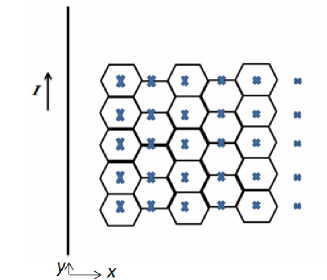
Figure 1: Left: The lines of the magnetic field from a current carrying wire which in the xy-plane decreases as $1/x$, lie in the planes perpendicular to the wire and intersect the graphene’s sheet. Right: The density distribution associated with the $f_{0}(x)$ for currents $I_{1}$ (green line) and $I_{2}$ (red line) for which $I_{2}=2I_{2}$ . As it is expected the width of the wave-packet grows as the current I -and therefore the magnetic field- decreases.

In the end of this section, we should note that the magnetic field created by a toroid for a special case varies inversely as distance as well. However, it is often used to create an almost uniform magnetic field in some enclosed area. One can use Ampere s law to obtain the magnetic field inside of a toroid with N turns of wire as:

$$B=\frac{\mu NI}{2\pi r}$$ (63)

where r which is measured from the center of the toroid is the radius of a circle to which the direction of the magnetic field is tangent. In fact the magnetic filed is approximately uniform inside the torus, if the radius of toroid, r, is very large compared with the cross-sectional radius of it. But for small values of r the magnetic field falls off inversely as r. So our results can also hold for this case as well.

5 Conclusion

In this work, we examined the effect of a magnetic field varying inversely as distance on the ground state energy level of graphene. One important reason for studying this type of magnetic field- apart from this fact that it occurs often-is that it is . In fact it is the magnetic field of a long carrying-current wire and, therefore, it can be important when it comes to applications of carbon nanotubes and nanowires with graphene. We also showed that graphene under the influence of such a magnetic field exhibits zero energy modes which is kind of different from the zero energy modes corresponding to the uniform magnetic filed (counted for the observation of the unconventional quantum Hall effect in graphene). In fact, contrary to the former case, the zero energy solutions associated to the magnetic field $B=(0,0,q\frac{1}{x})$ do not show the localization of Dirac fermions on just one sublattice but they imply that the probability to find electrons on one sublattice, say A, is the same as other one, say B. We also discussed the original interpretation of observation of the half-integer quantum Hall effect in graphene which does not seem to be complectly satisfactory because the localization of electrons on one sublattice does not imply that the density of states due to the $n=0$ Landau level is half of the others. We also discussed about how the effect of the two kind of magnetic field which varied as $1/x^{2}$ and $1/x$ on the graphene spectrum could lead to the different results.
In this work we investigated the effect of a the latter case on the massless Dirac fermions of undoped graphene, leading to observation of two zero energy modes which, as we said, are different in the sense of living the electrons on the different sublattices (per valley/spin). As we pointed out, considering the massive relativistic particles no analytical solution for the lowest energy level is obtained and it might be the reason that the potential (45) have not been considered up to now.
In the end, we should note that at the first sight it might seem strange that the localization of charge carriers differs for the varying and constant magnetic field. However, by considering the two Dirac points we see that one indicates the localization of electrons on B and another on the A sublattice and therefore the equivalency of carbon atoms is not broken.
Another point which is worth noting here is that the magnetic energy levels obtained from the tight-binding model agrees well with that calculated from the kp model [17].

References

- [1] K.S. Novoselov et al., Sience 306, 666 (2004)
- [2] A. Castro-Neto et al., Rev. Mod. Phys. 81, 109 (2009).
- [3] Wallace, P. R. Phys. Rev. 71, 622 (1947)
- [4] M.R Setare and D. Jahani, J. Phys.: Condens. Matter 22, 245503(2010).
- [5] Y. B. Zhang, Y. W. Tan, H. L. Stormer, and P. Kim, Nature, 438, 201 (2005).
- [6] K. S. Novoselov et al., Science, 315, 1379 (2007)
- [7] D. R. Hosfstadter, Energy levels and wave functions of Bloch electrons in rational and irrational magnetic fields, Phys. Rev. B 14, 2239 (1976).
- [8] R. Rammal, J. Phys.46, 1345 (1985).
- [9] K. Wakabayashi, M. Fujita, H. Ajiki, and M. Sigrist, Phys. Rev. B 59, 8271-8282 (1999).
- [10] V.P. Gusynin and S.G. Sharapov, Phys. Rev B 73, 245411 (2006).
- [11] E. Witten, Nucl. Phys. B 188, 513 (1981).
- [12] F. Cooper, B. Freeman, Ann. Phys. 146, 262 (1983).
- [13] L. Gendenshtein, JETP Lett. 38, 356 (1983).
- [14] F. Cooper, A. Khare and U. Sukhatme, Supersymmetry in Quantum Mechanics (Singapore: World Scientific), (2001).
- [15] M. R. Setare, D. Jahani, Int. J. Mod. Phys B. 25, 365, (2001)
- [16] Ş. Kuru et al, J. Phys.: Condens. Matter 21, 455305 (2009).
- [17] Z. Z. Zhang, Kai Chang, F. M. Peeters, Phys. Rev. B 77, 235411 (2008).