3D Terrestrial lidar data classification of complex natural scenes using a multi-scale dimensionality criterion: applications in geomorphology.

Abstract

3D point clouds of natural environments relevant to problems in geomorphology (rivers, coastal environments, cliffs,…) often require classification of the data into elementary relevant classes. A typical example is the separation of riparian vegetation from ground in fluvial environments, the distinction between fresh surfaces and rockfall in cliff environments, or more generally the classification of surfaces according to their morphology (e.g. the presence of bedforms or by grain size). Natural surfaces are heterogeneous and their distinctive properties are seldom defined at a unique scale, prompting the use of multi-scale criteria to achieve a high degree of classification success. We have thus defined a multi-scale measure of the point cloud dimensionality around each point. The dimensionality characterizes the local 3D organization of the point cloud within spheres centered on the measured points and varies from being 1D (points set along a line), 2D (points forming a plane) to the full 3D volume. By varying the diameter of the sphere, we can thus monitor how the local cloud geometry behaves across scales. We present the technique and illustrate its efficiency in separating riparian vegetation from ground and classifying a mountain stream as vegetation, rock, gravel or water surface. In these two cases, separating the vegetation from ground or other classes achieve accuracy larger than 98 %. Comparison with a single scale approach shows the superiority of the multi-scale analysis in enhancing class separability and spatial resolution of the classification. Scenes between ten and one hundred million points can be classified on a common laptop in a reasonable time. The technique is robust to missing data, shadow zones and changes in point density within the scene. The classification is fast and accurate and can account for some degree of intra-class morphological variability such as different vegetation types. A probabilistic confidence in the classification result is given at each point, allowing the user to remove the points for which the classification is uncertain. The process can be both fully automated (minimal user input once, all scenes treated in large computation batches), but also fully customized by the user including a graphical definition of the classifiers if so desired. Working classifiers can be exchanged between users independently of the instrument used to acquire the data avoiding the need to go through full training of the classifier. Although developed for fully 3D data, the method can be readily applied to 2.5D airborne lidar data.

1 Introduction

Terrestrial laser scanning (TLS) is now frequently used in earth sciences studies to achieve greater precision and completeness in surveying natural environments than what was feasible a few years ago. Having an almost complete and precise documentation of natural surfaces has opened up several new scientific applications. These include the detailed analysis of geometric properties of natural surfaces over a wide range of scales (from a few cm to km), such as 3D stratigraphic reconstruction and outcrop analysis [22, 35], grain size distribution in rivers [17, 16, 15], dune fields[31, 30], vegetation hydraulic roughness [5, 4], channel bed dynamics [29] and in situ monitoring of cliff erosion and rockfall characteristics [1, 26, 34, 36, 43].For all these applications, precise automated classification procedures that can pre-process complex 3D point cloud in a variety of natural environments are highly desirable. Typical examples of applications are the separation of vegetation from ground or cliff outcrops, the distinction between fresh rock surfaces and rockfall, the classification of flat or rippled bed and more generally the classification of surfaces according to their morphology. Yet, developing such procedures in the context of geomorphologic applications remains difficult for four reasons : (1) the 3D nature of the data as opposed to the traditional 2D structures of digital elevation models (DEM), (2) the variable degree of resolution and completeness of the data due to inevitable shadowing effects, (3) the natural heterogeneity and complexity of natural surfaces, and (4) the large amount of data that is now generated by modern TLS. In the following we describe these difficulties and how efficient 3D classification is critically needed to advance our use of TLS data in natural environments.

1. Terrestrial lidar data are mostly 3D as opposed to digital elevation models or airborne lidar data which can be considered 2.5D. This means that traditional data analysis methods based on raster formats (in particular the separation of vegetation from ground, e.g. [42]) or 2D vector data processing cannot in general be applied to ground based lidar data. In some cases, the studied area in the 3D point cloud is mostly 2D at the scale of interest (i.e., river bed [17], cliff [36, 2], estuaries [13]) and can be projected and gridded to use existing fast raster based methods. However in many cases the natural surface is 3D and there is no simple way to turn it into a 2D surface (e.g., Fig. 1). In other cases rasterizing a large scale 2D surface becomes non-trivial when sub-pixel features (vegetation, gravel, fractures…) are significantly 3D. In a river bed for instance, this amounts at locally classifying the data in terms of bed surface and over-bed features (typically vegetation) which requires a 3D classification approach.

Figure 1: Left : Steep mountain river bed in the Otira gorge (New-Zealand), and Terrestrial Laser Scanner location. Right: part of the point cloud rendered using PCV technique in CloudCompare [12] showing the full 3D nature of the scene (3 millions points, minimum point spacing = 1 cm). Identifying key elementary classes such as vegetation, rock surfaces, gravels or water surfaces would allow to study the vertical distribution of vegetation, the water surface profile, to segment large boulders, or to measure changes in gravel cover and thickness between surveys.

2. Terrestrial lidar datasets are all prone to a variable degree to shadow effects and missing data (water surface for instance) inherent to the ground based location of the sensor and the roughness characteristics of natural surfaces (e.g. 1). While multiple scanning positions can significantly reduce this issue, it is sometimes not feasible in the field due to limited access or time. Interpolation can be used to fill in missing information (e.g., meshing the surface), but it is quite complicated in 3D, and can lead to spurious results owing to the high geometrical complexity of natural surfaces. Arguably, interpolation should be used as a last resort, and in particular only after the 3D scene has been correctly classified to remove, for instance, vegetation. Hence, any method to classify 3D point clouds should account for shadow effects, either by being insensitive to it, or by factoring in that data are locally missing.

3. As shown in a scan of a steep mountain stream, natural surfaces can exhibit complex geometries (fig. 1). This complexity arises from the non-uniformity of individual objects (variable grain size, type and age of vegetation, variable lithology and fracture density …), the large range of characteristic spatial scales (from sand to boulders, grass to trees) or its absence (fractures for instance). This makes the classification of raw 3D point cloud data arguably more complex than artificial structures such as roads or buildings which have simpler geometrical characteristics (e.g., plane surface or sharp angles)

4. As technology evolves, data sets are denser and larger which means that projects with billions of points are likely to become common in the next decade. Automatic processing is thus urgently needed, together with fast and precise methods minimizing user input for rapidly classifying large 3D points clouds.

To our knowledge no technique has been proposed to classify natural 3D scenes as complex as the one in fig. 1 into elementary categories such as vegetation, rock surface, gravels and water. Classification of simpler environments into flat surfaces and vegetation has been studied for ground robot navigation [45, 23] using purely geometrical methods, but was limited by the difficulty in choosing a specific spatial scale at which natural geometrical features must be analyzed. Classification based on the reflected laser intensity has recently been proposed [11], but owing to the difficulty in correcting precisely for distance and incidence effects (e.g. [19, 24]), it cannot yet be applied to 3D surfaces. Classification based on RGB imagery can be used in simple configurations to separate vegetation from ground for instance [24]. But for large complex 3D environment, the classification efficiency is limited by strong shadow projections (fig. 1), image exposure variations, effects of surface humidity as well as the limited separability of spectral signature of RGB components [24]. Moreover, when the objective is to classify objects of similar RGB characteristics but different geometrical characteristics (i.e. flat bed vs ripples, fresh bedrock vs rockfall), only geometry can be used to separate points belonging to each class.

In this paper, we present a new classification method for 3D point clouds specifically tailored for complex natural environments. It overcomes most of the difficulties discussed above: it is truly 3D, works directly on point clouds, is largely insensitive to shadow effects or changes in point density, and most importantly it allows some degree of variability and heterogeneity in the class characteristics. The set of softwares designed for this task (the CANUPO suite) is coded to handle large point cloud datasets. This tool can be used simply by non-specialists of machine learning both in an automated way and also by allowing an easy control of the classification process. Because geometrical measurements are independent of the instrument used (which is not the case for reflected intensity [19]or RGB data), classifiers defined in a given setting (i.e. mountain rivers, salt marsh environment, gravel bed river, cliff outcrop…) can be directly reused by other users and with different instruments without a mandatory phase of classifier reconstruction.

The strength of our method is to propose a reliable classification of the scene elements based uniquely on their 3D geometrical properties across multiple scales. This allows for example recognition of the vegetation on complex scenes with very high accuracy (i.e. $\approx 99.6\%$ in a context such as fig. 1). We first present the study sites and data acquisition procedure. We then introduce the new multi-scale dimensionality feature that is used to describe the local geometry of a point in the scene and how it can characterizes simple elementary environment features (ground and vegetation). In section 4, we describe the training approach to construct a classifier: it aims at automatically finding the combination of scales that best allows the distinction between two or more features. The quality of the classification method is tested on two data sets: a simple case of riparian vegetation above sand, and a more complex, multiple class case of a mountain river with very pronounced heterogeneity and 3D features (fig. 1). Finally, we discuss the limitation and range of application of this method with respect to other classification methods.

2 Study sites and data acquisition

The method is tested on two different environments : a pioneer salt marsh environment in the Bay of Mont Saint-Michel (France) scanned at low tide consisting of riparian vegetation of 10 to 30 cm high above a sandy ground either flat or with ripples of a few cm height (fig. 4 and 6); and a steep section of the Otira River gorge (South Island of New-Zealand) consisting of bedrock banks partially covered by vegetation and an alluvial bed composed of gravels and blocks of centimeter to meter size (fig. 1). Both scenes were scanned using a Leica Scanstation 2 mounted on a survey tripod at 2 m above ground in the pioneer riparian vegetation or on the bank as in figure 1 for the Otira River. The Leica Scanstation 2 is a single echo time-of-flight lidar using a green laser (532 nm) with a practical range on natural surfaces varying from 100 to 200 m depending on surface reflectivity. When the laser incidence is normal to an immobile water surface, the laser can penetrate up to 30 cm in clear water and return an echo from the channel bed. This was the case in some part of the Otira Gorge scene. However, on turbulent white water, the laser is directly reflected from the surface or penetrates partially the water column[28]. Hence, the water surface becomes visible as highly uncorrelated noisy surface (fig. 1). Quoted accuracy from the constructor given as one standard deviation at 50 m are 4 mm for range measurement and 60 µrad for angular accuracy. Repeatability of the measurement at 50 m was measured at 1.4 mm on our scanner (given as one standard deviation). Laser footprint is quoted at 4 mm between 1 and 50 m. This narrow footprint allows the laser to hit ground or cliff point in relatively sparse vegetation. But this also generates a small proportion of spurious points called mixed-point (e.g. [17, 25]) at the edges of objects (gravels, stems, leaves ….). The impact of these spurious points on the classification procedure is addressed in the discussion section.

Point clouds used for the tests were acquired from a single scan position as it corresponds to the worst case scenario with respect to shadow effects and change in point density. In the Otira River, the horizontal and vertical angular resolution were (0.031°, 0.019°) with a range of distance from the scanner from 15 to 45 m. This corresponds to point spacing ranging from 5 to 24 mm. To speed up calculation during the classification tests, the data were sub-sampled with a minimum point distance of 10 mm leaving 1.17 million points in the scene. Parameters for the riparian vegetation environment were (0.05°,0.014°) for the angular resolution and a distance of 10 to 15 m from the scanner. This corresponds to point spacing varying from 2.4 mm to 13 mm for about 640000 points in the dataset used for classification tests. No further treatment was applied to the data.

3 Multi-scale local dimensionality feature

The main idea behind this feature is to characterize the local dimensionality properties of the scene at each point and at different scales. By “local dimensionality” we mean here how the cloud geometrically looks like at a given location and a given scale: whether it is more like a line (1D), a plane surface (2D), or whether points are distributed in the whole volume around the considered location (3D). For instance, consider a scene comprising a rock surface, gravels, and vegetation (e.g. fig. 1): at a few centimeter scale the bedrock looks like a 2D surface, the gravels look 3D, and the vegetation is a mixture of elements like stems (1D) and leaves (2D). At a larger scale (i.e. 30 cm) the bedrock still looks mostly 2D, the gravels now look more 2D than 3D, and the vegetation has become a 3D bush (see fig 7). When combining information from different scales we can thus build signatures that identify some categories of objects in the scene. Within the context of this classification method, the signatures are defined automatically during the training phase in order to optimize the separability of categories. This training procedure is described in section 4.

There exists already various ways to characterize the dimensionality at different scales and to represent multiscale relations. For example the fractal dimension [8] and the multifractal analysis [47]. However these are not satisfying for our needs. The fractal dimension is a single value that synthesize the local space-filling properties of the point cloud over several scales. It does not match the intuitive idea presented above in which we aim at a signature of how the cloud dimension evolves over multiple scales. The multifractal analysis synthesize in a spectrum how a signal statistical moments defined at each scale relate to each other using exponential fits (see [47] for more precise definitions, we only give the main idea here as this is not the main topic of this article). Unfortunately the multifractal spectrum does not offer a discriminative power at any given scale, almost by definition (i.e. it uses fits over multiple scales). Our goal is to have features defined at each scale and then use a training procedure to define which combination of scales allows to best separate two or more categories (such as ground or vegetation). Some degree of classification is likely possible using the aforementioned fractal analysis tools, but our new technique is more intuitive and arguably better suited for the natural scenes we consider. In the following we describe how the multi-scale dimensionality feature is defined using the example of the simple pioneer salt marsh environment in which only 2 classes exists : riparian vegetation (forming individual patches) and ground (fine sand) (4). More complex 3D multiclass cases (as in fig. 1) are addressed in section 5.2.

3.1 Local dimensionality at a given scale

Let $C=\{P_{i}=(x_{i},y_{i},z_{i})\}_{i=1\ldots N}$ be a 3D point cloud. The scale $s$ is here defined as the diameter of a ball centered on a point of interest, as shown in Fig. 2. For each point in the scene the neighborhood ball is computed at each scale of interest, and a Principal Component Analysis (PCA) [40] is performed on the re-centered Cartesian coordinates of the points in that ball.

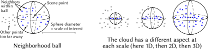
Figure 2: Neighborhood ball at different scales. In this representation, outside points (gray stars) can be on the side but also behind the neighborhood ball.

Let $\lambda_{i},i=1\ldots 3$ be the eigenvalues resulting from the PCA, ordered by decreasing magnitude: $\lambda_{1}\geq\lambda_{2}\geq\lambda_{3}$. The proportion of variance explained by each eigenvalue is $p_{i}=\frac{\lambda_{i}}{\lambda_{1}+\lambda_{2}+\lambda_{3}}$. Fig. 3 shows the domain of all possible proportions.

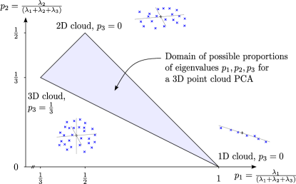
Figure 3: Representing the eigenvalues repartitions for the local neighborhood PCA in a triangle.

When only a single eigenvalue $\lambda_{1}$ accounts for the total variance in the neighborhood ball the points are distributed only in one dimension around the reference scene point. When two eigenvalues are necessary to account for the variance but the third one does not contribute the cloud is locally mostly two-dimensional. Similarly a fully 3D cloud is one where all three eigenvalues have the same magnitude. The proportions of eigenvalues thus define a measure of how much 1D, 2D or 3D the cloud appears locally at a given scale (see Figs. 2 and 3). Specifying these proportions is equivalent to placing a point $X$ within the triangle domain in Fig. 3, which can be done using barycentric coordinate independently of the triangle shape. Given the constraint $p_{1}+p_{2}+p_{3}=1$, a two-parameter feature for quantifying how 1D/2D/3D the cloud appears can be defined at any given point and scale.

A related measure has been previously introduced for natural terrain analysis in the context of ground robot navigation [45, 23] and urban lidar classification [9]. In these applications, the eigenvalues of the PCA are used only as ratios that are compared to three thresholds in order to define the feature space. In the present study we not only consider the full triangle of all possible eigenvalue proportions, as shown in 3, but also span the feature over multiple scales. The “tensor voting” technique from computer vision research predates our work in its use of eigenvalues to quantify the dimensionality of the lidar data cloud [38, 20], although with a different algorithmic approach. Our work is to our best knowledge the first to combine the local dimensionality characterization over multiple scales. We chose PCA as it is a simple and standard tool for finding relevant directions in the neighborhood ball [40]. Other projections techniques (e.g. non-linear) could certainly be used for defining different descriptors of the neighborhood ball geometry, but our results below show that PCA is good enough already.

3.2 Multiple scales feature

The treatment described in the previous section is repeated at each scale of interest (see Fig. 2). Given $N_{s}$ scales, we thus get for each point in the scene a feature vector with $2.N_{s}$ values. This vector describes the local dimensionality characteristics of the cloud around that point at multiple scales. In the context of ground based lidar data there may be missing scales, especially the smallest ones, because of reduced point density, nearby shadows or scene boundaries. In that case the geometric properties of the closest available larger scale is propagated to the missing one in order to complete the $2.N_{s}$ values. Fig. 4 shows an example of how a scene appears using this representation for 4 scales.

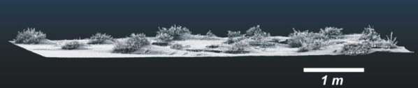
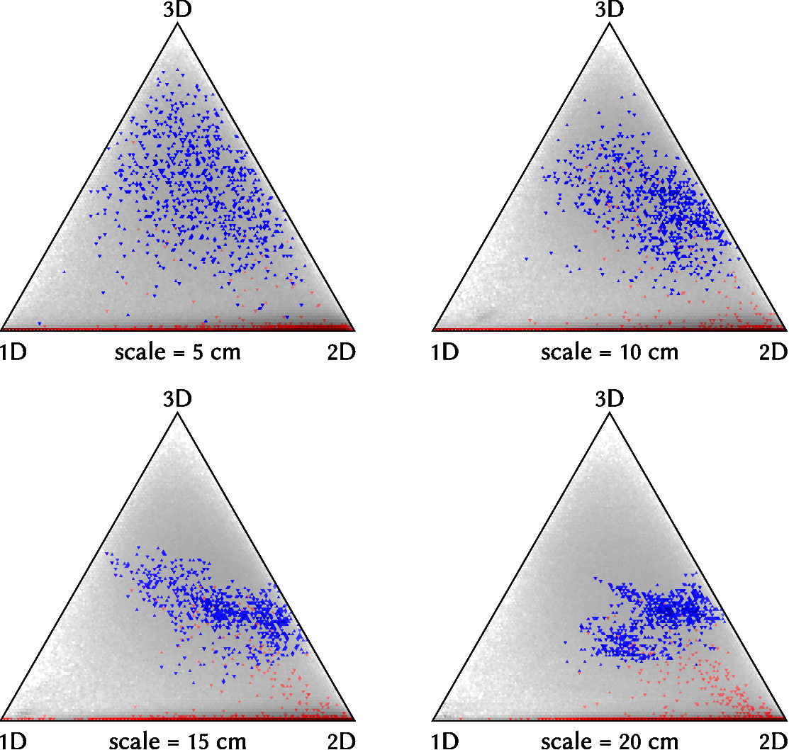
Top : excerpt from a point cloud acquired in the Mont Saint-Michel bay salt marshes (Fr), in a zone of pioneer riparian vegetation and sand (point spacing from 2.3 to 14 mm). Bottom (with color available online): Dimensionality density diagrams for one vegetation patch (blue, appearing as dark gray when printed as gray), a patch of ground (red, appearing as dark gray on the triangles bottom right 2D region), and all other points of the scene (light gray). Each triangle is a linearly transformed version of the space in Fig. 3 at the indicated scale. Each corner thus represents the tendency of the cloud to be respectively 1D, 2D, or 3D.

Figure 4: Density plots of a scene represented in the proposed feature space at different scales.

Note how a single patch of vegetation (in blue in Fig. 4) defines a changing pattern at different scales, but remains separated from the ground (in red), hinting at a classification possibility. However the rest of the scene (unlabeled, gray points) is spread through the whole triangle at each scale: there is no clear cut between vegetation and ground at any given scale. The solution is brought by considering the multiscale vector in its entirety, as a high-dimensional description, and not as a succession of 2D spaces. This is described in the next section.

4 Classification

The general idea behind the classification procedure is to define the best combination of scales at which the dimensionality is measured, that allows the maximum separability of two or more categories. Practically, the user could have an intuitive sense of the range of scales at which the categories will be the most geometrically different, but in many cases, because of natural variability in shape and size of objects, this is not a trivial exercise. We thus rely on an automated construction of a classifier that finds the best combination of scales (i.e. all scales contribute to the final classification but with different weights) that maximizes the separability of two categories that the user has previously manually defined (i.e. samples of vegetation and samples of ground segmented from the point cloud). In the following we describe the construction of the classifier and then present in section 5 typical classification results and step-by-step application to natural data sets.

4.1 Probabilistic classifier in the plane of maximal separability

The full feature space of dimension $2.N_{s}$ is now considered in order to define a classifier that takes advantage of working simultaneously on the data representation at multiple scales. This classifier is defined in two steps: 1. by projecting the data in a plane of maximal separability; and 2. by separating the classes in that plane. The main advantage of processing this way is to get an easy supervision of the classification process. Visual inspection of the classifier in the plane of maximal separability is very intuitive, which in turn allows for an easy improvement of the classifier if needed (e.g. changing the separation line in Fig. 5 to make a non-linear classifier).

The plane of maximal class separability is intuitively like a PCA where only the 2 main components are kept, except that it optimizes a class separability criterion instead of maximizing the projected variance as the PCA would do. In principle any classifier allowing a projection on a subspace can be used in an iterative procedure (including non-linear classifiers with the kernel trick, see [27]). In the present work two linear classifiers are considered: Discriminant Analysis [44] and Support Vector Machines [7]. The rational is to assert the usefulness of our new feature for discriminating classes of natural objects. Comparing the results obtained with these two widely used linear classifiers validates that the newly introduced feature does not depend on a complex statistical machinery to be useful. We stress that last point: using one or the other of these classifiers has little impact in practice (see the results in section 5.1), but we had to demonstrate this is actually the case and that using a simple linear classifier is good enough for our use.

Let $F=\left\{X=(x_{0},y_{0},x_{1},y_{1},\ldots,x_{Ns},y_{Ns})\right\}$ be the multiscale feature space of dimension $2.N_{s}$, with $(x_{i},y_{i})$ the coordinates within each triangle in Fig. 4. Consider the set of points $F^{+}$ and $F^{-}$ labeled respectively by $+1$ or $-1$ for the two classes to discriminate (ex: vegetation against ground). A linear classifier proposes one solution in the form of an hyperplane of $F$ that best separates $F^{+}$ from $F^{-}$. That hyperplane is defined by $w^{T}X-b=0$ with $w$ a weight vector and $b$ a bias:

• Linear Discriminant Analysis proposes to set $w=\left(\Sigma_{1}+\Sigma_{2}\right)^{-1}\left(\mu_{2}-\mu_{1}\right)$ where $\Sigma_{c}$ and $\mu_{c}$ are the covariance matrix and the mean vector of the samples in class $c$.

• Support Vector Machines set $w$ so as to maximize the distance to the separating hyperplane for the nearest samples in each class. The Pegasos approach described in [39, 21] is used here to compute $w$ since it is adapted to cases with large number of samples while retaining a good accuracy.

In each case the bias $b$ is defined using the approach described in [33], which gives a probabilistic interpretation of the classification: the distance $d$ of a sample to the hyperplane corresponds to a classification confidence, internally estimated by fitting the logistic function $p(d)=\frac{1}{1+exp(-\alpha d)}$.

The feature space $F$ is then projected on the hyperplane using $w$ and $b$, and the distance to the hyperplane $d_{1}=w_{1}^{T}X-b_{1}$ is calculated for each point. The process is repeated in order to get the second-best direction orthogonal to the first, together with the second distance $d_{2}$. The couple $(d_{1},d_{2})$ is then used as coordinates defining the 2D plane of maximal separability. Since there is a degree of freedom in choosing $w,b$ such that $w^{T}X-b=0$, both axis can be rescaled such that $\alpha=1$. Thus the coordinates $(d_{1},d_{2})$ in the separability plane are now consistent in classification accuracy. This consistency allows some post-processing in the plane. With the current definition most classifiers would squash the data toward the $X=Y$ diagonal. The post-processing consists in rotating the plane so that the class centers are aligned on X, and then scaling the Y axis so the classes have the same variance on average in both direction. This last step is completely neutral with respect to the automated classifier that draws a line in the plane (the optimal line could be defined whatever the last rotation and scaling). However it is now much easier to visually discern patterns within each class in the new rotated and rescaled space, as can be seen is Fig. 5.

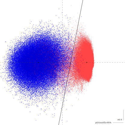
Color is available online. Blue (dark gray): vegetation samples. Red (light gray): soil. The classifier was obtained automatically with a linear SVM using the process described in Section 4.1 in order to classify the benchmark described in Section 5.1. The confidence level is given for the horizontal axis. The scaling for the Y axis has no impact on the automated classification performance but offers a better visualization, which is especially useful when the user wishes to modify this file graphically.

Figure 5: Classifier definition in the plane of maximal separability.

That figure shows an example of classifier automatically obtained using the data presented in Section 5.1. The given scale of 95% classification confidence is valid along the X axis and the corresponding factor for the Y axis is indicated.

4.2 Semi-supervised learning

One goal in developing this classification method was to minimize user input (i.e. manually extracting and labeling data in the scene is cumbersome) while maximizing the generalization ability of the classifier . This is achieved by semi-supervised learning: using the information which is present in the unlabeled points. The plane of maximal separability is necessarily computed only with the labeled examples. We search for a direction in this plane which minimizes the density of all points along that direction (labeled and unlabeled), while still separating the labeled examples. The assumption is that the classes form clusters in the projected space, so minimizing the density of unlabeled points should find these clusters boundaries. When no additional unlabeled data are present the classes are separated simply with a line splitting both with equal probability.

For a multi-class scenario (see Section 5.2) the final classifier is a combination of elementary binary classifiers. In that case it may be that some cluster in the unlabeled data corresponds to another class than the two being classified, which would fool the aforementioned density minimization. A workaround is to use only the labeled examples, or to rely on human visual recognition to separate the clusters manually.

More generally the ability to visualize and keep control of the process (this is not a “black box” tool) allows to tap on human perception to better separate classes. But the ability to fully automate the operations is retained, which is especially useful for large batch processing. The user can always review the classifier if needed.

We developed a tool usable by non-specialists: the classifier is provided in the form of a simple graphics file that the user can edit with any generic, commonly available SVG editor. The decision boundary can be graphically modified, thus quickly defining a very powerful classifier with minimal user input. This step is fully optional and the default classifier can of course be taken without modification.

4.3 Optimization

The most time-consuming parts of the algorithm are computing the local neighborhoods in the point cloud at different scales in order to apply the local PCA transform (see Section 4.1), as well as the SVM training process (computing the Linear Discriminant Analysis is fast and not an issue, although even when using a SVM, training a classifier is only needed once per type of natural environment). We address these issues by allowing to compute the multiscale feature on a sub-sampling of the scene called core points. The whole scene data is still considered for the neighborhood geometrical characteristics, but that computation is performed only at the given core points.

This is a natural way of proceeding for lidar data: given the inhomogeneous density there is little interest in computing the multiscale feature at each point in the densest zones. A spatially homogeneous density of core points is generally sufficient and allows an easier scene manipulation and visualization. However the extra data available in the densest zones is still used for the PCA operation, which results in increased precision compared to far away zones with less data points. We also preserve the local density information and the classification confidence around each core point as a measure of that precision. When classifying the whole scene, each scene point is then given the class of the nearest core point.

As a result the user is offered a trade-off between computation time and spatial resolution : it is possible to call the algorithm on the whole scene (each point is a core point) or to call the algorithm on a sub-sampling of the user choice (e.g., an homogeneous spatial density of core points).

5 Results

5.1 Quantitative benchmark on ground and riparian vegetation classification

In order to quantitatively assess the performance of the classifier, examples were selected from the pioneer salt marsh scene (see Fig. 4 for an excerpt of this scene) in which two classes can be defined : riparian vegetation and ground. These examples represent various vegetation patch sizes and shapes, shadow zones, flat ground, small ripples, data density changes and multiple scanner positioning. The data set comprises approximately 640000 points, manually classified into 200000 belonging to vegetation and 440000 for ground. This data set is provided online together with the software (link given at the end of this paper) so it can be reused for comparative benchmarks.

The classifier is trained to recognize vegetation from ground in the first set of examples, using about half of the aforementioned data. Its performance is then assessed on a the remaining half of the data that was not used for training. This is not only the standard procedure in the machine learning field (to detect when the algorithm learns details of a particular data set that are not transposable to other data sets, i.e. the over-fitting issue), but also what is expected from our new technique. We aim at an excellent generalization ability: the algorithm must be able to recognize the vegetation in unknown scenes, not only just on the samples it was presented.

We use the balanced accuracy measure to quantify the performance of the classifier in order to account for the different number of points in each class. With $tv,\,tg,\,fv,\,fg$ the number of points truly($t)$/falsely($f$) classified into the vegetation($v$)/ground($g$) classes, the balanced accuracy is classically defined as $ba=\frac{1}{2}\left(a_{v}+a_{g}\right)$ with each class accuracy defined as $a_{v}=\frac{tv}{tv+fg}$ and $a_{g}=\frac{tg}{tg+fv}$. We use the Fisher Discriminant Ratio $fdr$ [44] in order to assess the class separability. The classifier assigns for each sample a signed distance $d$ to the separation line, using negative values for one side and positive values for the other. The measure of separability is defined as $fdr=\left(\mu_{2}-\mu_{1}\right)^{2}/\left(v_{1}+v_{2}\right)$ with $\mu_{c}$ and $v_{c}$ the mean and variance of the signed distance $d$ for each class $c$. Note that the class separability could still be high despite a mediocre accuracy (e.g., separation line positioned on a single side from both classes). This would merely indicate a bad training with potential for a better separation. Hence both $ba$ and $fdr$ are useful measures for asserting separately the role of the classifier and the role of the newly introduced feature in the final classification result. A large $ba$ value indicates a good recognition rate ($ba=50\%$ indicates random class assignment) on the given data set, and a large $fdr$ value indicates that classes are well separated (an indication that the $ba$ score is robust).

LDA classifier		Accuracy	$ba$	$fdr$
Training set	Vegetation	98.3%	97.9%	12.3
	Ground	97.6%
Testing set	Vegetation	99.3%	97.6%	11.0
	Ground	95.9%

SVM classifier		Accuracy	$ba$	$fdr$
Training set	Vegetation	98.7%	98.0%	11.1
	Ground	97.3%
Testing set	Vegetation	99.6%	97.5%	11.0
	Ground	95.4%

The performances of each classifier is measure using the Balanced Accuracy (ba) and the Fisher Discriminant Ratio (fdr). Both are described in the main text.

Table 1: Quantitative benchmark for separating vegetation from ground.

Table 1 shows the results of the benchmark. The classifier that was used is fully automated, without human intervention on the decision boundary, and taking 19 scales between 2cm and 20cm every cm (larger scales do not improve the classification, see Fig. 5 for the typical vegetation size $\approx 40$cm). We used our software default quality / computation time trade-off for the support vector machine classifier training in order to adequately assess the results of our algorithm in usual conditions. The algorithm was forced to classify each point, while in practice the user may decide to ignore points without enough confidence in the classification (see Section 5.2). Nevertheless the balanced accuracy that was obtained both on the training set and the testing set is very good. This not only shows that the algorithm is able to recover the manually selected vegetation/soil (train set accuracy) but that it is able to generalize to terrain data it had not seen before. This is of great importance for large campaigns: we can train the algorithm once on a given type of data and then apply the classifiers to a large quantity of further measurements without having to re-train the algorithm.

LDA and SVM	5cm		10cm		15cm		20cm
	$ba$	$fdr$	$ba$	$fdr$	$ba$	$fdr$	$ba$	$fdr$
Training	97.0%	5.2	97.1%	6.5	96.6%	5.6	95.7%	4.6
Testing	97.3%	6.4	96.9%	6.5	95.7%	4.8	94.1%	3.7

The results for both classifiers differ only at the fourth digit for the Balanced Accuracy ($ba$) and at the third for the Fisher Discriminant Ratio ($fdr$), so the tables were merged.

Table 2: Single scale benchmark results at selected scales

Table 2 shows the result of the classification using single scales only. The advantage of using a multi-scale classifier is apparent: it offers a better accuracy than any single scales alone. The difference is more pronounced for the discriminative power, with the multi-scale classifier offering almost twice as much class separability. Although this is the expected behavior, some classifiers are sensitive to noise and adding scales with no information would potentially decrease the multi-scale performance. The scales from 2cm to 20cm not shown in Table 2 have similar properties and performance levels, with slightly better results for single scales between 5 and 10 cm. Even with this observed performance peak there is no characteristic scale in this system as discriminative information is present at all scales: the point of the multi-scale classifier is precisely to exploit that information.

In this example, both classifiers (LDA and SVM) give the same results at each scale, and are equally suitable for the multiscale feature (Table 1). In other scenarios the situation might be different, but overall this confirm our method does not need a complicated statistical machinery (like the SVM) for being effective, and using a simple linear classifier (like the LDA) is good enough. In any case we achieve at least 97.5% classification accuracy.

Figure 6 visually shows the result of the classification on a subset of the test data using the multi-scale SVM classifier obtained with the fully automated procedure. Points with a low classification confidence are highlighted in blue. They correspond mostly to the boundary between ground and vegetation. Figure 6 shows that the algorithm copes very well with the irregular density of points, the shadow zones and the ripples. The actual classifier definition is shown in Fig. 5.

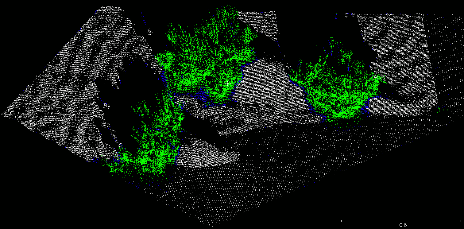
Color is available online. White: Points recognized as ground. Green (light gray): Points recognized as vegetation. Blue(dark gray): Points for which the confidence in the classification is less than 80%. Scale is in meters.

Figure 6: Excerpt of the quantitative benchmark test set classification

5.2 3D multiscale classifiers with multiple classes

5.2.1 Dealing with multiple class

Combining multiple binary classifiers into a single one for handling multiple classes is a longstanding problem in machine learning [41]. Typically the problem is handled by training “one against one” (or “one against others”) elementary binary classifiers, which are then combined by a majority rule. This is what the automated tool suite CANUPO proposes in the present context, following the common practice in the domain.

Additional extensions are of course possible in future works. Recent developments on advanced statistical techniques [41] deal with the issue of training and then combining the elementary classifiers. However in the present context we wish to retain a possible intervention on the classifiers using a graphical editor. Moreover context-dependent choices like favoring one class over the other need to be allowed. It may thus be more efficient to separate classes one by one and combine the results, as is explained in the next section.

5.2.2 Application to a complex natural environment

In the following we illustrate the capabilities of the method in classifying complex 3D natural scenes. A subset of the Otira River scene (fig. 1) was chosen, and four main classes defined: vegetation, bedrock surface (on the channel bank and large blocs), gravel surfaces and water. Figure 7 presents the dimensionality density diagrams of one training patch for each class and scales ranging from 5 to 50 cm. As intuitively expected, vegetation is mostly 1D and 2D at small scale (leaves, stem) and becomes dominantly 3D at scales larger than 15 cm. However, the clustering of points is only significant at scales larger than 20 cm. Bedrock surfaces are mostly 2D at all scales, with some 1D-2D features occurring at fine scales corresponding to fractures. Gravel surfaces exhibit a larger scatter at all scales owing to the large heterogeneity in grain sizes. The 3D component is more important at intermediate scales (10 to 20 cm) than at small or very large scales. This illustrates the transition from a scale of analysis smaller than the dominant gravel size (i.e., gravels appears as dominantly 2D curved surfaces), and then larger than an assemblage of gravels (i.e., gravel roughness disappears). As explained in section 2, whitewater surface can be picked by the laser, whereas in general it does not reflect on clear water [28]. Yet, even at small scale the water does not appear purely 2D as the water surface is uneven and the laser penetrates at different depth in the bubbly water surface. Indeed, the signature is quite multidimensional for scales up to 20 cm, and only around 20 cm does the water surface appear to significantly cluster along a 2D-3D dimensionality. At larger scale, the water becomes significantly 2D.

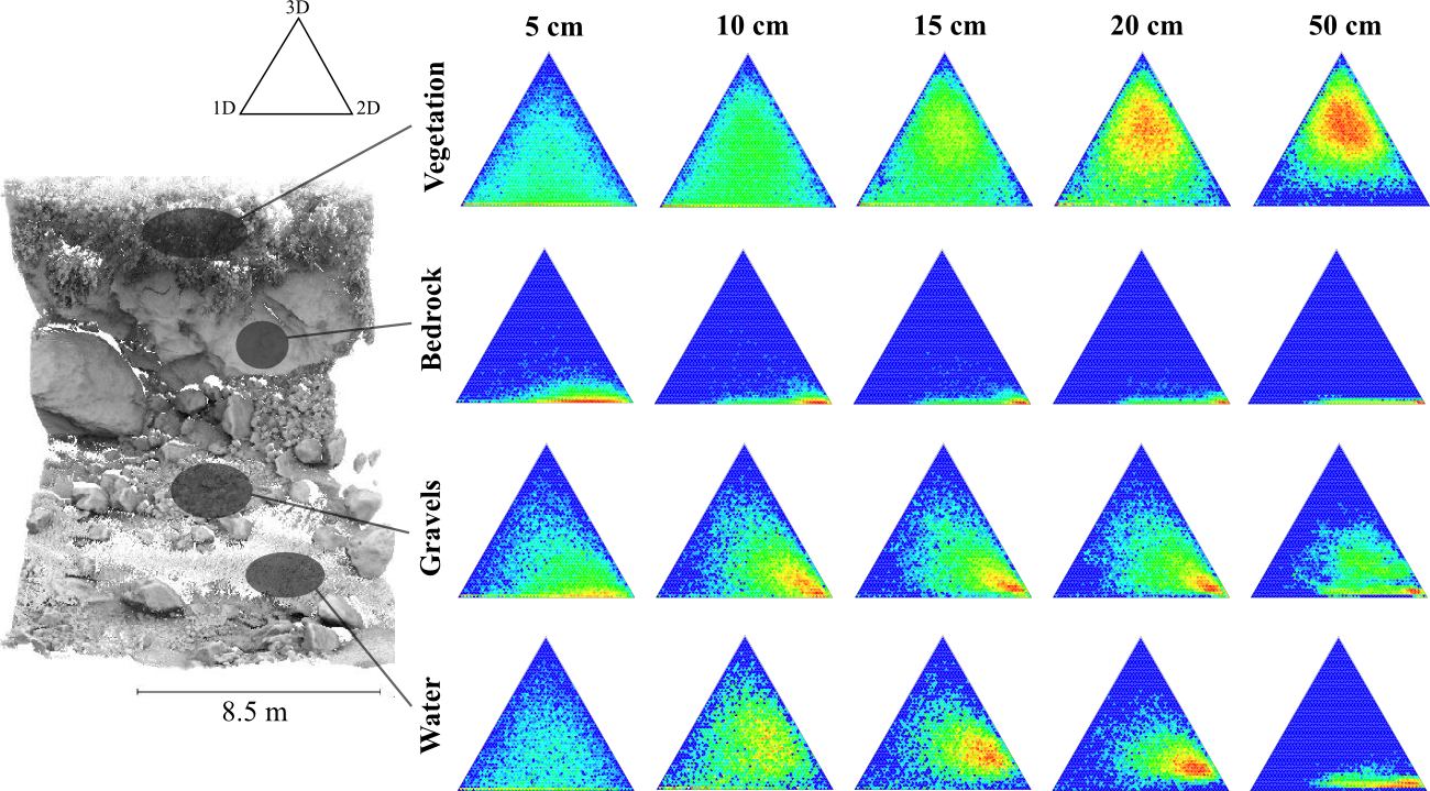
Figure 7: Multiscale, multi-class scenario

Left : excerpt from the point cloud of fig. 1. Right: dimensionality diagrams for the four main classes of a mountain river environment at scales ranging from 5 to 50 cm. Colors from blue to red correspond to the density of points from the training dataset and characterize the degree of clustering around a given dimensionality.

The multi-scale properties of the various classes show that there is not a single scale at which the classes could be distinguished by their dimensionality. Vegetation and bedrock are quite distinct at large scale, but bedrock, gravel and water are too similar at this scale to be labeled with a high level of confidence. Only at smaller scales (10-20 cm) can bedrock be distinguished from gravel and water. This visualization also shows that gravel and water will be difficult to distinguish owing to their very similar dimensionality across all the scales.

In the following, approximatively 5000 core points for each class were selected for the training process. Their multiscale characteristics were estimated using the complete scene rather than excerpts of the class only. Points in the original scene have a minimal spacing of 1 cm corresponding to ~ 1.17 million points. The actual classification operates on subset of 330000 core points with a minimum spacing of 2 cm. The multi-classes labeling was achieved using a series of 3 binary classifiers (fig. 8) all using the same set of 22 scales (from 2 cm to 1 m). An automated classification (i.e., the only user interaction was in defining the classes and the initial training sets) is presented, as well as examples of possible user alterations.These alterations are of three types : changing the initial training sets, modifying the classifier, and defining a classification confidence interval. Given that users improvements depend on specific scientific objectives (e.g., documenting vegetation, characterizing grain sizes or measuring surface change), they cannot all be discussed completely here. We present a case in which the classification of bedrock surfaces was slightly optimized. The LDA approach was used for all classifier definitions as the results were on par or slightly better than a SVM approach. Figure 9 presents the results for the original data, the automated and the user-improved classification results.

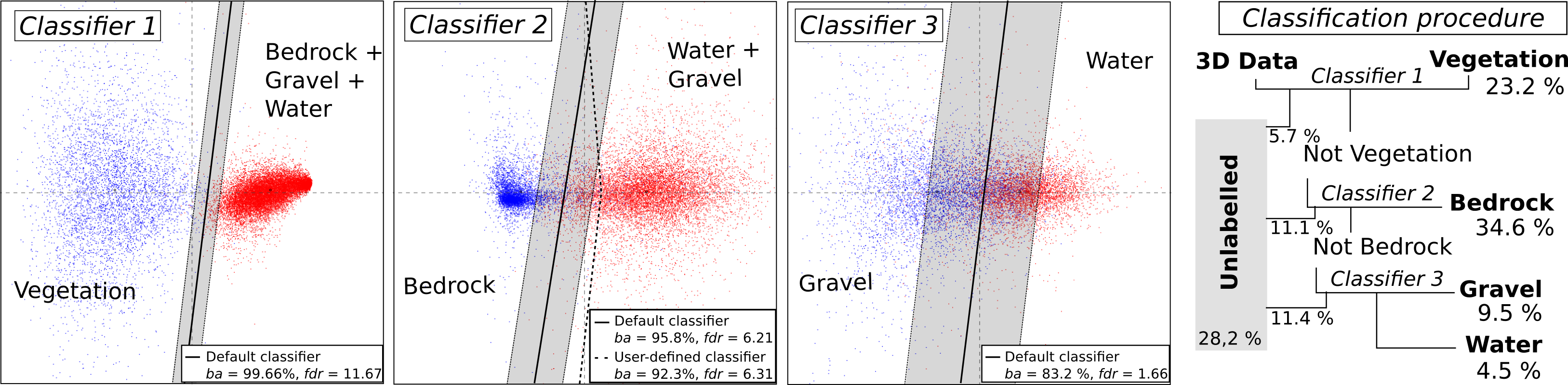
Figure 8: Classification process and classifiers for the multiscale case

Semi-supervised classifiers for the Otira river dataset and classification procedure diagram. For each classifier, the gray area indicates the portion of space in which the classification confidence is lower than 0.95. For Classifier 2, the manually modified supervised classifier is targeted to preserve more systematically bedrock surfaces at the expense of non-bedrock surfaces. In the classification procedure diagram, percents indicate the proportion of each class in the supervised classification which uses confidence intervals of 0.9 for Classifier 1, 0.8 for Classifier 2 and Classifier 3.

The first classifier separates vegetation from the three other classes. The automated training procedure results in a $ba$ of 99.66 % approaching perfect identification of vegetation on the training sets. The very high level of separability is reflected by a large $fdr$ value (11.67) and a very small classification uncertainty in the projected space (fig. 8). As shown in figure 9, the automated classification of vegetation is excellent with very limited false positives appearing in overhanging parts of large blocs where the local geometry exhibits a dimensionality across various scales too similar to vegetation. The precision of the labeling is also excellent as small parts of bedrock between or behind vegetation are correctly identified, and small shrubs are correctly isolated amongst bedrock surfaces. Nevertheless it is still possible to improve this classifier by using the incorrectly classified overhanging blocs in the training process (5000 core points were added). This 5 minutes operation results in a better handling of false vegetation positive, and retains excellent characteristics on the original training sets ($ba$ = 98.2 %, $fdr$ = 9.89). A classification confidence interval of 90 % was also set visually in the CloudCompare software [12] by displaying the uncertainty level of each core point and defining the optimum between quality and coverage of the classification. This left aside 5.7 % of the original scene points unlabeled.

Classifier 2 separates bedrock surfaces from water and gravel surfaces (fig. 8). The automated training procedure lead to a $ba$ of 95.7 % and $fdr$ of 6.21 on the original training sets. Because gravels exhibits a wide range of scales from pebbles to boulders, it is not possible to fully separate the bedrock and gravel classes as the largest gravels tend be defined as rock surfaces. Fracture and sharp edges of blocs tend to be classified as non-bedrock as they are 3D feature at small scale and 2D as large scale (as is gravel). Yet, as in the previous case, the confidence level defined at 0.95 remains small compared to the size of the two clusters in the projected space. While the original classifier was already quite satisfactory, it was tuned to primarily isolate rock surfaces by changing manually the classifier position in the hyperplane projection ($ba$ = 92.3 %, $fdr$ = 6.31 ,fig. 8). A classification confidence interval of 80 % was also used which left 17 % of the remaining points unlabeled (fig. 9).

Classifier 3 separates water from gravel surfaces (classifier 3, fig. 8).The automated training procedure lead to a ba of 83,2 %. As expected from the similarity of the dimensionality density diagrams (fig. 7), the two classes are more difficult to separate than in the previous two classifications and the confidence level defined at 0.95 overlaps significantly the two classes. Yet, figure 9 shows that the classifier manages to correctly label the whitewater and gravel surfaces corresponding to non-trained datasets. Being quite effective, the default classifier was not altered. A confidence interval of 80 % was used resulting in 78 % of the remaining points being labeled.

The end result of this process is a 3D scene (fig. 9). As shown in fig. 9 the default parameters already give an excellent first order classification. The fine-tuning previously described do not represent the best classification possible, but rather an example of how the automated approach can be rapidly tweaked to give some improvement. On a practical note, the simplest way to improve the default classifier in this example is to add in the training process some of the false positive and false negative results of a first training, rather than manually altering the classifier. Defining a confidence level during the classification process is very useful as the amount of data is so large that labeling only 70 % of the points is not detrimental to the interpretation of the results. The classes can be further cleaned by removing isolated points using the volumetric density of data calculated during the multi-scale analysis.

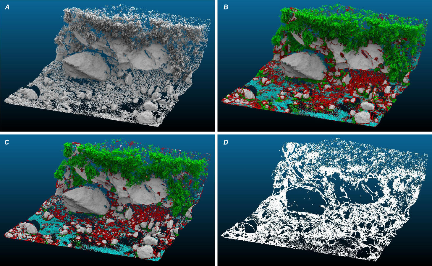
Figure 9: Result of the classification process for the mountain river dataset

A: Original Otira River scene (minimum point spacing = 1 cm). B: Default classification (green: vegetation, gray: bedrock, red: gravel, blue: water) according to the process described in fig. 8. C : User-improved classification. D : unlabeled points (28,2 % of the total points).

5.3 Single scale vs Multiple scale classification

Table 3 presents the balanced accuracy of the three classifiers used in the Otira river scene (fig. 8) trained with the same subsets but using a single spatial scale (5, 10, 20, 50, 75 or 100 cm). For each classifier, the balanced accuracy of the multiple scale classification is systematically better than the single scale ones. The improvement is very significant for Classifier 3 (83.2 % vs 70.9 % for single class). Most importantly, the separability of classes (as measured by the $fdr$) is always increased at least two to three times for Classifiers 2 and 3 (and by 40 % for Classifier 1). The increased separability is the key advantage of the multi-scale approach. It allows a larger geometrical inhomogeneity within a given class, and a better generalization of the results than a single scale approach.

Compared to a single scale classification at 1 m, the improvement of the multi-scale Classifier 1 (vegetation vs not vegetation) seems more marginal. However, by comparing the classification results on the Otira river data, the multi-scale classifier is more precise than the single-scale case: small shrubs within bedrock, that are not correctly classified by the single large scale classifier, are correctly retrieved with the multi-scale approach. Similarly, incorrectly classified zones below blocs for both classifiers are more extended with the single-scale classifier. Therefore the multi-scale classification is qualitatively improved, which is not reflected by the quantitative $ba$ measure alone.

We conclude that the multi-scale analysis always improve significantly the classification compared to a single scale analysis on one or all of the following aspects : discrimination capacity, separability of the classes and spatial resolution.

Scale	Classifier 1		Classifier 2		Classifier 3
(cm)	vegetation		bedrock		water,gravel
	$ba$ %	$fdr$	$ba$ %	$fdr$	$ba$ %	$fdr$
2-100	99.66	11.67	95.7	6.21	83.2	1.66
5	67.51	0.18	78.75	1.04	70.28	0.32
10	58.6	0.03	88.47	1.89	69.36	0.46
20	82.23	1.76	92.15	2.84	62.03	0.14
50	95.59	5.73	85.24	1.56	68.28	0.41
75	98.24	7.55	79.85	1.03	69.85	0.43
100	98.98	8.2	78.74	0.77	70.9	0.50

Table 3: Comparison of Balanced Accuracy on Single scale and Multi-scale classifier

Results of semi-supervised LDA classification for single and multiple scales using the original training sets of the Otira river classifiers (fig. 8). Results are similar using an SVM approach.

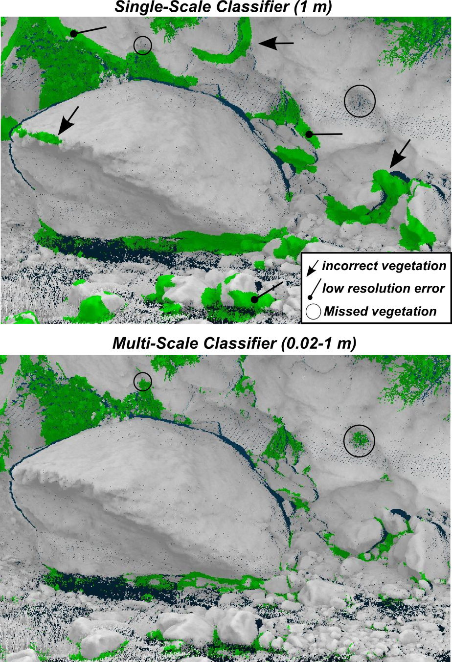
Figure 10: Comparison of best single scale vegetation classifier with multi-scale classifier

Classification results for vegetation detection using a multi or single scale (1 m) classifier. Even though the balanced accuracy is similar on the training set the multi-scale classification is much more precise and less prone to errors when generalized to the whole scene. The single scale classifier misses small shrubs on the bedrock and incorrectly classify large bloc borders as vegetation.

6 Discussion / openings

While many studies have focused on the classification of ground vs vegetation, or buildings in 2.5D airborne lidar data using purely geometrical approaches (e.g., [42, 3, 9]), none can really apply to dense 3D point clouds obtained from ground based (fixed or mobile) lidar data in which a fully 3D approach is needed. Such 3D approach have been pursued using a dimensionality measurement at a given scale [45, 23] to detect 1D (e.g. tree trunk or cables), 2D (ground) and 3D (vegetation) objects. However, because natural surfaces exhibit a large range of characteristic scales and natural objects within a given class can have a large degree of geometric heterogeneity (i.e. vegetation or sediment), a single scale can rarely classify an entire scene robustly. We have thus introduced a multi-scale analysis of the local geometry of point clouds to cope with the aforementioned issues, which exhibits good performance even with simple linear classifiers. By doing so the selection of a specific or characteristic scale is not needed. We have shown that the combination of scales systematically improves the separability of classes compared to a single scale analysis (Table 3, Table 1 vs Table 2), sometimes dramatically. The multi-scale analysis also allows retention of a detailed spatial resolution compared to a single large scale analysis. To further account for the geometrical complexity of natural environments, the user is free to set a level of confidence in the classification process that will control the balance between confidence and coverage of the classification. Given the large amount of data available in TLS, it is often more interesting to not classify 30 % of the data, in order to keep 70 % for which classes are correctly attributed.

Because all scales contribute to a varying degree to the classification process, the method is relatively robust to shadow effects, missing data and irregular point density (e.g. fig. 9b and 6): even if the dimensionality cannot be characterized over a certain range of scales (e.g. small ones because of low point density, large ones because of shadow effects), other scales are used to classify a point, albeit with a smaller degree of confidence. Interestingly, qualitative inspection of the classification results shows that obvious spurious mixed points created at the edge of objects tend to be classified with a low level of confidence (provided that the scene has a relatively high point density and that the small scale dimensionality significantly contribute to the classification). This is explained by the low point density around mixed points (because no real object exists at their location) and the resulting lack of a good dimensionality characterization at small scale. Although systematically quantifying this effect if out of the scope of this work, this observation suggests that using a relatively high level of confidence during the classification process helps in cleaning the resulting classes from spurious mixed-points.

We chose the dimensionality of the point cloud at a given scale as a continuous measure of the local scene geometry. This is an intuitive perception of the surface that can capture many aspects of natural geometries ([45, 23]), in particular the dichotomy between 3D vegetation and 2D surfaces. However, the multi-scale classification could also use other geometrical measures depending on the final objectives of the classification. Surface orientation, curvature, mathematical derivatives of a local surface [6] or the degree of conformity to a given geometry (sphere, cylinder ….e.g., [46]) could also have been used in the construction of the classifier. The surface angle with the vertical is already implemented in the classifier but was not used here. It could be used to separate channel banks from river bed for instance, or as an additional constraint to discriminate the water surface from the gravels (which are rarely completely horizontal compared to water). We note that for vegetation classification, the dimensionality measurement is particularly effective and simple to define for 3D point clouds. Indeed, even at a single well chosen scale, the dimensionality criteria performs already well to detect vegetation (i.e., fig. 10)([45, 23]).

Each point captured by lidar (airborne or terrestrial) also comes with a measure of the reflected laser intensity and in some cases with optical imagery information (RGB) that could be used in the classification process. Using the reflected laser intensity for classification purposes has been attempted for airborne (e.g. [14, 18]) and ground-based lidar [11, 32, 24, 13, 19]. In this latter case, the difficulties are numerous as the reflected intensity is a complex function of distance from the scanner, incidence angle, and surface reflectance [19, 24] (which on top of the physico-chemical characteristics of the material itself, also depends on surface humidity and micro-roughness [11, 31, 32]). In simple cases for which the distance and the incidence angle are not greatly changing (cliff survey for instance), the laser intensity can be used to distinguish between materials relatively efficiently [11]. It can also improve the robustness of a classifier based on simple geometrical parameters ([13]) in the case of simple natural environments such as riparian vegetation over sand. However, for complex scenes such as the Otira river, lidar intensity is more difficult to use given the large changes in distances, incidence angles and state of the surface (wet vs dry surfaces). Moreover, no standard exists between scanner manufacturers such that even if surface reflectance could be isolated from other effects, it would not necessarily be comparable between various scanner measurements as opposed to purely geometrical descriptors that can be used for any source of data (i.e. classifiers can be exchanged between users independently of the scanner used to acquire the data). Because laser reflected intensity is not globally nor temporally consistent on a complex 3D scene, we conclude that it cannot yet be used as a primary classifier of complex 3D natural scenes. Development of precise geometrical corrections factors for reflected intensity (e.g., [19]) may allow its future inclusion in the process of classifier training and subsequent classification to improve the resolution and accuracy of the geometrical classification. Provision for this is already included in the software.

In the case of airborne lidar, the combination of geometrical information and imagery can significantly increase classification quality (e.g. [10]). However, RGB imagery have rarely been used in the context of 3D terrestrial lidar classification [24]. The main reason is that it is much more difficult to have a spatially consistent RGB imagery of a 3D complex scene from the ground than from air. Indeed, the more 3D and complex is an outdoor scene, the more difficult it is to get a consistent exposure from the ground and from different points of view. For instance, in the case of the Otira River, the extent of shadows is pronounced owing to the narrow gorge configuration and to the presence of vegetation, and variable during one day. Wetted surfaces which are common in fluvial environments also have a different spectral signature than dry surfaces. Also, RGB imagery cannot distinguish first or last laser reflexions in the case of the new generation of full-waveform multi-echo scanners. However, in the context of the riparian vegetation case example (fig. 6), and owing to the strong difference in spectral characteristics of the vegetation and the sandy bed, good success could be expected using RGB classification [24]. But this requires the imagery to be taken without strong shadows, and in the case of the Leica Scanstation 2 would be limited by the low resolution of the on-board camera and the lack of precise registration with the point cloud (typically a few cm difference at 50 m). Classifying flat versus ripples zones would still require a geometrical analysis.

Because it works in 3D, our method can be used on 2.5D airborne lidar or mostly 2D point clouds ([13, 17, 28, 42]). As shown with the riparian vegetation example, it allows a direct extraction of vegetation on the raw data without the need to construct a raster DEM. Because of the smaller density of points and the smaller range of scales available to characterize trees in full waveform aerial lidar than in ground based lidar, it is not certain that the method will perform significantly better in defining the ground than existing ones for aerial data. However, it should perform well as a generic geometric classifier of surfaces. Although not used in this study, the multiscale calculation also records the vertical angle of the local surface at the largest scale. This could be used as an additional constraint to detect buildings from road for instance.

7 Conclusion

We introduced a new method for classifying 3D point clouds, called multi-scale dimensionality analysis, to characterize features according to their geometry. We demonstrated the applicability of this method in two contexts: 1. separating riparian vegetation from the ground in the Mt St Michel bay, and 2. recognizing rocks, vegetation, water and gravels in a steep mountain river bed. In each case the classification was performed with very good accuracy. The method is robust to missing data and changes in resolution common in ground-based lidar data. By combining various scales, the method systematically performs better than a single scale analysis and improves the spatial resolution of the classification.

Multi-scale dimensionality analysis proves quite efficient especially in separating vegetation from the rest of the data. Removing (or studying) vegetation is a common issue in natural environment studies and this method will be useful in this context given that it can work directly on the raw data. Typical application include bare ground detection to study sedimentation/erosion patterns in fluvial environments ([48]), rock face analysis on which vegetation can grow and create unwanted noise ([22, 37]) or analysis of vegetation patterns and their relation to hydro-sedimentary processes.

We gave a particular attention to provide tools usable by non-specialists of machine learning, while retaining the ability to process large batches of data automatically. This tool set is available as Free/Libre software on the first author home page. Because it relies only on geometrical properties, classifier parameter files can be exchanged between users and applied on any geometrical data without going over the process of training the classifier.

8 Acknowledgments

Daniel Girardeau-Montaut is greatly acknowledged for his ongoing development of the free point-cloud analysis and visualization software CloudCompare [12] used in this work for visualization and point cloud segmentation according to their class. These activities have been carried out with the support of the European Research Executive Agency in the framework of the Marie Curie International Outgoing Fellowship €ROSNZ for D. Lague, and with the support of the RISC-E (Interdisciplinary Research network on Complex Systems in Environment) project for N. Brodu.

References

- [1] A. Abellán, J. M. Vilaplana, and J. Martínez. Application of a long-range terrestrial laser scanner to a detailed rockfall study at vall de núria (eastern pyrenees, spain). Engineering Geology, 88(3-4):136–148, 2006.
- [2] Antonio Abellán, Jaume Calvet, Joan Manuel Vilaplana, and Julien Blanchard. Detection and spatial prediction of rockfalls by means of terrestrial laser scanner monitoring. Geomorphology, 119(3-4):162–171, 2010.
- [3] A. S. Antonarakis, K. S. Richards, and J. Brasington. Object-based land cover classification using airborne lidar. Remote Sensing of Environment, 112(6):2988–2998, 2008.
- [4] A. S. Antonarakis, K. S. Richards, J. Brasington, and M. Bithell. Leafless roughness of complex tree morphology using terrestrial lidar. Water Resources Research, 45(W10401):W10401, 2009.
- [5] A. S. Antonarakis, K. S. Richards, J. Brasington, and E. Muller. Determining leaf area index and leafy tree roughness using terrestrial laser scanning. Water Resources Research, 46:1–12, 2010.
- [6] S. Barnea, S. Filin, and V. Alchanatis. A supervised approach for object extraction from terrestrial laser point clouds demonstrated on trees. The International Archives of the Photogrammetry, Remote Sensing and Spatial Information Sciences, 36(3):135–140, 2007.
- [7] B. Boser, I. Guyon, and V. Vapnik. A training algorithm for optimal margin classifiers. In Fifth Annual Workshop on Computational Learning Theory, COLT ’92, pages 144–152, New York, NY, USA, 1992. ACM.
- [8] P. A. Burrough. Fractal dimensions of landscapes and other environmental data. Nature, 294:240–242, 1981.
- [9] M. Carlberg, P. Gao, G. Chen, and A. Zakhor. Classifying urban landscape in aerial lidar using 3d shape analysis. In 16th IEEE International Conference on Image Processing, pages 1701–1704, 2009.
- [10] Michele Dalponte, Lorenzo Bruzzone, and Damiano Gianelle. Fusion of hyperspectral and lidar remote sensing data for classification of complex forest areas. IEEE Transactions on Geoscience and Remote Sensing, 46(5):1416–1427, 2008.
- [11] Marco Franceschi, Giordano Teza, Nereo Preto, Arianna Pesci, Antonio Galgaro, and Stefano Girardi. Discrimination between marls and limestones using intensity data from terrestrial laser scanner. ISPRS Journal of Photogrammetry and Remote Sensing, 64(6):522–528, 2009.
- [12] D. Girardeau-Montaut. Cloudcompare, a 3d point cloud and mesh processing free software. Technical report, EDF Research and Development, Telecom ParisTech, 2011.
- [13] A. Guarnieri, A. Vettore, F. Pirotti, M. Menenti, and M. Marani. Retrieval of small-relief marsh morphology from terrestrial laser scanner, optimal spatial filtering, and laser return intensity. Geomorphology, 113(1-2):12–20, 2009.
- [14] Hiroyuki Hasegawa. Evaluations of lidar reflectance amplitude sensitivity towards land cover conditions. Bulletin of the Geographical Survey Institute (Japan), 53(6):43–50, 2006.
- [15] G.L. Heritage and D.J. Milan. Terrestrial laser scanning of grain roughness in a gravel-bed river. Geomorphology, 113(1-2):4–11, 2009.
- [16] Rebecca Hodge, James Brasington, and K. Richards. Analysing laser-scanned digital terrain models of grabel bed surfaces: Linking morphology to sediment transport processes and hydraulics. Sedimentology, 56(7):2024–2043, 2009.
- [17] Rebecca Hodge, James Brasington, and K. Richards. In-situ characterisation of grain-scale fluvial morphology using terrestrial laser scanning. Earth Surface Processes and Landforms, 34(7):954–968, 2009.
- [18] B. Hofle and N. Pfeifer. Correction of laser scanning intensity data: Data and model-driven approaches. ISPRS Journal of Photogrammetry and Remote Sensing, 62(6):415–433, 2007.
- [19] Sanna Kaasalainen, Anttoni Jaakkola, Mikko Kaasalainen, Anssi Krooks, and Antero Kukko. Analysis of incidence angle and distance effects on terrestrial laser scanner intensity: Search for correction methods. Remote Sensing, 3(10):2207–2221, 2011.
- [20] Eunyoung Kim and Gérard Medioni. Urban scene understanding from aerial and ground lidar data. Journal of Machine Vision and Applications (IJMVA), 22(4):691–703, 2011.
- [21] Davis E. King. Dlib-ml: A machine learning toolkit. Journal of Machine Learning Research, 10:1755–1758, 2009.
- [22] Richard Labourdette and R. R. Jones. Characterization of fluvial architectural elements using a three-dimensional outcrop data set: Escanilla braided system, south-central pyrenees, spain. Geosphere, 3(6):422–434, 2007.
- [23] Jean-François Lalonde, Nicolas Vandapel, Daniel F. Huber, and Martial Hebert. Natural terrain classification using three-dimensional ladar data for ground robot mobility. Journal of Field Robotics, 23(10):839–861, 2006.
- [24] Derek D. Lichti. Spectral filtering and classification of terrestrial laser scanner point clouds. The Photogrammetric Record, 20(111):218–240, 2005.
- [25] Derek D. Lichti. Error modelling, calibration and analysis of an am-cw terrestrial laser scanner system. ISPRS Journal of Photogrammetry and Remote Sensing, 61(5):307–324, 2007.
- [26] Ee Hui Lim and David Suter. 3d terrestrial lidar classifications with super-voxels and multi-scale conditional random fields. Computer-Aided Design, 41(10):701–710, 2009.
- [27] Tomasz Maszczyk and Włlodzisłlaw Duch. Support vector machines for visualization and dimensionality reduction. In Proceeding of the International Conference on Artificial Neural Networks, LNCS, volume 1, pages 346–356, 2008.
- [28] D. J. Milan, G. L. Heritage, A.R.G. Large, and N.S. Entwistle. Mapping hydraulic biotopes using terrestrial laser scan data of water surface properties. Earth Surface Processes and Landforms, 35(8):918–931, 2010.
- [29] David J. Milan, George L. Heritage, and David Hetherington. Application of a 3d laser scanner in the assessment of erosion and deposition volumes and channel change in a proglacial river. Earth Surface Processes and Landforms, 32(11):1657–1674, 2007.
- [30] S. Nagihara, K. R. Mulligan, and W. Xiong. Use of a three-dimensional laser scanner to digitally capture the topography of sand dunes in high spatial resolution. Earth Surface Processes and Landforms, 29(3):391–398, 2004.
- [31] Joanna M. Nield, Giles F. S. Wiggs, and Robert S. Squirrell. Aeolian sand strip mobility and protodune development on a drying beach: examining surface moisture and surface roughness patterns measured by terrestrial laser scanning. Earth Surface Processes and Landforms, 36(4):513–522, 2011.
- [32] Arianna Pesci and Giordano Teza. Effects of surface irregularities on intensity data from laser scanning: an experimental approach. Annals of Geophysics, 51(5-6):839–848, 2008.
- [33] John C. Platt. Probabilistic Outputs for Support Vector Machines and Comparisons to Regularized Likelihood Methods, pages 61–74. MIT Press, 1999.
- [34] A. Rabatel, P. Deline, S. Jaillet, and L. Ravanel. Rock falls in high-alpine rock walls quantified by terrestrial lidar measurements: A case study in the mont blanc area. Geophysical Research Letters, 35(L10502), 2008.
- [35] F. Renard, C. Voisin, D. Marsan, and J. Schmittbuhl. High resolution 3d laser scanner measurements of a strike-slip fault quantify its morphological anisotropy at all scales. Geophysical Research Letters, 33(L04305), 2006.
- [36] N. J. Rosser, D. N. Petley, M. Lim, S. A. Dunning, and R. J. Allison. Terrestrial laser scanning for monitoring the process of hard rock coastal cliff erosion. Quarterly Journal of Engineering Geology and Hydrogeology, 38(4):363–375, 2005.
- [37] Nick Rosser, Michael Lim, David Petley, Stuart Dunning, and Robert Allison. Patterns of precursory rockfall prior to slope failure. Journal of Geophysical Research, 112(F04014):F04014, 2007.
- [38] Hanns-F. Schuster. Segmentation of lidar data using the tensor voting framework. In International Archives of Photogrammetry Remote Sensing and Spatial Information Sciences, volume 35, pages 1073–1078, 2004.
- [39] S. Shalev-Shwartz, Y. Singer, and N. Srebro. Pegasos: Primal estimated sub-gradient solver for svm. In Proceedings of the 24th international conference on Machine learning, pages 807–814, 2007.
- [40] Peter J. A. Shaw. Multivariate statistics for the environmental sciences. London : Arnold, 2003.
- [41] Yuichi Shiraishi and Kenji Fukumizu. Statistical approaches to combining binary classifiers for multi-class classification. Neurocomputing, 74(5):680–688, 2011.
- [42] G. Sithole and G. Vosselman. Experimental comparison of filter algorithms for bare-earth extraction from airborne laser scanning point clouds. ISPRS Journal of Photogrammetry and Remote Sensing, 59(1-2):85–101, 2004.
- [43] Giordano Teza, Arianna Pesci, Rinaldo Genevois, and Antonio Galgaro. Characterization of landslide ground surface kinematics from terrestrial laser scanning and strain field computation. Geomorphology, 97(3-4):424–437, 2008.
- [44] Sergios Theodoridis and Konstantinos Koutroumbas. Pattern Recognition, Fourth Edition. Academic Press, 2008.
- [45] N. Vandapel, D. F. Huber, A. Kapuria, and M. Hebert. Natural terrain classification using 3-d ladar data. In IEEE International Conference on Robotics and Automation, volume 5, pages 5117–5122, 2004.
- [46] G. Vosselman, B.G.H. Gorte, G. Sithole, and T. Rabbani. Recognizing structure in laser scanner point clouds. The International Archives of the Photogrammetry, Remote Sensing and Spatial Information Sciences, 46(8/W2):33–38, 2004.
- [47] Herwig Wendt, Patrice Abry, and Stéphane Jaffard. Bootstrap for empirical multifractal analysis. IEEE Signal Processing Magazine, 24(4):38–48, 2007.
- [48] Joseph M. Wheaton, James Brasington, Stephen E. Darby, and David A. Sear. Accounting for uncertainty in dems from repeat topographic surveys: improved sediment budgets. Earth Surface Processes and Landforms, 35(2):136–156, 2009.