Energy dissipation and switching delay in spin-transfer torque switching of nanomagnets with low-saturation magnetization in the presence of thermal fluctuations

Abstract

A common ploy to reduce the switching current and energy dissipation in spin-transfer-torque driven magnetization switching of shape-anisotropic single-domain nanomagnets is to employ magnets with low saturation magnetization $M_{s}$ and high shape-anisotropy. The high shape-anisotropy compensates for low $M_{s}$ to keep the static switching error rate constant. However, this ploy increases the switching delay, its variance in the presence of thermal noise, and the dynamic switching error rate. Using the stochastic Landau-Lifshitz-Gilbert equation with a random torque emulating thermal noise, we show that pumping some excess spin-polarized current into the nanomagnet during switching will keep the mean switching delay and its variance constant as we reduce $M_{s}$, while still reducing the energy dissipation significantly.

I Introduction

Spin-transfer-torque (STT) is an electric current-induced magnetization switching mechanism that can rotate the magnetization axis of a nanomagnet by exerting a torque on it due to the passage of a spin-polarized current Slonczewski (1996); Berger (1996); Sun (2000, 2006). The STT-mechanism is routinely used to switch the magnetization of a shape-anisotropic nanomagnet from one stable orientation along the easy axis to the other Gallagher and Parkin (2006), and has been demonstrated in numerous experiments involving both spin-valves Katine et al. (2000) and magnetic tunnel junctions (MTJs) Fuchs et al. (2006). MTJs, consisting of an insulating layer sandwiched between two ferromagnetic layers (one hard and the other soft), are becoming the staple of nonvolatile magnetic random access memory (MRAM) Parkin et al. (1999); Chappert, Fert, and Dau (2007) (see Fig. 1). Switching the soft layer of an MTJ with the STT-mechanism (STT-RAM) allows for high integration densities, but usually requires a high current density ($>10^{7}$ A/cm²) resulting in significant energy dissipation Roy, Bandyopadhyay, and Atulasimha (2011).

One way to decrease energy dissipation in STT-driven switching is to fashion nanomagnets out of materials with low saturation magnetization $M_{s}$ (e.g., dilute magnetic semiconductors). The spin-polarized switching current $I_{s}$, that delivers the spin-transfer-torque and switches the magnetization, varies as $M_{s}^{2}$ (see Refs. [Slonczewski, 1996; Myers et al., 1999; Yagami et al., 2004; Kubota et al., 2009]), so that the power dissipation $I_{s}^{2}R$ ($R$ = resistance of the nanomagnet) should vary as $M_{s}^{4}$ if $R$ does not change. However, reducing $M_{s}$ decreases the in-plane shape anisotropy barrier $E_{b}$ that separates the two stable magnetization states along the easy axis. This happens because $E_{b}$ is proportional to the product of $M_{s}^{2}$ and the demagnetization factor of the nanomagnet, which depends on the degree of shape anisotropy. The decrease in $E_{b}$ increases the probability of random switching between the two stable states, which is $\sim$$\exp\left[-E_{b}/kT\right]$ Landauer and Swanson (1961); Landauer (1961); Likharev (1982) at a temperature $T$. Therefore, if one reduces $M_{s}$, then one must also increase the in-plane shape anisotropy (or aspect ratio of the magnet) commensurately in order to keep the barrier $E_{b}$ and the static error probability unchanged. Increasing the shape anisotropy, or aspect ratio, has another beneficial effect; it decreases the resistance $R$ in the path of the switching current $I_{s}$ if the latter flows along the in-plane hard axis of the nanomagnet. This further reduces the power dissipation $I_{s}^{2}R$.

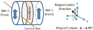
Figure 1: Simplified schematic diagram of an STT-RAM memory element. The nanomagnets (NMs) are on the $y$-$z$ plane and are shaped like elliptical cylinders. NM-1 is magnetically hardened along the $z$-axis so that its magnetization direction is fixed. The magnetization direction of NM-2 can be rotated with an in-plane spin polarized current that delivers a spin-transfer-torque. The magnetization orientation of the free layer NM-2 with respect to the z-axis ($0^{\circ}$ and $180^{\circ}$) encodes logic bits 0 and 1.

It therefore appears that reducing $M_{s}$, while increasing shape anisotropy to keep $E_{b}$ constant, is always beneficial. There is however one caveat. Reducing $M_{s}$ makes a nanomagnet more vulnerable to thermal fluctuations Skumryev et al. (2003) and can increase both the thermally averaged (mean) switching delay and the standard deviation in the switching delay due to thermal fluctuations. This has a deleterious effect on clock speed and clock synchronization in memory or logic technologies utilizing spin-transfer torque mechanism. Consequently, memory and logic devices utilizing materials with low saturation magnetization often work at low temperatures, even if the Curie temperature of the nanomagnet exceeds room temperature, just so that thermal agitations are suppressed Ohno et al. (1996); Mark et al. (2011). In this paper, we show that a better approach to contend with thermal fluctuations, when $M_{s}$ is reduced, is to still work at room temperature, but use slightly more switching current than that required by the $I_{s}\propto M_{s}^{2}$ scaling law. This will decrease the mean switching delay and its variance, while still maintaining a significant energy saving due to the reduced $M_{s}$.

II Model

We study the magnetization dynamics of a nanomagnet subjected to a spin-transfer-torque at room temperature by employing the stochastic Landau-Lifshitz-Gilbert (LLG) equation Landau and Lifshitz (1935); Gilbert (2004). It describes the time evolution of the magnetization vector in the presence of spin-transfer-torque, the torque due to shape anisotropy, and an additional random torque due to thermal fluctuations. We choose the dimensions of the nanomagnet such that it has always a single ferromagnetic domain Cowburn et al. (1999). Thermal effects in magnetization dynamics have been studied both theoretically Fidler and Schrefl (2000); Apalkov and Visscher (2005); Li and Zhang (2004); He, Sun, and Zhang (2007); Wang et al. (2008); Cheng et al. (2006) and experimentally Koch, Katine, and Sun (2004); Myers et al. (2002); Bedau et al. (2010).

We consider a nanomagnet (see Fig. 1) in the shape of an elliptical cylinder whose elliptical cross section lies in the $y$-$z$ plane with its major axis and minor axis aligned along the $z$-direction and the $y$-direction, respectively. The dimension of the major axis is $a$, that of the minor axis is $b$, and the thickness is $l$. The magnet’s volume is $\Omega=(\pi/4)abl$. Let $\theta(t)$ be the angle subtended by the magnetization axis with the +$z$-axis at any instant of time $t$ and $\phi(t)$ be the angle between the +$x$-axis and the projection of the magnetization axis on the $x$-$y$ plane. Thus, $\theta(t)$ is the polar angle and $\phi(t)$ is the azimuthal angle. Note that when $\phi$ = $\pm$ 90^∘, the magnetization vector lies in the plane of the nanomagnet.

The potential energy of an isolated unperturbed shape-anisotropic single-domain nanomagnet is the uniaxial shape anisotropy energy given by

$$E_{SHA}(t)=\frac{\mu_{0}}{2}M_{s}^{2}\Omega N_{d}(t),$$ (1)

where $M_{s}$ is the saturation magnetization and $N_{d}$ is the demagnetization factor expressed as Chikazumi (1964)

$$N_{d}(t)=N_{d-zz}cos^{2}\theta(t)+N_{d-yy}sin^{2}\theta(t)\,sin^{2}\phi(t)\\ +N_{d-xx}sin^{2}\theta(t)\,cos^{2}\phi(t)$$ (2)

with $N_{d-zz}$, $N_{d-yy}$, and $N_{d-xx}$ being the components of $N_{d}$ along the $z$-axis, $y$-axis, and $x$-axis, respectively. The expressions for these quantities can be found in Ref. [Beleggia et al., 2005] and they are constrained by the following relation:

$$N_{d-zz}+N_{d-yy}+N_{d-xx}=1.$$ (3)

We have assumed that the use of a properly balanced synthetic antiferromagnetic fixed layer can eliminate the net effect of dipole coupling on the free layer Liu et al. (2009).

At any instant of time, the total energy of the unperturbed isolated nanomagnet can be expressed as

$$E(t)=E_{SHA}(t)=B(t)sin^{2}\theta(t)+C$$ (4)

where

$$B(t) = B(\phi(t))=\frac{\mu_{0}}{2}\,M_{s}^{2}\Omega\left[N_{d-xx}cos^{2}\phi(t)\right.$$ (5)

$$\qquad\qquad\left.+N_{d-yy}sin^{2}\phi(t)-N_{d-zz}\right],$$

$$C = \frac{\mu_{0}}{2}M_{s}^{2}\Omega N_{d-zz}.$$ (6)

The in-plane shape anisotropy energy barrier height (using $\phi=\pm 90^{\circ}$) can be expressed as

$$E_{SHA,in-plane}=\frac{\mu_{0}}{2}\,M_{s}^{2}\Omega N_{d0}$$ (7)

where $N_{d0}=\left[N_{d-yy}-N_{d-zz}\right]$. Note that the in-plane shape anisotropy energy barrier height is independent of time $t$ even though $E_{SHA}(t)$ is not.

The magnetization M(t) of the single-domain nanomagnet has a constant magnitude at any given temperature but a variable direction, so that we can represent it by the vector of unit norm $\mathbf{n_{m}}(t)=\mathbf{M}(t)/|\mathbf{M}|=\mathbf{\hat{e}_{r}}$ where $\mathbf{\hat{e}_{r}}$ is the unit vector in the radial direction in spherical coordinate system represented by ($r$,$\theta$,$\phi$). The other two unit vectors in the spherical coordinate system are denoted by $\mathbf{\hat{e}_{\theta}}$ and $\mathbf{\hat{e}_{\phi}}$ for $\theta$ and $\phi$ rotations, respectively. The coordinates ($\theta$,$\phi$) completely describe the motion of M(t) Sun (2000).

The torque acting on the magnetization within unit volume due to shape anisotropy is

$$\mathbf{T_{E}}(t) = -\mathbf{n_{m}}(t)\times\nabla\mathbf{E}[\theta(t),\phi(t)]$$

$$= -\{2B(t)sin\theta(t)cos\theta(t)\}\mathbf{\hat{e}_{\phi}}-\{B_{0e}(t)\,sin\theta(t)\}\mathbf{\hat{e}_{\theta}},$$

where

$$B_{0e}(t)=B_{0e}(\phi(t))=\frac{\mu_{0}}{2}\,M_{s}^{2}\Omega(N_{d-xx}-N_{d-yy})sin(2\phi(t)).$$ (9)

Passage of a constant spin-polarized current $I_{s}$ through the nanomagnet generates a spin-transfer-torque that is given by Sun (2000)

$$\mathbf{T_{STT}}(t)=s\,sin\theta(t)\,\mathbf{\hat{e}_{\theta}},$$ (10)

where $s=(\hbar/2e)\eta I_{s}$ is the spin angular momentum deposition per unit time and $\eta$ is the degree of spin-polarization in the current $I_{s}$.

The effect of thermal fluctuations is to produce a random magnetic field $\mathbf{h}(t)$ expressed as

$$\mathbf{h}(t)=h_{x}(t)\,\mathbf{\hat{e}_{x}}+h_{y}(t)\,\mathbf{\hat{e}_{y}}+h_{z}(t)\,\mathbf{\hat{e}_{z}}$$ (11)

where $h_{x}(t)$, $h_{y}(t)$, and $h_{z}(t)$ are the three components in $x$-, $y$-, and $z$-direction, respectively. We will assume the same properties of the random field $\mathbf{h}(t)$ as described in the Ref. [Brown, 1963]. Accordingly, the random thermal field can be expressed as Behin-Aein et al. (2010)

$$h_{i}(t)=\sqrt{\cfrac{2\alpha kT}{|\gamma|(1+\alpha^{2})M_{V}\Delta t}}\;G_{(0,1)}(t)\qquad(i=x,y,z)$$ (12)

where $\alpha$ is the dimensionless phenomenological Gilbert damping constant, $\gamma=2\mu_{B}\mu_{0}/\hbar$ is the gyromagnetic ratio for electrons and is equal to $2.21\times 10^{5}$ (rad.m).(A.s)^-1, $\mu_{B}$ is the Bohr magneton, $M_{V}=\mu_{0}M_{s}\Omega$, $1/\Delta t$ is the attempt frequency of the random thermal field affecting the magnetization dynamics; therefore $\Delta t$ should be chosen as the simulation time-step used to solve the coupled LLG equations numerically, and $G_{(0,1)}(t)$ is a Gaussian distribution with zero mean and unit standard deviation. Note that the variance in the random thermal fields is inversely proportional to the saturation magnetization $M_{s}$; therefore a lower saturation magnetization augments the detrimental effects of thermal fluctuations.

The thermal torque can be written as

$$\mathbf{T_{TH}}(t)=M_{V}\;\mathbf{n_{m}}(t)\times\mathbf{h}(t)=P_{\theta}(t)\,\mathbf{\hat{e}_{\phi}}-P_{\phi}(t)\,\mathbf{\hat{e}_{\theta}}$$ (13)

where

$$P_{\theta}(t)=M_{V}[h_{x}(t)\,cos\theta(t)\,cos\phi(t)+h_{y}(t)\,cos\theta(t)sin\phi(t)\\ -h_{z}(t)\,sin\theta(t)],$$ (14)

$$P_{\phi}(t)=M_{V}[h_{y}(t)\,cos\phi(t)-h_{x}(t)\,sin\phi(t)].$$ (15)

The magnetization dynamics of the single-domain nanomagnet under the action of various torques is described by the stochastic Landau-Lifshitz-Gilbert (LLG) equation as

$$\frac{d\mathbf{n_{m}}(t)}{dt}-\alpha\left(\mathbf{n_{m}}(t)\times\frac{d\mathbf{n_{m}}(t)}{dt}\right)\\ =-\frac{|\gamma|}{M_{V}}\left[\mathbf{T_{E}}(t)+\mathbf{T_{STT}}(t)+\mathbf{T_{TH}}(t)\right].$$ (16)

In spherical coordinate system, with constant magnitude of magnetization, we get the following coupled equations for $\theta$- and $\phi$-dynamics.

$$\left(1+\alpha^{2}\right)\theta^{\prime}(t)=\frac{|\gamma|}{M_{V}}[(B_{0e}(t)-s)sin\theta(t)\\ -2\alpha B(t)sin\theta(t)cos\theta(t)+\left(\alpha P_{\theta}(t)+P_{\phi}(t)\right)]$$ (17)

$$\left(1+\alpha^{2}\right)\phi^{\prime}(t)=\frac{|\gamma|}{M_{V}}[\alpha(B_{0e}(t)-s)\\ +2B(t)cos\theta(t)-[sin\theta(t)]^{-1}\left(P_{\theta}(t)-\alpha P_{\phi}(t)\right)].$$ (18)

The application of an in-plane spin-polarized current $I_{s}$ to produce spin-transfer torque results in an energy dissipation $I_{s}^{2}R\tau$, where $R$ is the in-plane resistance of the elliptical cylinder given by $R=\rho(2/\pi)\,(b/a)\,l$ with $\rho$ being is the resistivity of the material used and $\tau$ is the switching delay.

Furthermore, because of Gilbert damping in the nanomagnet, an additional energy $E_{d}$ is dissipated when the magnetization axis in the nanomagnet switches from one orientation to the other along the easy axis. This energy is given by the expression $E_{d}=\int_{0}^{\tau}P_{d}(t)dt$, where $\tau$ is the switching delay and $P_{d}(t)$ is the dissipated power given by Sun and Wang (2005); Behin-Aein, Salahuddin, and Datta (2009)

$$P_{d}(t)=\frac{\alpha\,|\gamma|}{(1+\alpha^{2})M_{V}}\left|\mathbf{T_{E}}(t)+\mathbf{T_{STT}}(t)\right|^{2}.$$ (19)

Thermal torque does not cause any net energy dissipation since mean of the thermal field is zero.

The thermal distributions of $\theta$ and $\phi$ in an unperturbed magnet are found by solving the Equations (17) and (18) while setting $I_{s}$ = 0. This will yield the distribution of the magnetization vector’s initial orientation ($\theta_{init}$, $\phi_{init}$) when stress is turned on. We consider magnetization intially situates at $\theta=180^{\circ}$. The $\theta$-distribution is Boltzmann peaked at $\theta=180^{\circ}$ with mean $\sim$175.5^∘, while the $\phi$-distribution is Gaussian peaked at $\phi=\pm 90^{\circ}$ sup .

The quantity $\tau$ for any switching trajectory is determined by solving the coupled equations (17) and (18) starting with an initial orientation ($\theta_{init}$, $\phi_{init}$) and terminating the trajectory when $\theta(t)$ reaches a pre-defined $\theta_{final}$, regardless of what the corresponding $\phi_{final}$ is. The time taken for a trajectory to complete (i.e., for $\theta(t)$ to reach $\theta_{final}$) is the value of $\tau$ for that trajectory. The average value $\langle\tau\rangle$ and the standard deviation $\langle\Delta\tau\rangle$ are found by simulating numerous (10,000) trajectories in the presence of the random thermal torque, and then extracting these quantities from the distribution.

The total energy $E_{total}$ dissipated in completing any trajectory is given by $E_{total}=E_{d}+I_{s}^{2}R\tau$. The average power dissipated in completing any trajectory is simply $E_{total}/\tau$. We can find the thermal average of $E_{d}$ and its variance by calculating $E_{d}$ for numerous trajectories and then computing these quantities from the distribution.

III Simulation results

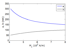
Figure 2: Variation of the major axis ($a$) and the minor axis ($b$) with the saturation magnetization ($M_{s}$) needed to maintain a constant in-plane shape anisotropy barrier of 0.8 eV or $\sim$32 $kT$ at room temperature. The thickness of the nanomagnet is held constant at $l=2$ nm.

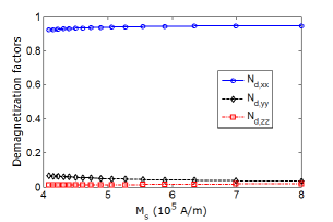
Figure 3: Demagnetization factors needed for different values of saturation magnetization $M_{s}$ in order to keep the in-plane shape anisotropy barrier constant at 0.8 eV or $\sim$32 $kT$ at room temperature. The demagnetization factors are computed from the major and minor axes values in Fig. 2 and with constant thickness of 2 nm.

We consider a nanomagnet made of CoFeB alloy which has low saturation magnetization Yagami et al. (2004) and a low Gilbert damping factor of $\alpha$ = 0.01. The saturation magnetization can be varied by varying the alloy composition Yagami et al. (2004). The resistivity is assumed to be the same as that of cobalt, i.e. $\rho=5.81\times 10^{-8}$ $\Omega$-m [Ref. mat, ]. We choose this material over dilute magnetic semiconductors which have much smaller $M_{s}$ because the latter’s $M_{s}$ is so small Ohno et al. (1996); Mark et al. (2011) that it will be impossible to make the in-plane shape anisotropy barrier $E_{b}$ (which is proportional to $M_{s}^{2}\Omega N_{d0}$) large enough (32 $kT$ or 0.8 eV) without making the volume $\Omega$ of the nanomagnet very large. With that large volume, the nanomagnet will no longer be single-domain. Choosing CoFeB allows us to work at room temperature with a barrier of 0.8 eV or $\sim$32 kT, while still ensuring single-domain behavior because the volume can be kept small.

In order to maintain a constant value of $E_{b}$ = 0.8 eV as we vary $M_{s}$, we increase the shape anisotropy of the nanomagnet (or the aspect ratio $a/b$ of the ellipse) to increase $N_{d0}$ and compensate for any decrease in $M_{s}$. As we vary the aspect ratio $a/b$, we keep the cross-sectional area of the ellipse $[(\pi/4)\,ab]$ and the thickness $l$ constant, which keeps both the area and the volume of the nanomagnet $\Omega$ constant. The rationale behind keeping the cross-sectional area of the nanomagnet constant is to keep the density of devices per unit area on the chip constant.

The in-plane shape anisotropy energy barrier depends on three quantities: $M_{s}$, $N_{d0}$ and $\Omega$ [see Equation (7)]. Since we keep $\Omega$ constant, we compensate for any decrease in $M_{s}$ by commensurately increasing $N_{d0}$ alone. At all times, we ensure that the dimensions chosen ($a$, $b$, and $l$) guarantee that the nanomagnet remains in the single-domain limit Beleggia et al. (2005); Cowburn et al. (1999). The thickness $l$ is held constant at 2 nm.

Fig. 2 shows how the major axis $a$ and the minor axis $b$ should vary with $M_{s}$ to keep the in-plane shape anisotropy energy barrier constant at 0.8 eV. This ensures that the static error probability associated with spontaneous switching between the two stable states along the easy axis remains constant as we vary $M_{s}$ and $N_{d0}$. In Fig. 3, we plot the three components of demagnetization factor for different values of $M_{s}$ that will keep the in-plane shape anisotropy barrier constant at 0.8 eV. Obviously, as $M_{s}$ is decreased, we need to increase the value of $N_{d0}$, i.e. $\left(N_{d-yy}-N_{d-zz}\right)$, to keep the same in-plane shape anisotropy energy barrier height. With decreasing $M_{s}$, the quantity $N_{d-yy}$ increases significantly while $N_{d-zz}$ remains more or less constant. Since the three components of the demagnetization factor are constrained by the relation $N_{d-xx}+N_{d-yy}+N_{d-zz}=1$, the value of $N_{d-xx}$ must decrease proportionately, which is seen in Fig. 3.

III.1 Dependence of switching delay and energy dissipation on saturation magnetization

We assume that when a spin-polarized current is applied to initiate switching, the magnetization vector starts out from near the south pole ($\theta\simeq 180^{\circ}$) with a certain ($\theta_{init}$,$\phi_{init}$) picked from the initial angle distributions at 300 K sup . The magnetization dynamics ensures that $\theta$ continues to rotate towards $0^{\circ}$, while temporary backtracking of $\theta$ may occur due to random thermal kicks. Thermal fluctuations can introduce a spread in the time it takes to reach $\theta\simeq 0^{\circ}$ but cannot prevent magnetization to reach $\theta\simeq 0^{\circ}$. When $\theta$ becomes $\leq 4.5^{\circ}$, switching is deemed to have completed. A moderately large number (10,000) of simulations, with their corresponding ($\theta_{init}$,$\phi_{init}$) picked from the initial angle distributions, are performed for each value of saturation magnetization to generate the simulation results in this subsection. The magnitude of the switching current $I_{s}$ is 2 mA at $M_{s}=8\times 10^{5}$ A/m and it is reduced proportionately with the square of $M_{s}$ for other values of $M_{s}$. The spin polarization of the current is always 80%.

Figs. 4 and 5 show the mean switching delay and the mean energy dissipation for different values of saturation magnetization $M_{s}$ when the in-plane shape anisotropy energy barrier is held constant at 0.8 eV by adjusting the nanomagnet’s shape (and thus demagnetization factors) as we vary $M_{s}$. In generating these plots, the magnitude of the in-plane spin-polarized current is chosen as 2 mA when $M_{s}=8\times 10^{5}$ A/m and the switching current $I_{s}$ was decreased in accordance with the $I_{s}\propto M_{s}^{2}$ scaling law. Each scattered point (denoted ‘single run’) in the figure is the switching delay for one representative switching trajectory at that value of $M_{s}$. There is considerable scatter in the ‘single run’ data which is significantly reduced by thermal averaging (averaging over many trajectories).

The large scatter in the ‘single run’ data points is not caused by the random thermal torque since we get the similar trend without incorporating thermal fluctuations. The scatter is more prominent at smaller values of $M_{s}$, which corresponds to lower $I_{s}$ ($I_{s}\propto M_{s}^{2}$). At lower $I_{s}$, the magnetization dynamics is more complex since there are more ripples (see Fig. 8 and Fig. 9 later). As a result, there is more variability in the switching dynamics (and hence switching delay) with changing $I_{s}$ when the latter is small. This variability contributes to the scatter.

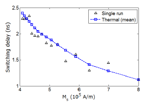
Figure 4: Switching delay $\tau$ at room temperature (300 K) in a nanomagnet of fixed in-plane shape anisotropy energy barrier of 0.8 eV as a function of saturation magnetization $M_{s}$. Switching current $I_{s}$ is 2 mA at $M_{s}=8\times 10^{5}$ A/m and it is reduced proportionately with the square of $M_{s}$ for other values of $M_{s}$. The spin polarization of the current is always 80%.

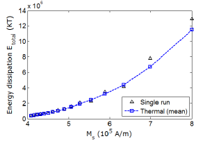
Figure 5: Total energy dissipation in a nanomagnet of fixed in-plane shape anisotropy energy barrier of 0.8 eV as a function of saturation magnetization $M_{s}$ at room temperature (300 K). The total dissipation includes the dissipation in the switching circuit $I_{s}^{2}R\tau$ and the internal energy dissipation $E_{d}$. The internal energy dissipation $E_{d}$ is only a very small fraction of the total energy dissipation $E_{total}$.

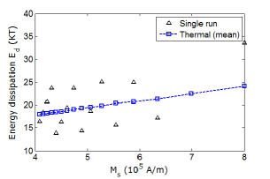
Figure 6: Internal energy dissipation $E_{d}$ for different values of saturation magnetization at 300 K. This energy dissipation is several orders of magnitude smaller than the energy dissipation in the external circuitry thus it is only a very small fraction of the total energy dissipation $E_{total}$.

In Fig. 4, we find that the mean switching delay $\langle\tau\rangle$ decreases with increasing saturation magnetization $M_{s}$. This can be explained as follows. The spin-transfer torque is proportional to $I_{s}$/$M_{s}$. Since $I_{s}\propto M_{s}^{2}$, the spin-transfer-torque becomes proportional to $M_{s}$. Therefore, reducing $M_{s}$ weakens the spin-transfer-torque. Since the in-plane shape anisotropy energy barrier is invariant, it takes longer for the weakened spin-transfer torque to overcome the in-plane shape anisotropy barrier and cause switching. This makes switching delay increase with decreasing $M_{s}$.

In Fig. 5, we plot the thermal means of the energy dissipation $E_{total}$ at 300 K as a function of the saturation magnetization $M_{s}$, while keeping the in-plane shape anisotropy barrier constant. $E_{total}$ is overwhelmingly dominated by the component $I_{s}^{2}R\tau$, and the internal energy dissipation $E_{d}$ has a minor contribution [see Fig. 6]. The switching current $I_{s}$ varies as the square of $M_{s}$, so that $I_{s}^{2}$ varies as $M_{s}^{4}$. Furthermore, if we reduce $M_{s}$, we have to increase the shape anisotropy (or the aspect ratio $a/b$) to keep the in-plane shape anisotropy energy barrier constant. If the switching current flows along the minor axis of the elliptical nanomagnet (always preferable since it results in minimum resistance in the path of the current), then increasing the ratio $a/b$ decreases the nanomagnet’s electrical resistance proportionately. Thus, both $I_{s}$ and $R$ will decrease with decreasing $M_{s}$ (the latter because the in-plane shape anisotropy barrier is kept constant). Consequently, the power dissipation $I_{s}^{2}R$ increases with $M_{s}$ more rapidly than $M_{s}^{4}$. Unless the switching delay $\tau$ has a stronger dependence on $M_{s}$ than $\tau\propto M_{s}^{-4}$, we will expect the energy dissipation to decrease with decreasing $M_{s}$ and that is precisely what we observe in Fig. 5.

The last two figures highlight two important facts: (1) the energy dissipated to switch can be reduced by decreasing $M_{s}$ while maintaining a fixed in-plane shape anisotropy energy barrier to keep the static error probability fixed, and (2) the switching delay increases if we reduce $M_{s}$ while keeping the in-plane shape anisotropy energy barrier fixed. Thus, there are two penalties involved with reducing energy dissipation by lowering $M_{s}$ and scaling $I_{s}$ quadratically with $M_{s}$: (i) slower switching, and (ii) higher dynamic error probability due to an increased variance in thermal field [see Equation (12)].

For the nanomagnet that we have considered (with the parameters described earlier), we find that lowering the saturation magnetization $M_{s}$ by a factor of $\sim$2 decreases the energy dissipation by $\sim$28 times while increasing the switching delay by approximately twice. The factor of $\sim$2 decrease in $M_{s}$ causes a $\sim$16-fold decrease in $I_{s}^{2}$ (since $I_{s}\propto M_{s}^{2}$). Additionally, there is $\sim$4-fold decrease in the resistance of the nanomagnet owing to the fact that the shape anisotropy is increased to keep the in-plane shape anisotropy energy barrier constant. Thus, the $\sim$64-fold decrease in power dissipation and the 2-fold increase in switching delay together cause a net decrease of $\sim$28 times in the total energy dissipation. Therefore, if we decrease the saturation magnetization by a factor of $\sim$2, then we will: (1) gain 28-fold in energy dissipation; (2) lose 2-fold in switching speed; and (3) lose somewhat in error rates due to thermal agitation since the variance in switching delay is increased.

III.2 Constant switching delay scaling

In order to understand how we can maintain a constant switching delay while scaling $M_{s}$, let us consider the relationship between switching current and switching delay. In Figs. 7 and 8, we plot the magnetization dynamics without considering any thermal fluctuations during the switching when $M_{s}=8\times 10^{5}$ A/m and $M_{s}=4.09\times 10^{5}$ A/m, respectively. The switching current has been decreased from 2 mA for $M_{s}=8\times 10^{5}$ A/m to 523 $\mu$A for $M_{s}=4.09\times 10^{5}$ A/m, in accordance with the square-law scaling $I_{s}\propto M_{s}^{2}$. In Figs. 7 and 8, we have assumed the same initial orientation of magnetization $\theta_{init}=175.5^{\circ}$ and $\phi_{init}=90^{\circ}$, which are thermally mean values for 300 K to avoid the stagnation point exactly along the easy axis. The square-law scaling however results in an increased switching delay since the latter has obviously increased by a factor of 2 (from 1.05 ns to 2.1 ns). This has happened because of more ripples generating from more precessional motion of the magnetization vector seen in Fig. 8. In order to maintain the same switching delay of 1.05 ns as before, we will have to deviate from the square-law scaling and increase the switching current by nearly two times to 1.05 mA. Thus, we need to pump an excess current of 1.05 mA - 0.523 mA = 0.527 mA in order to maintain the same switching speed. The corresponding magnetization dynamics without considering any thermal fluctuations during the switching is shown in Fig. 9, where we have clearly recovered the 1.05 ns delay. The energy dissipation (dominated by $I_{s}^{2}R\tau$) now goes up by a factor of two [$I_{s}$ increases by a factor of two while $\tau$ decreases by a factor of two]. Thus, we find that if we wish to maintain a constant switching delay, then we need to inject some excess current over that dictated by square-law scaling and therefore suffer some excess energy dissipation. This excess energy dissipation is sufficiently small so that there is still considerable energy saving accruing from the reduction in $M_{s}$. Reducing $M_{s}$ by a factor of $\sim$2 results in a net energy saving of $\sim$14 times, instead of the $\sim$28 times estimated without imposing the requirement of constant switching delay. The important point is that we have extracted a very significant energy saving by reducing $M_{s}$ by a factor of 2, without sacrificing switching speed.

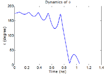
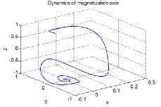
Figure 7: Switching dynamics of the magnetization vector in a nanomagnet of major axis $a$ = 150 nm, minor axis $b$ = 100 nm, and $M_{s}=8\times 10^{5}$ A/m, and in-plane shape anisotropy energy barrier of 0.8 eV. This simulation does not consider any thermal fluctuations during the switching, however, the initial orientation of the magnetization is assumed to be $\theta_{init}=175.5^{\circ}$ and $\phi_{init}=90^{\circ}$ (thermally mean values for 300 K) to avoid the stagnation point exactly along the easy axis. Switching is caused by spin-transfer torque induced with an in-plane current of 2 mA with 80% spin polarization. (a) polar angle $\theta(t)$ versus time, and (b) the trajectory traced out by the tip of the magnetization vector during switching. Switching delay and energy dissipation are 1.05 ns and $1.25\times 10^{7}$ $kT$ [at room temperature], respectively.

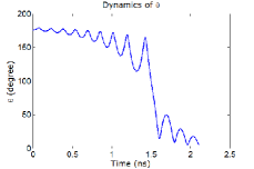
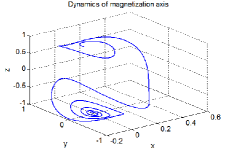
Figure 8: Switching dynamics for $M_{s}=4.09\times 10^{5}$ A/m and spin-transfer torque switching current $I_{s}$ of 523 $\mu$A with 80% spin polarization. This simulation does not consider any thermal fluctuations during the switching, however, the initial orientation of the magnetization is assumed to be $\theta_{init}=175.5^{\circ}$ and $\phi_{init}=90^{\circ}$ (thermally mean values for 300 K) to avoid the stagnation point exactly along the easy axis. (a) Polar angle $\theta(t)$ versus time, and (b) the trajectory traced out by the tip of the magnetization vector while switching occurs. The switching delay and the energy dissipation are 2.1 ns and $4.3\times 10^{5}$ $kT$ [at room temperature], respectively.

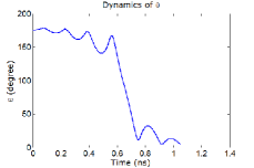
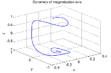
Figure 9: Switching dynamics for $M_{s}=4.09\times 10^{5}$ A/m and spin-transfer torque switching current $I_{s}$ of 1.05 mA with 80% spin polarization. This simulation does not consider any thermal fluctuations during the switching, however, the initial orientation of the magnetization is assumed to be $\theta_{init}=175.5^{\circ}$ and $\phi_{init}=90^{\circ}$ (thermally mean values for 300 K) to avoid the stagnation point exactly along the easy axis. (a) Polar angle $\theta(t)$ versus time, and (b) the trajectory traced out by the tip of the magnetization vector while switching occurs. The switching delay and the energy dissipation are 1.05 ns and $8.6\times 10^{5}$ $kT$ [at room temperature], respectively.

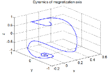
Figure 10: Switching dynamics at 300 K for $M_{s}=4.09\times 10^{5}$ A/m and spin-transfer torque switching current $I_{s}$ of 1.05 mA with 80% spin polarization. The initial orientation of the magnetization is $\theta_{init}=175.5^{\circ}$ and $\phi_{init}=90^{\circ}$, which are the thermal mean values. This is one specific run from 10,000 MC simulations. (a) Polar angle $\theta(t)$ versus time, and (b) the trajectory traced out by the tip of the magnetization vector while switching occurs. The switching delay and the energy dissipation are 1.18 ns and $9.6\times 10^{5}$ $kT$ [at room temperature], respectively.

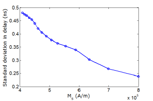
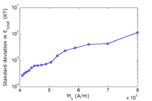
Figure 11: Standard deviation in switching delay and energy dissipation due to thermal fluctuations at 300 K as a function of saturation magnetization $M_{s}$ in a nanomagnet with fixed in-plane shape anisotropy energy barrier of 0.8 eV. (a) Standard deviation in switching delay. (b) Standard deviation in energy dissipation.

For illustrative purposes, we show in Fig. 10 the magnetization dynamics in the presence of thermal fluctuations at 300 K for the same parameters as in Fig. 9. This is one representative run picked out from 10,000 simulations of the switching trajectory. Note that there is only some quantitative difference, but not much qualitative difference, between Figs. 9 and 10. The ripples are somewhat larger in amplitude and the precessional motion is slightly exacerbated. The switching delay has increased by $\sim$12% in the presence of thermal agitations, however, it should be pointed out that the switching delay may decrease as well when the net effect of thermal agitations aids the magnetization rotation.

Fig. 11 shows how the standard deviations in switching delay and energy dissipation due to thermal fluctuations depend on the saturation magnetization $M_{s}$. As expected, the standard deviation in switching delay increases with decreasing $M_{s}$, because the random thermal fields $h_{i}(t)$ (i=$x$,$y$,$z$), which are responsible for the standard deviation, has a $1/\sqrt{M_{s}}$ dependence [see Equation (12)]. Furthermore, if we scale $I_{s}$ as $M_{s}^{2}$, then the spin-transfer torque also decreases as we reduce $M_{s}$ and that makes the increased thermal field even more effective in randomizing the switching delay. For this reason, the error probability (or switching failure rate) increases when $M_{s}$ decreases. This problem too can be overcome with some excess switching current. Our simulations have shown that if we increase the switching current from 523 $\mu$A to 1.05 mA, while holding $M_{s}$ constant at 4.09$\times$10⁵ A/m, then the standard deviation in the switching delay goes down from 0.48 ns to 0.23 ns. Note that in this way we have recovered approximately the same standard deviation in switching delay as that for $M_{s}=8\times$10⁵ A/m.

The standard deviation in energy dissipation however shows the opposite trend, i.e. it decreases with decreasing $M_{s}$. This happens because the energy dissipation $E_{total}$ is dominated by $I_{s}^{2}R\tau$, which is proportional to $M_{s}^{4}R\tau$. Lowering $M_{s}$ increases the standard deviation in $\tau$, but that increase is more than offset by the lower value of $M_{s}$, so that the net standard deviation in $I_{s}^{2}R\tau$ actually decreases with decreasing $M_{s}$. The excess current that we pump now has a deleterious effect. If we increase the switching current from 523 $\mu$A to 1.05 mA while holding $M_{s}$ constant at 4.09$\times$10⁴ A/m, then the standard deviation in energy dissipation goes up from 2.6$\times$10⁴ kT to 9.2$\times$10⁴ kT.

The ratio of the standard deviation to the mean is relatively independent of $M_{s}$ for both the switching delay and the total energy dissipation at 300 K. This ratio does not vary by more than 5% when $M_{s}$ is varied between 4.09$\times$10⁵ and 8$\times$10⁵ A/m.

IV Discussions and conclusions

We have shown that one can significantly reduce energy dissipation in spin-transfer torque driven switching of shape-anisotropic nanomagnets by reducing the saturation magnetization of the magnet with appropriate material choice, while maintaining a constant in-plane shape anisotropy energy barrier (by increasing the magnet’s aspect ratio) and a constant mean switching speed (by pumping some excess current) in the presence of thermal fluctuations. Also, the increased variance in switching delay due to lower saturation magnetization can be mitigated by pumping some excess current. In the end, by employing these strategies, one can make the energy dissipation in spin-transfer torque driven switching of nanomagnets competitive with other technologies, without sacrificing switching speed. This bodes well for applications of spin-transfer torque switched nanomagnets in non-volatile logic and memory.

References

- Slonczewski (1996) J. C. Slonczewski, J. Magn. Magn. Mater. 159, L1 (1996).
- Berger (1996) L. Berger, Phys. Rev. B 54, 9353 (1996).
- Sun (2000) J. Z. Sun, Phys. Rev. B 62, 570 (2000).
- Sun (2006) J. Z. Sun, IBM J. Res. Dev. 50, 81 (2006).
- Gallagher and Parkin (2006) W. J. Gallagher and S. S. P. Parkin, IBM J. Res. Dev. 50, 5 (2006).
- Katine et al. (2000) J. A. Katine, F. J. Albert, R. A. Buhrman, E. B. Myers, and D. C. Ralph, Phys. Rev. Lett. 84, 3149 (2000).
- Fuchs et al. (2006) G. D. Fuchs, J. A. Katine, S. I. Kiselev, D. Mauri, K. S. Wooley, D. C. Ralph, and R. A. Buhrman, Phys. Rev. Lett. 96, 186603 (2006).
- Parkin et al. (1999) S. S. P. Parkin, K. P. Roche, M. G. Samant, P. M. Rice, R. B. Beyers, R. E. Scheuerlein, E. J. O’Sullivan, S. L. Brown, J. Bucchigano, and D. W. Abraham, J. Appl. Phys. 85, 5828 (1999).
- Chappert, Fert, and Dau (2007) C. Chappert, A. Fert, and F. N. V. Dau, Nature Mater. 6, 813 (2007).
- Roy, Bandyopadhyay, and Atulasimha (2011) K. Roy, S. Bandyopadhyay, and J. Atulasimha, Appl. Phys. Lett. 99, 063108 (2011).
- Myers et al. (1999) E. B. Myers, D. C. Ralph, J. A. Katine, R. N. Louie, and R. A. Buhrman, Science 285, 867 (1999).
- Yagami et al. (2004) K. Yagami, A. A. Tulapurkar, A. Fukushima, and Y. Suzuki, Appl. Phys. Lett. 85, 5634 (2004).
- Kubota et al. (2009) H. Kubota, A. Fukushima, K. Yakushiji, S. Yakata, S. Yuasa, K. Ando, M. Ogane, Y. Ando, and T. Miyazaki, J. Appl. Phys. 105, 07D117 (2009).
- Landauer and Swanson (1961) R. Landauer and J. A. Swanson, Phys. Rev. 121, 1668 (1961).
- Landauer (1961) R. Landauer, IBM J. Res. Dev. 5, 183 (1961).
- Likharev (1982) K. K. Likharev, Int. J. Theor. Phys. 21, 311 (1982).
- Skumryev et al. (2003) V. Skumryev, S. Stoyanov, Y. Zhang, G. Hadjipanayis, D. Givord, and J. Nogués, Nature 423, 850 (2003).
- Ohno et al. (1996) H. Ohno, A. Shen, F. Matsukura, A. Oiwa, A. Endo, S. Katsumoto, and Y. Iye, Appl. Phys. Lett. 69, 363 (1996).
- Mark et al. (2011) S. Mark, P. Durrenfeld, K. Pappert, L. Ebel, K. Brunner, C. Gould, and L. W. Molenkamp, Phys. Rev. Lett. 106, 57204 (2011).
- Landau and Lifshitz (1935) L. Landau and E. Lifshitz, Phys. Z. Sowjet. 8, 101 (1935).
- Gilbert (2004) T. L. Gilbert, IEEE Trans. Magn. 40, 3443 (2004).
- Cowburn et al. (1999) R. P. Cowburn, D. K. Koltsov, A. O. Adeyeye, M. E. Welland, and D. M. Tricker, Phys. Rev. Lett. 83, 1042 (1999).
- Fidler and Schrefl (2000) J. Fidler and T. Schrefl, J. Phys. D: Appl. Phys. 33, R135 (2000).
- Apalkov and Visscher (2005) D. M. Apalkov and P. B. Visscher, Phys. Rev. B 72, 180405 (2005).
- Li and Zhang (2004) Z. Li and S. Zhang, Phys. Rev. B 69, 134416 (2004).
- He, Sun, and Zhang (2007) J. He, J. Z. Sun, and S. Zhang, J. Appl. Phys. 101, 09A501 (2007).
- Wang et al. (2008) X. Wang, Y. Zheng, H. Xi, and D. Dimitrov, J. Appl. Phys. 103, 034507 (2008).
- Cheng et al. (2006) X. Z. Cheng, M. B. A. Jalil, H. K. Lee, and Y. Okabe, Phys. Rev. Lett. 96, 67208 (2006).
- Koch, Katine, and Sun (2004) R. H. Koch, J. A. Katine, and J. Z. Sun, Phys. Rev. Lett. 92, 88302 (2004).
- Myers et al. (2002) E. B. Myers, F. J. Albert, J. C. Sankey, E. Bonet, R. A. Buhrman, and D. C. Ralph, Phys. Rev. Lett. 89, 196801 (2002).
- Bedau et al. (2010) D. Bedau, H. Liu, J. Z. Sun, J. A. Katine, E. E. Fullerton, S. Mangin, and A. D. Kent, Appl. Phys. Lett. 97, 262502 (2010).
- Chikazumi (1964) S. Chikazumi, Physics of Magnetism (Wiley New York, 1964).
- Beleggia et al. (2005) M. Beleggia, M. D. Graef, Y. T. Millev, D. A. Goode, and G. E. Rowlands, J. Phys. D: Appl. Phys. 38, 3333 (2005).
- Liu et al. (2009) L. Liu, T. Moriyama, D. C. Ralph, and R. A. Buhrman, Appl. Phys. Lett. 94, 122508 (2009).
- Brown (1963) W. F. Brown, Phys. Rev. 130, 1677 (1963).
- Behin-Aein et al. (2010) B. Behin-Aein, D. Datta, S. Salahuddin, and S. Datta, Nature Nanotechnol. 5, 266 (2010).
- Sun and Wang (2005) Z. Z. Sun and X. R. Wang, Phys. Rev. B 71, 174430 (2005).
- Behin-Aein, Salahuddin, and Datta (2009) B. Behin-Aein, S. Salahuddin, and S. Datta, IEEE Trans. Nanotech. 8, 505 (2009).
- (39) See supplementary material at ……………… for detailed derivations and additional simulation results .
- (40) http://www.allmeasures.com/Formulae/static/materials/.