Understanding the Random Displacement Model:
From Ground-State Properties to Localization

Abstract

We give a detailed survey of results obtained in the most recent half decade which led to a deeper understanding of the random displacement model, a model of a random Schrödinger operator which describes the quantum mechanics of an electron in a structurally disordered medium. These results started by identifying configurations which characterize minimal energy, then led to Lifshitz tail bounds on the integrated density of states as well as a Wegner estimate near the spectral minimum, which ultimately resulted in a proof of spectral and dynamical localization at low energy for the multi-dimensional random displacement model.

1. Introduction

By the random displacement model (RDM) we refer to a random Schrödinger operator of the type

$$H_{\omega}=-\Delta+V_{\omega},\quad V_{\omega}(x):=\sum_{n\in{\mathord{\mathbb{Z}}}^{d}}q(x-n-\omega_{n})$$ (1)

in $L^{2}({\mathord{\mathbb{R}}}^{d})$, $d\geq 1$. The potential is generated by randomly displacing translates of the single-site potential $q$ from the lattice sites $n\in{\mathord{\mathbb{Z}}}^{d}$. More detailed assumptions on $q$ and the random displacements $\omega_{n}$ will be introduced below as needed.

The RDM has proven to be much harder to analyze mathematically than the (continuum) Anderson model

$$H_{\lambda(\omega)}^{A}=-\Delta+\sum_{n\in{\mathord{\mathbb{Z}}}^{d}}\lambda_{n}q(x-n)$$ (2)

with random coupling constants $\lambda_{n}=\lambda_{n}(\omega)$. A fundamental technical difference between the RDM and the Anderson model lies in their monotonicity properties. If the single-site potential $q$ is sign-definite, then the Anderson model is monotone in the random variables $\lambda_{n}$ in quadratic form sense. This is not true for the RDM, independent of sign-assumptions on $q$.

Many of the rigorous tools which have been developed to study the Anderson model rely on its monotonicity properties. In particular, this is true for most of the proofs of localization for the Anderson model near the bottom of its spectrum. In fact, if one considers the Anderson model with sign-indefinite single-site potential $q$, and thus looses monotonicity, then localization results are much more recent and far less complete than for the case of sign-definite $q$, e.g. [40, 32, 24, 34, 35]. The difficulties which arise are in many ways similar to the problems encountered in the RDM. Related phenomena and difficulties also arise in discrete alloy-type models with sign-indefinite single site potential, as recently reviewed in [14].

Among models for continuum random Schrödinger operators, the structural disorder described by the RDM can be considered as physically equally natural as the coupling constant disorder in the Anderson model. Another natural model for structural disorder is the Poisson model

$$-\Delta+\sum_{i}q(x-X_{i}),$$ (3)

with $X_{i}$ denoting the points of a $d$-dimensional Poisson process. The RDM as well as the Poisson model were introduced early on in the mathematical literature on continuum random Schrödinger operators, e.g. [26, 36] and references therein. However, progress has been much more limited than for the Anderson model due to the technical difficulties which arise.

An exception is the case $d=1$, where localization throughout the entire spectrum has been proven for the RDM and the Poisson model in [39, 8, 13]. This was possible based on the powerful dynamical systems methods available to study one-dimensional random operators, in particular those allowing to prove positivity of Lyapunov exponents and to deduce localization from this. However, the non-monotonicity of the RDM and the Poisson model has visible consequences already in the one-dimensional case, for example through the appearance of critical energies in the spectrum at which the Lyapunov exponent vanishes and, in some cases, weaker results (e.g. on dynamical localization, which has not been shown for the one-dimensional Poisson model).

In dimension $d\geq 2$ it is generally expected that “typical” random Schrödinger operators have a localized region at the bottom of the spectrum, at least if the latter corresponds to a fluctuation boundary of the spectrum, which describes a boundary characterized by rare events. The history of localization proofs for the multi-dimensional RDM and Poisson model is told very quickly. For the Poisson model in $d\geq 2$ localization at the bottom of the spectrum was finally proven in [18] for positive single-site potentials and in [19] for negative single-site potentials. In both cases the powerful extension of multi-scale analysis developed by Bourgain and Kenig in [6] was used as a tool.

There were two previous results on localization for the multi-dimensional RDM, [31] and [22]. In [31] a semiclassical version of (1) is considered and localization near the bottom of the spectrum is established for sufficiently small values of a semiclassical coupling parameter at the Laplacian. [22] considers the RDM with an additional periodic term $V_{per}$ and establishes localization for generic (but non-zero) choices of $V_{per}$. In both works the values of the displacements $\omega_{n}$ have to be sufficiently small and first order perturbation effects (such as a monotonicity property of Floquet eigenvalues of $-\Delta+V_{per}$ in [22]) are exploited. What makes the “naked RDM” (1) more difficult to handle is that, as will be pointed out below, one ultimately has to resort to second-order perturbation effects.

The goal of this work is to give a detailed survey of new results for the RDM (1) obtained in the papers [4, 5, 35] and [30], which allowed to understand that the spectral minimum of the RDM is a fluctuation boundary under a natural set of assumptions not requiring additional parameters or smallness of the displacements (other than a non-overlap condition), and ultimately led to a proof of localization in this setting in [30].

The strategy used to prove localization in these works is the one provided by the Fröhlich-Spencer multi-scale analysis [17], as described for continuum models in very accessible form in the book [38], and with state-of-the-art results shown in [20] and surveyed in [29]. In essence, the MSA approach shows that localization, spectral as well as dynamical, can be proven once a smallness result (“Lifshitz tails”) for the integrated density of states at the bottom of the spectrum and a Wegner estimate are available as input.

Therefore much of our effort is aimed at proving these two ingredients. However, for the RDM (1) one first needs to address a preliminary problem: Which configurations $\omega=(\omega_{n})$ characterize the minimum of the almost sure spectrum of $H_{\omega}$? To explain that this is a non-trivial issue, let us compare with the Anderson and Poisson models. In the Anderson model (2), due to monotonicity, the spectrum is minimized by choosing all coupling constants $\lambda_{n}$ minimal (in the support of their distribution) if $q$ is positive, while all $\lambda_{n}$ should be chosen maximal if $q$ is negative. For the Poisson model (3) the spectral minimum is $0$ if $q$ is positive, corresponding to regions with widely separated Poisson points. If $q$ is negative, then regions of densely clustered Poisson points lead to spectral minimum $-\infty$. The mechanism for generating the spectral minimum in the RDM is much less apparent (with similar difficulties arising for the Anderson model with non sign-definite single-site potential). In fact, while for the (definite) Anderson and Poisson model the spectrum is minimized by minimizing the potential, for the RDM we will see that a much more subtle interaction between kinetic and potential energy determines the spectral minimum.

In terms of assumptions to be made, the most important one is that the single-site potential shares the symmetries of the underlying lattice, here ${\mathord{\mathbb{Z}}}^{d}$. It is fair to say that in our approach symmetry replaces the lack of any apparent monotonicity properties of the model, ultimately allowing to identify more delicate monotonicity properties which are at the core of our proofs of Lifshitz tail bounds and a Wegner estimate for the RDM.

We find it remarkable how many mathematical ideas and tools had to be invoked and how all this ultimately fit together quite perfectly to lead to a localization proof for the RDM (1). Getting this across to the reader is our main motivation for providing this expository account of our work. Beyond merely stating a series of results, we include frequent discussions of the underlying motivations, often going beyond what we have been able to include in our previously published work. We have also tried to include at least outlines of all proofs, even if we frequently have to refer to the original papers for additional details.

A rough outline of the contents of the remaining sections of this paper is as follows: In Section 2 we reveal how the spectral minimum of the RDM is found. In Section 3 we show how the proof of this is reduced to a spectral minimization property of a related single-site Neumann operator. This operator and its ground state properties are central to almost all our results. In particular, we will revisit this operator in Section 6 and explain why we ultimately needed to know more about it than what is stated in Section 3. To avoid having to interrupt the telling of our localization story, we outline the proofs of these results in Section 10 near the end of the paper.

The rest of the localization story is told in Sections 4, 5, 7, 8 and 9. Section 4 yields information on uniqueness of configurations characterizing the spectral minimum which is necessary for the proof of Lifshitz tail bounds in Sections 5 and 7. The results in the latter two sections work in form of a boot-strap, starting with a Lifshitz tail bound under strong additional assumptions which are then relaxed. Our Wegner estimate for the RDM is presented in Section 8. In Section 9 we state the exact form of our result on localization for the RDM and provide references to the literature on multi-scale analysis, which show how this is proven based on the Lifshitz tail and Wegner bounds. In the very last Section 11 we discuss some open problems related to our work.

Acknowledgments: G. S. would like to thank the organizers of the conference “Spectral Days”, held in Santiago from September 20 to 24, 2010, for the opportunity to give a lecture series on the work discussed here.

2. The Spectral Minimum of the RDM

We will always assume that the displacement parameters $\omega=(\omega_{n})_{n\in{\mathord{\mathbb{Z}}}^{d}}$ are independent, identically distributed ${\mathord{\mathbb{R}}}^{d}$-valued random variables. Their common distribution is a Borel probability measure on ${\mathord{\mathbb{R}}}^{d}$. As usual, we define its support by

$$\mbox{supp}\,\mu:=\{a\in{\mathord{\mathbb{R}}}^{d}:\mu(B_{\varepsilon}(a))>0\;\mbox{for all}\;\varepsilon>0\},$$

which is a closed set. The i.i.d. random variables $\omega_{n}$ can be realized as the canonical projections $\omega\mapsto\omega_{n}$ in the infinite product probability space

$$(\Omega,{\mathord{\mathbb{P}}})=\left(\otimes_{n\in{\mathord{\mathbb{Z}}}^{d}}{\mathord{\mathbb{R}}}^{d},\otimes_{n\in{\mathord{\mathbb{Z}}}^{d}}\mu\right).$$

Under weak assumptions on $\mu$ and the single-site potential $q$ the RDM $H_{\omega}$ is self-adjoint on the second order Sobolev space in $L^{2}({\mathord{\mathbb{R}}}^{d})$ and ergodic with respect to shifts in ${\mathord{\mathbb{Z}}}^{d}$ in the sense of, e.g., [10]. Thus its spectrum is almost surely deterministic: There exists $\Sigma\subset{\mathord{\mathbb{R}}}$ such that

$$\sigma(H_{\omega})=\Sigma\quad\mbox{for ${\mathord{\mathbb{P}}}$-almost every $\omega$}.$$ (4)

In fact, one has

$$\Sigma=\overline{\bigcup_{\omega\in{\mathcal{C}}_{per}}\sigma(H_{\omega})},$$ (5)

where

$${\mathcal{C}}_{per}:=\{\omega\in{\mathord{\mathbb{Z}}}^{d}\to\;\mbox{supp}\,\mu\>\mbox{periodic with respect to a sub-lattice of}\>{\mathord{\mathbb{Z}}}^{d}\}.$$ (6)

This follows by the same methods which have been used to prove a corresponding result for the Anderson model: That $\Sigma$ is contained in the right hand side of (5) follows by approximating any given random configuration with periodic configurations, truncating the random configuration to large cubes and periodically extending from there. On the other hand, one can show that almost every random configuration comes arbitrarily close to any given periodic configuration on arbitrarily large cubes, which is he idea behind the reverse inclusion. For a detailed proof, written for the case of the Anderson model, we refer to [26].

In particular, (5) implies that

$$E_{0}:=\min\Sigma=\inf\{\min\,\sigma(H_{\omega}):\omega\in{\mathcal{C}}_{per}\}.$$ (7)

It is a non-trivial question to decide if there is a periodic minimizer, i.e. if the infimum in (7) is a minimum. In fact, we do not believe that this is true in general. Our choice of the following assumptions on $q$ and $\mu$ is mostly motivated by the fact that they allow to find a periodic minimizer for (7).

(A1) The single-site potential $q:{\mathord{\mathbb{R}}}^{d}\to{\mathord{\mathbb{R}}}$ is bounded, measurable and reflection-symmetric in each variable. Moreover, supp$\,q\subset[-r,r]^{d}$ for some $r<1/2$.

(A2) Let $d_{max}:=\frac{1}{2}-r$ and ${\mathcal{C}}:=\{(\pm d_{max},\ldots,\pm d_{max})\}$ denote the $2^{d}$ corners of the closure $\overline{G}$ of $G:=(-d_{max},d_{max})^{d}$. Then

$${\mathcal{C}}\subset\>\mbox{supp}\,\mu\subset\overline{G}.$$

The two support assumptions on $q$ and $\mu$ have a simple geometric interpretation for the RDM (1): The support of each single-site term $q(\cdot-n-\omega_{n})$ stays in the unit cell centered at $n$, while it is allowed to “touch” the boundary of the cell. In fact, with positive probability the single-site potentials may move arbitrarily close to each corner of their cell. For a typical configuration of the $\omega_{n}$ see Figure 1 (where the support of $q$ is drawn radially symmetric for aesthetic reasons).

Figure 1. The support of $V_{\omega}$ for a typical $\omega$.

We can now identify a periodic minimizer for (7), stating a result from [4]:

Theorem 2.1.

Assume (A1) and (A2) and let $\omega^{*}=(\omega_{n}^{*})_{n\in{\mathord{\mathbb{Z}}}^{d}}$ be given by

$$\omega_{n}^{*}:=((-1)^{n_{1}}d_{max},\ldots,(-1)^{n_{d}}d_{max}),\quad n=(n_{1},\ldots,n_{d})\in{\mathord{\mathbb{Z}}}^{d}.$$ (8)

Then $E_{0}=\min\sigma(H_{\omega^{*}})$.

The potential $V_{\omega^{*}}(x)=\sum_{n}q(x-n-\omega_{n}^{*})$ is 2-periodic in each direction and locally consists of densest clusters of $2^{d}$ single-site terms placed into adjacent corners of their cells, see Figure 2.

Figure 2. Support of $V_{\omega^{*}}$ for $d=2$.

One may understand this result heuristically by the following strategy to construct test-functions which minimize the quadratic form of $H_{\omega}$, at least if the single-site potential $q$ is negative: The clusters in $V_{\omega^{*}}$ form wide wells. In these wells one can place localized test functions with relatively small derivative, due to the width of the wells, i.e. small cost in kinetic energy. This gives lower total energy than the narrower wells given by individual, spatially separated single-site potentials. This is not how Theorem 2.1 is proven. We should also point out that Theorem 2.1 does not impose any sign-restrictions on $q$, and thus can not be fully explained by the above heuristics. But the heuristics make clear that the spectral minimum of the RDM is determined by a non-trivial interplay between kinetic and potential energy.

Instead we will give a proof of Theorem 2.1 at the end of the next section, based on the answer to a minimization problem for a single-site Neumann operator associated with the RDM.

3. The Neumann Problem

Theorem 2.1 provides the answer to an optimization problem involving infinitely many displacement parameters $\omega_{n}$, $n\in{\mathord{\mathbb{Z}}}^{d}$. However, due to the symmetry assumptions on $q$, it turns out that the proof can be reduced to a related problem involving the optimal placement of just one single-site term.

For this purpose, let $\Lambda_{1}:=(-\frac{1}{2},\frac{1}{2})^{d}$ be the unit cube centered at the origin and $-\Delta^{N}$ the Neumann-Laplacian on $L^{2}(\Lambda_{1})$, i.e. the unique self-adjoint operator whose quadratic form is $\int_{\Lambda_{1}}|\nabla f(x)|^{2}\,dx$ for $f\in H^{1}(\Lambda_{1})$, the first order Sobolev space.

For $q$ as in (A1) and $a\in\overline{G}$ let

$$H_{\Lambda_{1}}^{N}(a):=-\Delta^{N}+q(x-a)$$

and $E_{0}(a):=\min\sigma(H_{\Lambda_{1}}^{N}(a))$ the non-degenerate lowest eigenvalue of $H^{N}_{\Lambda_{1}}(a)$. For a general discussion of properties of operators of this type see Section 2 of [4].

We ask for the optimal placement of $a\in\overline{G}$ to minimize $E_{0}(a)$ and arrive at the following result.

Theorem 3.1.

Under assumption (A1) one of the following two alternatives holds:

(i) $E_{0}(a)$ is strictly maximized at $a=0$ and strictly minimized at the corners ${\mathcal{C}}$ of $\overline{G}$.

(ii) $E_{0}(a)$ is identically zero.

A proof of Theorem 3.1 under the given assumptions can be found in [4]. We will not discuss details of this proof here, as we will later need a strengthened version of Theorem 3.1 for which we will also use somewhat stronger assumptions, see Theorem 6.1 and assumption (A1)’ in Section 6 below.

The proof of Theorem 3.1 in [4] shows that in each of the two alternatives more can be said:

In case of alternative (i), the function $E_{0}(a_{1},\ldots,a_{j},\ldots,a_{d})$ is symmetric and strictly unimodal in each variable. Thus, with all other variables fixed, for each $j$ it is a strictly increasing function of $a_{j}$ in $[-d_{max},0]$ and strictly decreasing in $[0,d_{max}]$.

On the other hand, if alternative (ii) holds, then the strictly positive ground state eigenfunction $u_{0}(x,a)$ corresponding to $E_{0}(a)$ is constant near the boundary of $\Lambda_{1}$ (and thus, by analyticity, constant in the entire connected component of $\Lambda_{1}\setminus\mbox{supp}\,q(\cdot-a)$ containing the boundary of $\Lambda_{1}$). This reveals a mechanism which can be used to construct non-trivial examples (with non-vanishing $q$) where alternative (ii) happens:

Let $\phi(x)$ be a positive sufficiently regular function which is constant near the boundary of $\Lambda_{1}$ and then define the potential by setting

$$q(x-a)=\frac{\Delta\phi(x-a)}{\phi(x-a)}$$ (9)

as long as supp$\,q(\cdot-a)\subset\Lambda_{1}$. Then $E_{0}(a)$ vanishes identically for $a\in G$ and $\phi(x-a)$ is the corresponding eigenfunction. As follows from the proof of Theorem 3.1, this is the only mechanism which leads to alternative (ii).

Alternative (i) certainly happens for all non-vanishing sign-definite potentials $q$, as it follows by perturbation theory that in this case the zero ground state energy $0$ of the Neumann Laplacian is pushed either up or down. But alternative (i) is generic also for sign-indefinite potentials, as alternative (ii) will be broken by typical small perturbations of the potential.

Among previously known results, the ones most closely related to Theorem 2.1 can be found in [23] which considers similar questions for the case of the Dirichlet Laplacian $-\Delta^{D}$ instead of $-\Delta^{N}$. Also using symmetry assumptions on $q$, it is found there that the optimal placement of the potential in $-\Delta^{D}+q(x-a)$ depends strongly on the sign of $q$. For cubic domains, a special case of the domains considered in [23], it is found that for positive potential the lowest eigenvalue is minimized if the potential is placed in a corner of the cube, while negative potentials should be placed into the center of the cube. This distinction does not happen in the Neumann case, where it is generally true that “bubbles tend to the corners”.

While not used in our proof of Theorem 3.1 or in the proofs in [23], one can understand this distinction by perturbative arguments. For this, consider $-\Delta+\lambda q(x-a)$ on $L^{2}(\Lambda_{1})$ for small coupling, with either Dirichlet or Neumann boundary condition. If $E_{0}^{D}(a,\lambda)$ denotes the smallest eigenvalue in the Dirichlet case, then by first order perturbation theory,

$$\partial_{\lambda}E_{0}^{D}(a,0)=\int q(x-a)|\varphi(x)|^{2}\,dx,$$ (10)

where $\varphi(x)$ is the normalized ground state of the Dirichlet Laplacian on $\Lambda_{1}$, i.e. $\varphi(x)=C\prod_{j=1}^{d}\cos(\pi x_{j})$. In the small coupling regime minimizing (10) over $a$ indicates the optimal placement of the potential. If $q$ is positive, then the bubble should be placed into a corner of $\Lambda_{1}$, where $|\varphi|^{2}$ has the smallest mass. On the other hand, for negative $q$ the bubble should be placed into the center where the mass of $|\varphi|^{2}$ is largest.

For the Neumann case the heuristics given by first order perturbation theory is inconclusive. The ground state of the Neumann Laplacian is constant, and thus $\partial_{\lambda}E_{0}^{N}(a,0)$ is independent of $a$.

However, one gets correct heuristics by going to second order perturbation theory. We have (for a derivation see Section 2.3 of [4])

$$\partial_{\lambda}^{2}E_{0}^{N}(a,0)=-2\sum_{k>0}\frac{(u_{0},q(\cdot-a)u_{k})^{2}}{E_{k}-E_{0}}.$$ (11)

Here $0=E_{0}<E_{1}\leq E_{2}\leq\ldots$ are the eigenvalues of the Neumann Laplacian and $u_{k}$ the corresponding eigenfunctions. In $d=2$ (for simplicity) we have that the first excited state is twice degenerate, $E_{1}=E_{2}=\pi^{2}$. Considering only these two terms in (11) (the third term would still give the same result) we get that $\partial_{\lambda}^{2}E_{0}^{N}(a,0)$ is approximately given by

$$-\frac{4}{\pi^{2}}\left[\left(\int q(x-a_{1},y-a_{2})\sin(\pi x)\,dx\,dy\right)^{2}+\left(\int q(x-a_{1},y-a_{2})\sin(\pi y)\,dx\,dy\right)^{2}\right],$$

which is non-positive. If $q$ is reflection symmetric, then both integrals are zero for $a=0$, indicating the position with highest ground state energy in the small coupling regime. If we also assume that $q$ is of fixed sign, then both integrals become maximal in absolute value if $a$ is located near one of the corners of the cube. These are the positions where the ground state energy of $-\Delta^{N}+\lambda q(x-a)$, $\lambda\approx 0$, is minimal. As opposed to the Dirichlet case, the answer suggested by second order perturbation theory is the same for positive and negative $q$.

Let us finally start to get beyond heuristics and show rigorously that Theorem 3.1 implies Theorem 2.1:

Proof.

(of Theorem 2.1, [4]) For any given configuration $\omega$, the restriction of $H_{\omega}$ to the unit cube centered at $n\in{\mathord{\mathbb{Z}}}^{d}$ with Neumann boundary conditions is unitarily equivalent (via translation by $n$) to $H_{\Lambda_{1}}^{N}(\omega_{n})$, defined as in Theorem 3.1. Thus, by Neumann bracketing and Theorem 3.1,

$$\min\sigma(H_{\omega}) \geq \min\sigma\left(\bigoplus_{n\in{\mathord{\mathbb{Z}}}^{d}}H^{N}_{\Lambda_{1}}(\omega_{n})\right)$$

$$\geq \inf\left\{E_{0}(a):\,a\in[-d_{max},d_{max}]^{d}\right\}$$

$$= E_{0}(a^{*}),$$

where $a^{*}=(d_{max},\ldots,d_{max})$ is one of the corners ${\mathcal{C}}$ of $\overline{G}$. This holds for arbitrary configurations $\omega$ and thus, by (4), $E_{0}=\min\Sigma\geq E_{0}(a^{*})$.

Now consider $\omega^{*}=(\omega_{n}^{*})_{n\in{\mathord{\mathbb{Z}}}^{d}}$ as given by (8). The corresponding potential $V_{\omega^{*}}(x)=\sum_{n\in{\mathord{\mathbb{Z}}}^{d}}q(x-n-\omega_{n}^{*})$ is $2$-periodic in $x_{j}$ for each $j$. By Floquet-Bloch theory [37] the bottom of the spectrum of $H_{\omega^{*}}=-\Delta+V_{\omega^{*}}$ is given by the smallest eigenvalue $E_{0}^{per}$ of its restriction to $\Lambda_{0}^{2}:=(-\frac{1}{2},\frac{3}{2})^{d}$ with periodic boundary conditions, see Figure 3.

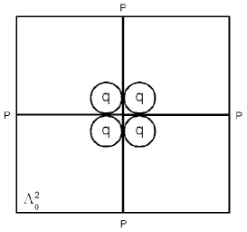
Figure 3. The period cell of $V_{\omega^{*}}$ in $d=2$.

On $\Lambda_{0}^{2}$ the potential $V_{\omega^{*}}$ is symmetric with respect to all hyperplanes $x_{i}=1/2$, $i=1,\ldots,d$. Thus $E_{0}^{per}$ coincides with the smallest eigenvalue of the Neumann problem on $\Lambda_{0}^{2}$. Again by symmetry of the potential, the latter coincides with the smallest eigenvalue of the Neumann problem on $\Lambda_{1}$. As $\omega_{0}^{*}=a^{*}$, this eigenvalue is $E_{0}(a^{*})$. Together with (7) we have shown that

$$E_{0}\leq\min\sigma(H_{\omega^{*}})=E_{0}(a^{*}).$$

Combined with the previous observation that $E_{0}(a^{*})\leq E_{0}$ this shows $E_{0}=\min\sigma(H_{\omega^{*}})$. ∎

4. Uniqueness of the Periodic Minimizer

After resolving the preliminary problem of characterizing the spectral minimum of the RDM, we could now turn to the other essential ingredients into a localization proof, a Lifshitz tail bound on the IDS and a Wegner estimate. However, a first look at this quickly demonstrates that we also need to address the question of uniqueness in Theorem 2.1. Other than translates of $\omega^{*}$, are there more periodic configurations which have the same spectral minimum?

To motivate this, let us include a first discussion of Lifshitz tails. For this one considers restrictions $H_{\omega,L}$ of $H_{\omega}$ to $L^{2}(\Lambda_{L})$, where $\Lambda_{L}$ is a cube of side-length $L$ centered at the origin. As boundary condition one can generally choose what is most convenient in a given model, for us this will be Neumann conditions. By a Lifshitz tail bound we mean a result which says that the probability of $H_{\omega,L}$ to have an eigenvalue close to $E_{0}$, the minimum of the infinite volume spectrum, is exponentially small in $L$. The meaning of “close” will be made more precise later.

If $\omega$ coincides with $\omega^{*}$ on $\Lambda_{L}$ or is very close to it, this will give a low lying eigenvalue of $H_{\omega,L}$. Our chances of getting a useful Lifshitz tail bound would worsen if there are many other periodic configurations with the same spectral minimum as $\omega^{*}$, as this would increase the probability that random configurations are close to one of the minimizing configurations on $\Lambda_{L}$ and thus have low lying eigenvalues.

From this it is immediately clear that for all further considerations we will have to assume that alternative (i) of Theorem 3.1 holds, as under alternative (ii) it follows that $H_{\omega,L}$ has spectral minimum $E_{0}$ for every configuration $\omega$. The following result is taken from [5].

Theorem 4.1.

Assume (A1), (A2), alternative (i) of Theorem 3.1, $d\geq 2$ and $r<1/4$. Then $\omega^{*}$ as given by (8) is, up to translations, the unique periodic configuration with $\min\sigma(H_{\omega^{*}})=E_{0}$.

Two additional assumptions were made here which deserve comment: For the “radius” $r$ of the single-site potential $q$ we require $r<1/4$ rather then just $r<1/2$ assumed earlier. This is a technical assumption, which we need to apply an analyticity argument in the proof, see below. Our guess is that this assumption is not necessary for Theorem 4.1 to hold.

However, Theorem 4.1 indeed only holds in the multi-dimensional case $d\geq 2$ In the case $d=1$ there are many periodic minimizers, as also proven in [5]:

Theorem 4.2.

Assume (A1), (A2), alternative (i) of Theorem 3.1 and $d=1$. Then an $L$-periodic configuration $\omega=(\omega_{n})_{n\in{\mathord{\mathbb{Z}}}}$, $\omega_{n+L}=\omega_{n}$ for all $n\in{\mathord{\mathbb{Z}}}$, satisfies $\min\sigma(H_{\omega})=E_{0}$ if and only if

(i) all $\omega_{n}$ are maximally displaced, i.e. $\omega_{n}=\pm d_{min}$ for all $n$,

(ii) $L$ is even, and

(iii) in each period $L$ equally many $\omega_{n}$ are displaced to the left and to the right.

It is easy to see that a periodic configuration $\omega$ with these properties is a minimizer. Let $\varphi_{0}$ be the positive ground state of $-d^{2}/dx^{2}+q(x-d_{max})$ on $(-1/2,1/2)$ with Neumann boundary conditions. It can be shown that alternative (i) implies that

$$h:=\varphi_{0}(-1/2)\not=\varphi_{0}(1/2)=:k.$$

For a configuration satisfying (i), (ii) and (iii) of Theorem 4.2 the Neumann ground state over the period $L$ is found by pasting together scaled copies of $\varphi_{0}$, compare Figure 4 for an example with $L=4$. The number of steps up is equal to the number of steps down, which allows for periodic extension, showing that $\min\sigma(H_{\omega})=E_{0}$.

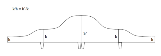
Figure 4. A 4-periodic minimizer in $d=1$.

Lemma 4.4 below, which holds in arbitrary dimension, establishes the necessity of (i). The above construction of the Neumann ground state for the period $L$ now shows that (ii) and (iii) must hold for the Neumann ground state to coincide with the periodic ground state. For a more detailed proof of Theorem 4.2 see [5].

Theorem 4.2 has surprising implications for the integrated density of states $N(E)$ of the one-dimensional RDM. The most extreme situation occurs if $\mu$ is the Bernoulli measure with equal weights at the endpoints of $[-d_{max},d_{max}]$, i.e.

$$\mu=\frac{1}{2}\delta_{d_{max}}+\frac{1}{2}\delta_{-d_{max}}.$$ (12)

Theorem 4.3.

Let $H_{\omega}$ be the one-dimensional RDM with distribution $\mu$ given by (12). Then there exists $C>0$ such that

$$N(E)\geq\frac{C}{(\log(E-E_{0}))^{2}}$$ (13)

for $E$ sufficiently close to $E_{0}$.

While similar phenomena have been found for Schrödinger operators with almost-periodic potentials, this is the first known example of a random Schrödinger operator with non-Hölder-continuous IDS. The density $n(E)=N^{\prime}(E)$ of eigenvalues near the bottom of the spectrum is even higher than for the one-dimensional Laplacian where the IDS has a square-root type singularity $N(E)=CE^{1/2}$ at $E_{0}=0$. Thus the randomness has the effect of pulling more eigenvalues towards the bottom of the spectrum, rather than pushing them away from the bottom as in the more common fluctuation boundary regime described by Lifshitz tails. The reason behind (13) is Theorem 4.2 combined with the law of large numbers. For the symmetric Bernoulli distribution (12) it has very high probability that in a large even period $L$ almost equally many $\omega_{n}$ take values $d_{max}$ and $-d_{max}$, leading to a ground state energy very close to $E_{0}$. For a detailed proof of Theorem 4.3 see [5].

We now turn back to the original goal of this section, the proof of Theorem 4.1 on the uniqueness of the periodic minimizer in $d\geq 2$. For this we consider a configuration $\omega\in{\mathcal{C}}_{per}$ (as defined in (6)) and let $\Lambda$ be the corresponding rectangular period cell. We let $H_{\omega,\Lambda}^{P}$ and $H_{\omega,\Lambda}^{N}$ be the restriction of $H_{\omega}$ to $L^{2}(\Lambda)$ with periodic and Neumann boundary conditions, respectively, and $E_{0}(H_{\omega,\Lambda}^{P})$ and $E_{0}(H_{\omega,\Lambda}^{N})$ their lowest eigenvalues. In follows from general facts that

$$\min\sigma(H_{\omega})=E_{0}(H_{\omega,\Lambda}^{P})\geq E_{0}(H_{\omega,\Lambda}^{N}).$$ (14)

We assume that $\min\sigma(H_{\omega})=E_{0}$ and have to show that, up to a translation, $\omega$ coincides with $\omega^{*}$. This is done in two steps.

The first step establishes that all $\omega_{n}$ sit in corners and that the ground state of $H_{\omega,\Lambda}^{N}$ satisfies Neumann conditions not only on $\Lambda$, but on every unit cell contained in $\Lambda$:

Lemma 4.4.

Let $\omega$ be a periodic configuration with $\min\sigma(H_{\omega})=E_{0}$. Then $\omega_{n}\in{\mathcal{C}}$ for all $n\in{\mathord{\mathbb{Z}}}^{d}$. Moreover, in this case $E_{0}(H_{\omega,\Lambda}^{P})=E_{0}(H_{\omega,\Lambda}^{N})$ and the ground state eigenfunction $\psi_{\omega}$ of $H_{\omega,\Lambda}^{N}$ satisfies Neumann boundary conditions on the boundary of each unit cube $\Lambda_{n}$ centered at $n\in\Lambda\cap{\mathord{\mathbb{Z}}}^{d}$.

The core of the proof of Lemma 4.4 is the following calculation, based on Neumann bracketing and the characterization of ground state energies as minimizers of the quadratic form:

$$E_{0}(H_{\omega,\Lambda}^{N}) = \frac{\int_{\Lambda}|\nabla\psi_{\omega}|^{2}+\int_{\Lambda}\sum_{n\in\Lambda\cap{\mathord{\mathbb{Z}}}^{d}}q(x-n-\omega_{n})|\psi_{\omega}|^{2}}{\int_{\Lambda}|\psi_{\omega}|^{2}}$$ (15)

$$= \sum_{n\in\Lambda\cap{\mathord{\mathbb{Z}}}^{d}}\frac{\int_{\Lambda_{n}}|\nabla\psi_{\omega}|^{2}+\int_{\Lambda_{n}}q(x-n-\omega_{n})|\psi_{\omega}|^{2}}{\int_{\Lambda_{n}}|\psi_{\omega}|^{2}}\cdot\frac{\int_{\Lambda_{n}}|\psi_{\omega}|^{2}}{\int_{\Lambda}|\psi_{\omega}|^{2}}$$

$$\geq \sum_{n\in\Lambda\cap{\mathord{\mathbb{Z}}}^{d}}E_{0}(\omega_{n})\frac{\int_{\Lambda_{n}}|\psi_{\omega}|^{2}}{\int_{\Lambda}|\psi_{\omega}|^{2}}\geq\sum_{n\in\Lambda\cap{\mathord{\mathbb{Z}}}^{d}}E_{0}\frac{\int_{\Lambda_{n}}|\psi_{\omega}|^{2}}{\int_{\Lambda}|\psi_{\omega}|^{2}}=E_{0},$$

By (14) and the assumption we conclude that $E_{0}(H_{\omega,\Lambda}^{P})=E_{0}(H_{\omega,\Lambda}^{N})$ and that all inequalities in (15) are equalities. We also see that $\omega_{n}\in{\mathcal{C}}$ for all $n\in{\mathord{\mathbb{Z}}}^{d}$, because otherwise, given alternative (i), the last inequality in (15) would be strict. Finally we see from equality in the second to last inequality in (15) that $\psi_{\omega}|_{\Lambda_{n}}$ is the ground state for the Neumann problem on $\Lambda_{n}$, and thus satisfies Neumann conditions on $\Lambda_{n}$.

The second step of the proof of Theorem 4.1 is to show symmetric matching of the bubbles, i.e. that in each pair of neighboring unit cells within $\Lambda$ the single-site potentials are placed symmetrically with respect to the common boundary of the cells. For this we use the following general fact from [5], to where we refer for the proof:

Lemma 4.5.

Consider a connected open region $D$ in ${\mathord{\mathbb{R}}}^{d}$, $d\geq 2$ and a hyperplane $P$ that divides this region into two nonempty subregions. Denote by $\sigma$ the reflection about $P$ and assume that $D\cap\sigma(D)$ is connected. Let $E\in{\mathord{\mathbb{R}}}$ and, in $D$, let $u$ be a solution of the equation

$$-\Delta u=Eu$$ (16)

which satisfies the condition $\frac{\partial u}{\partial n}=0$ on $P\cap D$. Then $u$ can be extended to a symmetric function $w$ on $D\cup\sigma(D)$ which satisfies the equation $-\Delta u=Eu$ in this region.

To finish the proof of Theorem 4.1 let us assume that $\omega$ is a periodic minimizing configuration in which, by Lemma 4.4, all bubbles sit in corners, but that there is at least one non-matching neighboring pair of bubbles. Let us focus on $d=2$ and the situation in Figure 5 (the general argument in [5] uses the same idea).

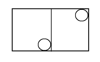
Figure 5. A non-matching pair.

Circumscribe squares around the supports of the two bubbles and remove these two squares from the union $R$ of the two cells. Choose the resulting region as $D$ in Lemma 4.5, and $\sigma$ as reflection at the center line. Here (and only here) we need the strengthened assumption $r<1/4$ in Theorem 4.1 to make sure that $D\cap\sigma(D)$ is connected.

Let $u$ be the restriction of the ground state of $H_{\omega,\Lambda}^{N}$ to $D$. Then $-\Delta u=E_{0}u$ on $D$ and, by Lemma 4.4, $u$ satisfies Neumann conditions on the centerline $P\cap D$. By Lemma 4.5 $u$ can be extended to a symmetric function $w$ on $D\cup\sigma(D)$ satisfying $-\Delta w=E_{0}w$. But $D\cup\sigma(D)=R$ and thus $w$ is the ground state of the Neumann Laplacian on $R$, implying $E_{0}=0$ and that $w$ is constant, a contradiction to alternative (i). This completes the proof of Theorem 4.1.

To end this section let us remark that the fundamental difference in the one-dimensional and multi-dimensional case lies in the possibility to smoothly match Neumann ground states on different unit cells. In $d=1$ this can always be done by re-scaling as explained by Figure 5. In higher dimension the boundary of cells has much more structure (is not just a point), which ultimately results in matching of ground states only being possible in the trivial reflection-symmetric case.

5. Special Lifshitz tails

After clarifying uniqueness questions in the previous section we finally have enough background information to enter into a discussion of Lifshitz tail properties of the IDS for the random displacement model. In order to use our earlier results we will have to assume from here on that alternative (i) of Theorem 3.1 holds and that $d\geq 2$. We strengthen (A2) to require $r<1/4$ and will in this section also assume that $q$ is continuous to make use of results in [35].

Let $H_{\omega,L}^{N}$ be the restriction of $H_{\omega}$ to $\Lambda_{L}=(-L-1/2,L+1/2)^{d}$ with Neumann boundary conditions. The crucial fact required in localization proofs and also in the proof of Lifshitz tail asymptotics of the IDS is that the probability of $H_{\omega,L}^{N}$ having an eigenvalue close to $E_{0}$ is very small. The first proof of this was given in [35], where it follows as a special case of a more general result. The methods derived in [35] require to assume in (A2) that supp$\,\mu$ is finite. The methods developed later in [30], which are described in Section 7 below, have allowed to remove this additional assumption on $\mu$. However, Theorem 5.1 is crucial as it will serve as the anchor for a bootstrap argument in Section 7. For this it will be sufficient to start with the case supp$\,\mu={\mathcal{C}}$, i.e. a displacement model where all bubbles sit in corners.

Theorem 5.1.

Let the assumptions listed at the beginning of this section be satisfied and also assume that supp$\,\mu={\mathcal{C}}$. Then there exist $C>0$ and $\mu>1$ such that for all $L\in{\mathord{\mathbb{N}}}$,

$${\mathord{\mathbb{P}}}\left(\min\sigma(H_{\omega,L}^{N})<E_{0}+\frac{C}{L^{2}}\right)<(2L+1)^{d-1}\mu^{-2L}.$$ (17)

In the remainder of this section we will discuss the argument from [35] which proves Theorem 5.1, taking some advantage in presentation from only looking at the specific situation which is of interest to us here. However, we will refer to [35] for many of the core analytical parts of the proof.

The argument starts with decomposing the cubes $\Lambda_{L}$ into quasi-one-dimensional tubes (see Figure 6) and restricting $H_{\omega,L}^{N}$ to these tubes under insertion of additional Neumann boundary conditions.

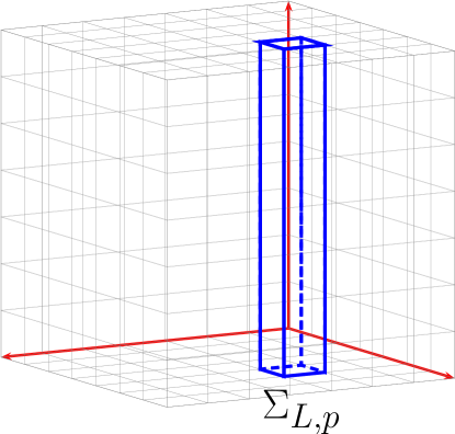
Figure 6. A quasi-one-dimensional tube

Thus let

$$\hskip-170.71652ptA_{L}:=\{p\in{\mathord{\mathbb{Z}}}^{d-1}:-L\leq p_{j}\leq L\;\mbox{for}\;j=1,\ldots,d-1\}$$

and, for each $p\in A_{L}$,

$$\hskip-170.71652pt\Sigma_{L,p}:=\bigcup_{k=-L}^{L}\Lambda_{1}((p,k)),$$

with $\Lambda_{1}((p,k))$ denoting unit cubes centered at $(p,k)\in{\mathord{\mathbb{Z}}}^{d}$. By $H_{\omega,L,p}^{N}$ we denote the restriction of $H_{\omega}$ to $L^{2}(\Sigma_{L,p})$ with Neumann boundary conditions. By Neumann bracketing we have

$$H_{\omega,L}^{N}\geq\bigoplus_{p\in A_{L}}H_{\omega,L,p}^{N}$$

and therefore

$$\min\sigma(H_{\omega,L}^{N})\geq\min_{p\in A_{L}}\min\sigma(H_{\omega,L,p}^{N}).$$ (18)

For a given $\omega$ such that $\omega_{n}\in{\mathcal{C}}$ for all $n$ we will say that two neighboring unit cubes are matching if the single site potentials in the two cubes are mirror images under reflection at the common boundary of the cubes. For each $p\in A_{L}$ consider the event

$$X_{L,p}:=\{\omega:\Sigma_{L,p}\;\mbox{contains at least one neighboring pair of non-matching cubes}\}$$

and let $X_{L}:=\cap_{p\in A_{L}}X_{L,p}$.

By independence we have

$${\mathord{\mathbb{P}}}(\omega\notin X_{L,p})\leq\mu^{-2L},$$

where $\mu:=1/\max_{a\in{\mathcal{C}}}\mu(a)$ (after $\omega_{p,-L}$ is chosen, the other $2L$ values of $\omega_{p,k}$ are determined by matching). This implies that

$${\mathord{\mathbb{P}}}(X_{L})\geq 1-(2L+1)^{d-1}\mu^{-2L}.$$ (19)

If $\omega\in X_{L}$, then each tube $\Sigma_{L,p}$ contains at least one non-matching pair of neighboring cubes. Thus by Proposition 5.2 below $\min\sigma(H_{\omega,L,p}^{N})\geq E_{0}+C/L^{2}$ for a $C>0$ independent of $p$ and $L$. Thus Theorem 5.1 follows from (18) and (19).

In the proposition which was used here we can without loss consider $p=0$:

Proposition 5.2.

There is a constant $C>0$, independent of $L$, such that for every $\omega$ with $\omega_{n}\in{\mathcal{C}}$ for all $n$ and at least one non-matching pair of cubes in $\Sigma_{L,0}$ it holds that

$$\min\sigma(H_{\omega,L,0})\geq E_{0}+\frac{C}{L^{2}}.$$ (20)

This, at least essentially, is a result proven in [35]. We will not reproduce the details of the proof, which involve a surprisingly rich combination of analysis tools such as a Poincaré-type inequality, the so-called ground state transform and properties of a Dirichlet-to-Neumann operator, as well as some combinatorics. But we will outline the main idea:

The proof of Proposition 5.2 starts by first arguing that is suffices to assume that

1. the first two cubes $\Lambda_{1}((0,-L))$ and $\Lambda_{1}((0,-L+1))$ are non-matched, while

2. all other neighboring pairs are matched.

Seeing this is not entirely trivial and requires a trick as well as some combinatorics. The trick consists in extending the operator $H_{\omega,L,0}^{N}$ by reflection to a twice longer tube and to consider the resulting operator as an operator on the torus $[-1/2,1/2]^{d-1}\times({\mathord{\mathbb{R}}}/2(2L+1){\mathord{\mathbb{Z}}})$ with periodic boundary conditions. Due to symmetry this operator has the same spectral minimum as $H_{\omega,L,0}^{N}$. Now one argues that the torus can be decomposed into subsegments each of which has a non-matching pair of cubes at one end and otherwise only matching pairs of cubes. Introducing additional Neumann conditions on the subsegments lowers the spectrum and it now suffices to prove the claim for each subsegment (which has length bounded by $2(2L+1)$). Justifying that this decomposition is possible “is an easy combinatorics, though somewhat lengthy to write down using symbols”, where we use the words of [35] and omit the details.

Under the additional assumptions (1), (2), Proposition 5.2 is essentially a special case of Theorem 2.1 in [35]. While our situation does not satisfy the exact symmetry assumptions of Theorem 2.1 in [35], the construction of our potential via matching cubes allows to mimic the proof in [35] almost line by line. (We mention, however, that Section 4 of [35] provides a slightly different argument which allows to directly use their Theorem 2.1 to prove Theorem 5.1 above.)

Here the results of Section 4 enter as follows: As the first pair of cubes $\Lambda_{1}((0,-L))$ and $\Lambda_{1}((0,-L+1))$ does not match, the lowest eigenvalue of the Neumann problem on the union $\Lambda_{2}$ of these two cubes is strictly larger than $E_{0}$. This follows from the arguments in the proof of Theorem 4.1, more specifically the argument at the end of Section 4 which ruled out that in this situation the lowest eigenvalue can be equal to $E_{0}$. It is this operator which plays the role of the operator $P_{0}^{N}$ in [35]. By the results of Section 4 it is clear that inserting an additional Neumann condition along the surface separating $\Lambda_{2}$ and $\Sigma_{L,0}\setminus\Lambda_{2}$ strictly lowers the ground state energy of $H_{\omega,L,0}^{N}$ to $E_{0}$. The meaning of Theorem 2.1 of [35] is that it provides the quantitative lower bound $CL^{-2}$ on how much the energy is lowered depending on the length of the attached tube.

The value of the constant $C>0$ in (20) which is provided by the argument in [35] will depend on the choice of $\omega_{0,-L}$ and $\omega_{0,-L+1}$, after which the remaining values of $\omega_{n}$ are determined by matching. However, as only the finitely many values in the corners ${\mathcal{C}}$ are allowed, one can ultimately choose the smallest of finitely many values of $C$.

As indicated earlier, Theorem 5.1 is the result which will be used later, rather than its consequences for the IDS $N(E)$ of $H_{\omega}$. However, we mention that the following Lifshitz tail bound can be derived from Theorem 5.1 with standard arguments, see [35]:

$$\limsup_{E\downarrow E_{0}}\frac{\log|\log N(E)|}{\log(E-E_{0})}\leq-\frac{1}{2}.$$ (21)

The Lifshitz exponent $-1/2$ obtained here is likely not optimal. One would expect that the correct exponent is $-d/2$, as known for the Anderson model or Poisson model. The reason for the discrepancy lies in the essentially one-dimensional argument which enters the proof through the decomposition of cubes into quasi-one-dimensional tubes.

We stress the fundamentally different low energy behavior of the IDS of the RDM in the one-dimensional and multi-dimensional settings. If supp$\,\mu={\mathcal{C}}$ with equal probability for all corners, then (21) shows that the IDS has a very thin tail for $d\geq 2$, while by Theorem 4.3 it has a very fat tail (and thus the spectrum does not have a fluctuation boundary) for $d=1$. From this point of view it is a fortunate coincidence that our main goal here is to prove localization in $d\geq 2$ and that, as discussed in the Introduction, localization for the one-dimensional case was already settled by very different methods.

6. The Missing Link

It is tempting to believe at this point of our work that we are halfway done with verifying the necessary ingredients for a multiscale analysis proof of localization for the RDM. Under suitable assumptions we have shown the Lifshitz-tail bound (17), so it remains to establish a Wegner estimate. Unfortunately, the assumption that supp$\,\mu$ be finite in Theorem 5.1 makes us face a dilemma: Most known proofs of Wegner-type estimates, with the exception of some results in $d=1$ [9, 13], require some smoothness or at least continuity of the distribution of the random parameters, due to the use of averaging techniques involving only finitely many random parameters. For the multi-dimensional continuum Anderson model with Bernoulli distributed random coupling constants a localization proof near the bottom of the spectrum was enabled only recently by the powerful extension of multiscale analysis presented in [6], see also [2] for an extension to the case of arbitrary single site distributions and [21] for a detailed elaboration of the intricate ideas behind [6]. One of the main features of this approach is that the Wegner estimate is not established as an a-priori-ingredient, but its proof is part of the multiscale iteration procedure leading to localization. We mention that due to the use of unique continuation arguments this approach does not work on the lattice, leaving the proof of localization for the multi-dimensional discrete Bernoulli-Anderson model an open problem.

Thus, if we want to complete a localization proof for the RDM based on “traditional” multiscale analysis, the proof of a Wegner estimate will likely require a sufficient amount of regularity of the distribution $\mu$ of the displacement parameters $\omega_{n}$. But this means that we also need to extend the Lifshitz-tail bound to more general distributions $\mu$. The proof discussed in Section 5 above does not extend to this case, as it would require to take an infimum over infinitely many positive constants $C$ with insufficient quantitative information available to guarantee that the resulting constant is strictly positive.

It turned out that the missing link which allowed to overcome both remaining problems, the extension of the Lifshitz-tail bound to a larger class of distributions and the proof of a Wegner estimate for this class, is provided by an inconspicuous but crucial improvement on how bubbles tend to the corners, meaning Theorem 3.1. There it was shown that the function $E_{0}(a)$, as long as it does not vanish identically, is strictly decreasing in each of its variables away from the origin. The crucial improvement is that this decrease arises in the form of non-vanishing derivative.

This is the first instance where we will have to require some smoothness of $q$, as differentiability of $E_{0}(\cdot)$ requires differentiability of $q$ via perturbation theory, see Section 2.1 of [30]. For convenience, we will assume that $q$ is $C^{\infty}$, even if much less is needed below and in the rest of this paper.

As this is the last time we add assumptions on $q$, let us restate the full set:

(A1)’ The single-site potential $q:{\mathord{\mathbb{R}}}^{d}\to{\mathord{\mathbb{R}}}$ is infinitely differentiable, reflection-symmetric in each variable and such supp$\,q\subset[-r,r]^{d}$ for some $r<1/4$. Also assume that $E_{0}(a)=\min\sigma(H_{\Lambda_{1}}^{N}(a))$ does not vanish identically in $a\in\overline{G}$.

We now get

Theorem 6.1.

Assume (A1)’. Then for all $a=(a_{1},\ldots,a_{d})\in\overline{G}$ and all $i=1,\ldots,d$ we have

$$\partial_{i}E_{0}(a)\left\{\begin{array}[]{ll}<0,&\mbox{if $a_{i}>0$},\\ =0,&\mbox{if $a_{i}=0$},\\ >0,&\mbox{if $a_{i}<0$}.\end{array}\right.$$

The proof of Theorem 6.1 is far from obvious (at least to us) and is best discussed in the larger context of considering similar questions for more general domains $G$. In order to not interrupt the presentation of our main story, i.e. the proof of localization for the random displacement model, we postpone this discussion to Section 10 below. But let us point out that the step from Theorem 3.1 to Theorem 6.1 turned out to be far from straightforward. The “smooth methods” behind the proof of Theorem 6.1 are very different from the symmetry-based operator theoretic methods used to prove Theorem 3.1 in [4] and, in particular, explicitly use second order perturbation theory.

7. General Lifshitz tails

The first of two important applications of Theorem 6.1 is that it allows us to extend the Lifshitz tail bound found in Theorem 5.1 to general distributions $\mu$, not requiring finiteness of the support.

Theorem 7.1.

Assume that $q$ and $\mu$ satisfy (A1)’ and (A2). Then there exist $C_{1}>0$ and $\mu>1$ such that

$${\mathord{\mathbb{P}}}\left(\min\sigma(H_{\omega,L}^{N})<E_{0}+\frac{C_{1}}{L^{2}}\right)\leq(2L+1)^{d-1}\mu^{-2L}$$ (22)

for all $L\in{\mathord{\mathbb{N}}}$.

We will prove this result by comparing the quadratic form of $H_{\omega,L}^{N}$ with the quadratic form of a modified displacement model where all bubbles have been moved to the closest corner within their cell. Thus, for $a\in\overline{G}$, let $c(a)\in{\mathcal{C}}$ be the corner closest to $a$ (if several corners are equally close, any of them can be chosen). For a displacement configuration $\omega=(\omega_{n})_{n\in{\mathord{\mathbb{Z}}}^{d}}\in\overline{G}^{{\mathord{\mathbb{Z}}}^{d}}$, define $c(\omega)\in\overline{G}^{{\mathord{\mathbb{Z}}}^{d}}$ by $(c(\omega))_{n}=c(\omega_{n})$.

From Theorem 3.1 we know that the single-site operator $H_{\Lambda_{1}}^{N}(c(a))$ has lower ground state energy than $H_{\Lambda_{1}}^{N}(a)$. Theorem 6.1 allows us to quantify this, saying that the distance of the two ground state energies is proportional to $|a-c(a)|$. In particular, there exists $C_{2}\in(0,\infty)$ such that

$$E_{0}(a)-E_{0}\geq\frac{1}{C_{2}}D(a),$$ (23)

where $D(a)=\min_{c\in{\mathcal{C}}}|a-c|$. This is one of the two central ingredients in the proof of the following result. The other one will be Neumann bracketing.

Proposition 7.2.

There exists a constant $C_{3}\in(0,\infty)$ such that, in the sense of quadratic forms,

$$H_{\omega,L}^{N}-E_{0}\geq\frac{1}{C_{3}}(H_{c(\omega),L}^{N}-E_{0}).$$ (24)

for all $\omega\in\overline{G}^{{\mathord{\mathbb{Z}}}^{d}}$ and all $L\geq 0$.

In particular, (24) implies

$$\min\sigma(H_{\omega,L}^{N})-E_{0}\geq\frac{1}{C_{3}}(\min\sigma(H_{c(\omega),L}^{N}-E_{0}).$$ (25)

The RDM $H_{c(\omega)}$ has i.i.d. distributed displacements supported on $\mathcal{C}$ and thus satisfies the assumptions of Theorem 5.1. Therefore, with $C$ and $\mu$ from Theorem 5.1,

$${\mathord{\mathbb{P}}}\left(\min\sigma(H_{\omega,L}^{N})-E_{0}<\frac{C}{C_{3}L^{2}}\right)\leq{\mathord{\mathbb{P}}}\left(\min\sigma(H_{c(\omega),L}^{N})-E_{0}<\frac{C}{L^{2}}\right)\leq(2L+1)^{d-1}\mu^{-2L},$$

proving Theorem 7.1.

Thus it remains to prove Proposition 7.2. The strategy for this is to first prove a corresponding result for the single-site operators $H_{\Lambda_{1}}^{N}(a)$ and then extend this by Neumann bracketing to the operators $H_{\omega,L}^{N}$. For the single-site operators one separately considers the cases where $a$ is close to a corner or not close to a corner.

Lemma 7.3.

There exist $C>0$ and $\delta>0$ such that, if $D(a)\leq\delta$, then

$$H_{\Lambda_{1}}^{N}(a)-E_{0}\geq\frac{1}{C}(H_{\Lambda_{1}}^{N}(c)-E_{0}+|a-c|).$$ (26)

Lemma 7.4.

Fix $\delta\in(0,1)$. There exists $C_{\delta}\in(0,\infty)$ such that, for $D(a)\geq\delta$ and all $c\in{\mathcal{C}}$,

$$H_{\Lambda_{1}}^{N}(a)-E_{0}\geq\frac{1}{C_{\delta}}(H_{\Lambda_{1}}^{N}(c)-E_{0}+|a-c|).$$ (27)

Before discussing the proofs of the two Lemmas, let us show how we use them to prove Proposition 7.2. Note that, applying Lemma 7.4 with $\delta$ as provided in Lemma 7.3, both Lemmas combined prove the $L=0$ case. To extend this to general boxes we employ an argument previously used in the proof of Theorem 2.1 in [34]. It is crucial here that we work with Neumann boundary conditions.

For $\psi\in H^{1}(\Lambda_{2L+1})$, the form domain of $H_{\omega,L}^{N}$, one has that the restriction of $\psi$ to $\Lambda_{1}(n)$ is in $H^{1}(\Lambda_{1}(n))$ for each $n\in\Lambda_{2L+1}^{\prime}:=\Lambda_{2L+1}\cap{\mathord{\mathbb{Z}}}^{d}$. Moreover,

$$\langle(H_{\omega,L}^{N}-E_{0})\psi,\psi\rangle=\sum_{n\in\Lambda_{2L+1}^{\prime}}\langle(H_{\Lambda_{1}(n)}^{N}(\omega_{n})-E_{0})\psi,\psi\rangle,$$

where we work with the usual slightly abusive notation for quadratic forms.

The same argument may be applied to $H_{c(\omega)}$,

$$\langle(H_{c(\omega),L}^{N}-E_{0})\psi,\psi\rangle=\sum_{n\in\Lambda_{2L+1}^{\prime}}\langle(H_{\Lambda_{1}(n)}^{N}(c(\omega_{n}))-E_{0})\psi,\psi\rangle.$$

Now Proposition 7.2 follows by applying Lemmas 7.3 and 7.4 for each $n$, summing, and omitting the positive term $\sum_{n}\langle|\omega_{n}-c(\omega_{n})|\psi,\psi\rangle_{\Lambda_{1}(n)}$.

Before we can end this section, we still owe a discussion of the proofs of Lemmas 7.3 and 7.4. To see the latter, note that $D(a)\geq\delta$ implies $H_{\Lambda_{1}}^{N}(a)-E_{0}\geq\delta/C_{2}$ by (23). Using the rough bound $|q(x-a)-q(x-c)|\leq 2\|q\|_{\infty}$ and setting $C:=1+2C_{2}\|q\|_{\infty}/\delta$ we get

$$(C+1)(H_{\Lambda_{1}}^{N}(a)-E_{0})-(H_{\Lambda_{1}}^{N}(c)-E_{0})\geq\frac{C\delta}{C_{2}}-2\|q\|_{\infty}=\frac{\delta}{C_{2}},$$

and thus

$$H_{\Lambda_{1}}^{N}(a)-E_{0}\geq\frac{1}{C+1}\left(H_{\Lambda_{1}}^{N}(a)-E_{0}+\frac{\delta}{C_{2}}\right).$$

As $\delta=\frac{\delta}{|a-c|}|a-c|\geq\frac{\delta}{2d_{max}\sqrt{d}}|a-c|$, (27) follows with $1/C_{\delta}$ chosen as the smaller of $1/(C+1)$ and $\delta/(2(C+1)C_{2}d_{max}\sqrt{d})$.

The previous argument doesn’t use the full strength of (23), but only that $E_{0}(\cdot)$ is continuous and strictly minimized in the corners. The proof of Lemma 7.3 is more subtle and depends on the linear growth of $E_{0}(\cdot)$ away from the corners. To $a\in\overline{G}$ pick $c\in{\mathcal{C}}$ such that $D(a)=|a-c|$. By smoothness of $q$ we have the Taylor approximation $q(\cdot-a)-q(\cdot-c)=(c-a)\cdot\nabla q(\cdot-c)+o(|a-c|)$ and thus

$$H_{\Lambda_{1}}^{N}(c)-E_{0}=H_{\Lambda_{1}}^{N}(c)-E_{0}+(c-a)\cdot\nabla q(\cdot-c)+o(|a-c|).$$ (28)

Bounding the left hand side by (23) we get, in the sense of quadratic forms,

$$H_{\Lambda_{1}}^{N}(c)-E_{0}+(c-a)\cdot\nabla q(\cdot-c)\geq\frac{1}{C_{2}}|a-c|+o(|a-c|).$$

Hence, for $\rho\in(0,1)$ sufficiently small and $\sigma\in{\mathcal{S}}^{d-1}$ with $a=c+\rho\sigma\in\overline{G}$,

$$H_{\Lambda_{1}}^{N}(c)-E_{0}-\rho\sigma\cdot\nabla q(\cdot-c)\geq\frac{\rho}{2C_{2}}.$$

We apply Lemma 7.5 below with $A=H_{\Lambda_{1}}^{N}(c)-E_{0}$ and $B=-\rho\sigma\cdot\nabla q(\cdot-c)$ to conclude that for $C_{\rho}=\max(2,2C_{2}/\rho)$ $t\in[0,1/2]$ and $\sigma\in{\mathcal{S}}^{d-1}$ with $c+\rho\sigma\in\overline{G}$,

$$H_{\Lambda_{1}}^{N}(c)-E_{0}-t\rho\sigma\cdot\nabla q(\cdot-c)\geq\frac{1}{C_{\rho}}(H_{\Lambda_{1}}^{N}(c)-E_{0}+t).$$

From this and (28) we find for $|a-c|\leq\rho/2$ and $t=|a-c|/\rho$,

$$H_{\Lambda_{1}}^{N}(a)-E_{0}\geq\frac{1}{C_{\rho}}(H_{\Lambda_{1}}^{N}(c)-E_{0}+|a-c|/\rho)+o(|a-c|).$$

This implies (26) if $\delta>0$ is chosen sufficiently small, completing the proof of Lemma 7.3.

We have used the following simple fact, which was previously used in a similar context in [34].

Lemma 7.5.

Let $A$ be self-adjoint and $B$ bounded and self-adjoint with $A\geq 0$ and $A+B\geq c_{0}>0$, then

$$A+tB\geq\min(\frac{1}{2},c_{0})\cdot(A+t)$$

for all $t\in[0,1/2]$.

This is elementary:

$$A+tB=(1-t)A+t(A+B)\geq\frac{1}{2}A+tc_{0}\geq\min(\frac{1}{2},c_{0})(A+t).$$

8. Wegner Estimate

To describe the ideas behind the proof of a Wegner estimate, we consider $H^{r}_{\omega}$, a suitable random Schrödinger operator on $L^{2}({\mathord{\mathbb{R}}}^{d})$. Let $L>0$ and $H^{r}_{\omega,L}$ be the restriction of $H^{r}_{\omega}$ to the cube $\Lambda_{L}$ with, say, Dirichlet boundary conditions. The boundary conditions are expected not to play a too important role.

A Wegner estimate (see [41]) is an estimate on

$$\mathbb{E}({\mathop{\rm tr\ }}\chi_{[E_{0}-\varepsilon,E_{0}+\varepsilon]}(H^{r}_{\omega,L}))=\mathbb{E}({\#\{\text{eigenvalues of }H^{r}_{\omega,L}\text{ in }[E_{0}-\varepsilon,E_{0}+\varepsilon]\}})$$ (29)

for $L$ large, $\varepsilon$ small and a fixed energy $E_{0}$. It can also take the form of an estimate on the probability $\mathbb{P}\{H^{r}_{\omega,L}\text{ has an eigenvalue in }[E_{0}-\varepsilon,E_{0}+\varepsilon]\}$ which, by Chebyshev’s inequality, is smaller than the previous quantity.

From their very form, it is clear that both quantities should increase with $\varepsilon$ and with $L$. The existence of an integrated density of states for $H_{\omega}^{r}$ suggests that the optimal upper bound should be proportional to $|\Lambda_{L}|\sim L^{d}$. The optimal upper bound in $\varepsilon$ is related to the regularity of the integrated density of states. The best bound one may expect is of the form $C\varepsilon L^{d}$.

Let us give the heuristic underlying such a bound in the simplest case, the case when $H^{r}_{\omega}$ is the continuous Anderson type model $H^{A}_{\lambda(\omega)}$ defined in (2), when $q$ has a fixed sign, say, positive, is continuous and bounded, its support contains $\Lambda_{1}$ and the coupling constants $(\lambda_{n})_{n\in{\mathord{\mathbb{Z}}}^{d}}$ are i.i.d. and bounded.

Let $(E_{j}(\omega,L))_{j}$ denote the eigenvalues of $H^{A}_{\lambda(\omega),L}$ ordered increasingly. To estimate the quantity $\mathbb{E}({\mathop{\rm tr\ }}\chi_{[E_{0}-\varepsilon,E_{0}+\varepsilon]}(H^{A}_{\lambda(\omega),L}))$, we can write

$$\mathbb{E}({\mathop{\rm tr\ }}\chi_{[E_{0}-\varepsilon,E_{0}+\varepsilon]}(H^{A}_{\omega,L})) =\mathbb{E}\left(\sum_{j}\chi_{[E_{0}-\varepsilon,E_{0}+\varepsilon]}(E_{j}(\omega,L))\right)$$

$$\leq\sum_{j\in N_{L}}\mathbb{P}\left\{E_{j}(\omega,L)\in[E_{0}-\varepsilon,E_{0}+\varepsilon]\right\}.$$

where, by standard bounds on Schrödinger operators, $\#N_{L}\lesssim L^{d}$.

In the case of the continuous Anderson model under the assumptions made above, for $\alpha>0$, the operator inequality $H^{A}_{\lambda(\omega)+\overline{\alpha}}-H^{A}_{\lambda(\omega)}\gtrsim\alpha$ tells us that

$$\forall j,\quad E_{j}(\lambda(\omega)+\overline{\alpha},L)-E_{j}(\lambda(\omega),L)\gtrsim\alpha,$$ (30)

where $\overline{\alpha}$ is the vector whose entries are all $\alpha$.

Based on this and under the assumption that the distribution of the $\lambda_{n}$ has a bounded density one can prove that

$$\forall j,\quad\mathbb{P}\left\{E_{j}(\omega,L)\in[E_{0}-\varepsilon,E_{0}+\varepsilon]\right\}\lesssim\varepsilon$$ (31)

and obtains the desired bound in $\varepsilon L^{d}$. The proof of (31), while essentially based on the ideas described above, requires additional technical work.

For the discrete $d$-dimensional Anderson model, the bound

$$\mathbb{E}({\mathop{\rm tr\ }}\chi_{[E_{0}-\varepsilon,E_{0}+\varepsilon]}(H^{r}_{\omega,L}))\leq C\varepsilon L^{d}$$ (32)

essentially goes back to Wegner’s original paper [41], with some technical details filled in later. A detailed proof, essentially following Wegner’s orginal argument, can be found, for example, in the recent survey [28]. Obtaining the bound (32) for the continuum Anderson model was harder, as one can not use the same rank one perturbation methods as in the discrete case to control the spectral shift due to single site terms. Initially, a bound of the form $C\varepsilon L^{2d}$ was obtained for the continuum Anderson model in [27] (for a proof with slightly different methods see also [38]). For $q$ of fixed sign, but without the assumption that the support of $q$ contains $\Lambda_{1}$ and at arbitrary energy, the linear in volume bound (32) was ultimately obtained in [11].

To describe how a Wegner estimate for the random displacement model considered here was found, let us describe a generalization of the idea outlined above which goes back to [31, 32, 33]. To estimate $\mathbb{P}\{E_{j}(\omega,L)\in[E_{0}-\varepsilon,E_{0}+\varepsilon]\}$, we study the mapping $\omega\mapsto E_{j}(\omega,L)$ that realizes a “projection” from the parameter (probability) space onto the real axis; and we want to measure the size (with respect to the probability measure on the parameter space) of the pre-image of some interval. The idea is then to find a vector field ${\mathcal{V}}$ in the parameters $\omega$ such that the eigenvalue $E_{j}(\omega,L)$ moves when $\omega$ moves along the flow of the vector field.

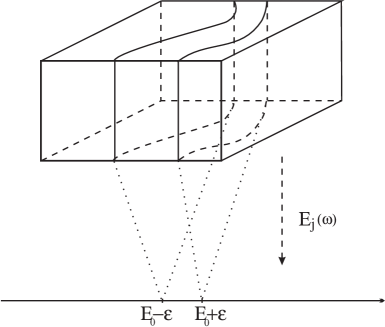
Figure 7. Foliation and projection of the probability space

The flow of ${\mathcal{V}}$ foliates the parameter space nicely and the volume we want to measure is just the volume contained in a layer between two leaves (see Figure 7). This volume will then be of size the width of this layer at least when the probability measure has a regular density. So if one is able to do this for all the eigenvalues, one gets an estimate of the form $\varepsilon L^{d}$.

To be able to do this for all eigenvalues at a time, one may choose ${\mathcal{V}}$ so that $H_{\omega}^{r}$ differentiated along ${\mathcal{V}}$ has nice properties (e.g. positivity). Let us take the simple example of the continuous Anderson Hamiltonian under the assumptions made above. If we take $\displaystyle{\mathcal{V}}=\text{div}_{\lambda(\omega)}=\sum_{n\in\Lambda_{L}}\frac{\partial}{\partial\lambda_{n}(\omega)}$, then ${\mathcal{V}}H_{\lambda(\omega)}^{L}\gtrsim\chi_{\Lambda_{L}}$. This ensures ${\mathcal{V}}E_{j}(\omega,L)\gtrsim 1$ which is exactly (30). This is what is needed for a Wegner estimate for the continuous Anderson Hamiltonian when the single site coupling constants admit a bounded density.

The right choice of vector field is model dependent; for the Anderson model, discrete or continuous, in many cases, one may use the divergence vector field as above (for example, see [41, 38]). Another useful vector field with respect to this problem is the generator of the dilations $\sum_{n}\lambda_{n}(\omega)\partial_{\lambda_{n}(\omega)}$. It can be used to get a Wegner estimate for the continuous Anderson model without sign assumptions on $V$ [32, 24] and, in certain cases, for the random displacement models [22]. Other types of randomness may require different types of vector fields, see e.g. [31, 15].

For the random displacement Hamiltonian $H_{\omega}$, we will use the same idea and introduce a new vector field. The choice of this vector field is motivated by Theorems 3.1 and 6.1, which indicate that at least low lying eigenvalues should decrease monotonically if the single site potentials are moved towards a corner of their cell.

For a function $f$ on $G$ we set

$$(\partial_{c}f)(a):=\frac{c(a)-a}{|c(a)-a|}\cdot\nabla f(a),$$

with $c(a)$ denoting the corner closest to $a$ as in Section 7. Thus, $\partial_{c}$ denotes the directional derivative in the direction of the closest corner, where points $a$ with multiple closest corners will not play a role in the arguments below (starting from (34) below we introduce a cut-off which restricts the values of $a$ relevant for the proof to small neighborhoods of the corners).

By Theorem 6.1 there exist $\delta_{0}>0$ and $r_{0}>0$ such that

$$\partial_{c}E_{0}(a)\leq-\delta_{0}\quad\mbox{for all $a\in A_{r_{0}}:=\{a\in G:|c(a)-a|\leq r_{0}\}$},$$ (33)

a neighborhood of $\mathcal{C}$.

Let $\eta\in C^{\infty}(\mathbb{R})$ such that $0\leq\eta\leq 1$, $\eta(r)=1$ for $r\leq r_{0}$ and $\eta(r)=0$ for $r\geq 2r_{0}$. Using this function as a cut-off, we localize the vector fields associated with $\partial_{c}$ onto a neighborhood of the corners, defining

$$(\partial^{\prime}_{c}f)(a):=\eta(|c(a)-a|)(\partial_{c}f)(a).$$ (34)

For each $n\in\mathbb{Z}^{d}$, we write

$$\partial^{\prime}_{c,\omega_{n}}H_{\omega}=\partial^{\prime}_{c,\omega_{n}}q(\cdot-n-\omega_{n})=-\eta(|c(\omega_{n})-\omega_{n}|)\frac{c(\omega_{n})-\omega_{n}}{|c(\omega_{n})-\omega_{n}|}\cdot(\nabla q)(\cdot-n-\omega_{n}).$$ (35)

If $\psi\in H^{1}(\Lambda_{2L+1})$, the form domain of $H^{N}_{\omega,L}$, then $\psi_{n}:=\psi|_{\Lambda_{1}(n)}\in H^{1}(\Lambda_{1}(n))$, the form domain of $H_{n}(\omega_{n})$, and, with the usual abuse of notation for the quadratic form,

$$\langle\psi,H^{N}_{\omega,L}\psi\rangle=\sum_{n\in\Lambda_{2L+1}^{\prime}}\langle\psi_{n},H_{n}(\omega_{n})\psi_{n}\rangle,$$ (36)

as well as

$$\sum_{n\in\Lambda_{2L+1}^{\prime}}\langle\psi,\partial^{\prime}_{c,\omega_{n}}H^{N}_{\omega,L}\psi\rangle=\sum_{n\in\Lambda_{2L+1}^{\prime}}\langle\psi_{n},\partial^{\prime}_{c,\omega_{n}}H_{n}(\omega_{n})\psi_{n}\rangle.$$ (37)

Proposition 8.1.

There exist $\delta_{1}>0$ and $\delta_{2}>0$ such that

$$-\sum_{n\in\Lambda_{2L+1}^{\prime}}\langle\psi,(\partial^{\prime}_{c,\omega_{n}}H^{N}_{\omega,L})\psi\rangle\geq\delta_{1}\|\psi\|^{2}$$ (38)

for all $L\in{\mathord{\mathbb{N}}}$, and $\psi\in H^{1}(\Lambda_{2L+1})$ with $\langle\psi,(H^{N}_{\omega,L}-E_{0})\psi\rangle\leq\delta_{2}\|\psi\|^{2}$.

Thus, near the bottom of the spectrum of $H_{\omega,L}$, the vector field $\displaystyle-\sum_{n\in\Lambda_{2L+1}^{\prime}}\partial^{\prime}_{c,\omega_{n}}$ satisfies exactly the property we are looking for to proceed according to the heuristics explained above. For the details of the proof of Proposition 8.1 as well as for the proof of the implied Wegner estimate in Theorem 8.2 below we refer to [30].

In order to exploit Proposition 8.1 we formulate the following final set of assumptions for the distribution $\mu$ of the i.i.d. random displacement parameters $\omega=(\omega_{n})$:

(A2)’ With $G$ and $\mathcal{C}$ as above, let ${\mathcal{C}}\subset\mbox{supp}\,\mu\subset\overline{G}$. Also assume that there exists a neighborhood of $\mathcal{C}$ on which $\mu$ has a $C^{1}$-density.

More formally, this means that there exists $\varepsilon>0$ and a $C^{1}$-function $\rho:\overline{G}\to{\mathord{\mathbb{R}}}$, such that for every $S\subset\cup_{a\in{\mathcal{C}}}\{x:|x-a|<\varepsilon\}\cap\overline{G}$ we have

$$\mu(S)=\int_{S}\rho(x)\,dx.$$

This guarantees that the random variables $|c(\omega_{n})-\omega_{n}|$, which parametrize the layers of the vector field, have absolutely continuous distribution near $0$ (i.e. for values of $\omega_{n}$ near the corners). Thus we have exactly the situation required by the above heuristics, which indeed leads to the following Wegner estimate:

Theorem 8.2.

Assume (A1)’ and (A2)’. Then there exists $\delta>0$ such that, for any $\alpha\in(0,1)$, there exists $C_{\alpha}>0$ such that, for every interval $I\subset[E_{0},E_{0}+\delta]$ and $L\in{\mathord{\mathbb{N}}}$,

$${\mathord{\mathbb{E}}}(\mbox{tr}\,\chi_{I}(H_{\omega,L}^{N}))\leq C_{\alpha}|I|^{\alpha}L^{d}.$$ (39)

We finally need to comment on the reason for the appearance of the exponent $\alpha\in(0,1)$ in (39). This is a final price we pay for the non-monotonicity (as well as non-analyticity) of our model in the random parameters. The latter necessitate some additional changes in the original strategy of Wegner. The proof of Theorem 8.2 in [30] uses an adaptation of a Wegner estimate proof developed in [24] to handle Anderson models with sign-indefinite single-site potentials. Their argument is based on $L^{p}$-bounds for Krein’s spectral shift function proven in [12]. These bounds only hold for $p<\infty$ and not for $p=\infty$, which is the reason that we can’t choose $\alpha=1$ in Theorem 8.2.

9. Localization

At this point we have essentially reached the end of the story which was to be told here. As explained in the introduction, with the Lifshitz tail bound of Theorem 7.1 and the Wegner estimate of Theorem 8.2 available, localization for the RDM can be proven via multi-scale analysis. The MSA method is as powerful as the details of carrying it out are intricate. Presenting these details is not a goal of this article. Very good introductions into the mathematics of MSA can be found in the book [38] and the surveys [29] and [28], which also provide extensive bibliographies.

The main task left to us is to state state the exact result on localization for the RDM which was obtained in [30]. Here $\chi_{x}$ denotes the characteristic function of a unite cube centered at $x$, $\chi_{I}(H)$ the spectral projection onto $I$ for the operator $H$, and $\|\cdot\|_{2}$ the Hilbert-Schmidt norm.

Theorem 9.1.

Assume (A1)’ and (A2)’. Then there exists $\delta>0$ such that $H_{\omega}$ almost surely has pure point spectrum in $[E_{0},E_{0}+\delta]$ with exponentially decaying eigenfunctions.

Moreover, $H_{\omega}$ is dynamically localized in $I$, in the sense that for every $\zeta<1$, there exists $C<\infty$ such that

$${\mathord{\mathbb{E}}}\left(\sup_{|g|\leq 1}\|\chi_{x}g(H_{\omega})\chi_{I}(H_{\omega})\chi_{y}\|_{2}^{2}\right)\leq Ce^{-|x-y|^{\zeta}}$$ (40)

for all $x,y\in{\mathord{\mathbb{Z}}}^{d}$. The supremum is taken over all Borel functions $g:{\mathord{\mathbb{R}}}\to{\mathord{\mathbb{C}}}$ with satisfy $|g|\leq 1$ pointwise.

We note that dynamical localization in the physical sense is covered by (40) in choosing $g(H)=e^{-itH}$ and taking the supremum over $t\in{\mathord{\mathbb{R}}}$.

The subexponential decay in $|x-y|$ found in (40) is the strongest type of dynamical localization which has been obtained through MSA. This is a result of Germinet and Klein in [20], who used a four times bootstrapped version of the MSA argument, allowing to conclude strong forms of localization from rather weak forms of initial length estimates provided by the Lifshitz tail bound. As described in some more detail in [30], the survey paper [29] provides a very useful resource in explicitly singling out all the properties of a model, which go into the argument in [20]. In addition to the crucial Lifshitz-tail and Wegner bounds proven in Theorems 7.1 and 8.2, the RDM has all other required properties.

In this context we also recommend the book [38] as a very readable account of MSA. Similar to [29] it clearly exhibits the properties of a model which are needed to prove localization via MSA. It uses a version of MSA less sophisticated than what is done in [20], essentially bootstrapping the MSA scheme just twice, to conclude spectral localization and a weaker form of dynamical localization, that is

$${\mathord{\mathbb{E}}}\left(\sup_{|g|\leq 1}\||X|^{p}g(H_{\omega})\chi_{I}(H_{\omega})\chi_{0}\|\right)<\infty$$ (41)

for all $p>0$ in a $p$-dependent neighborhood $I$ of $E_{0}$, giving power-decay rather than subexponential decay in (40). Here $|X|$ is the multiplication operator by the length of the variable $x\in{\mathord{\mathbb{R}}}^{d}$.

10. Bubbles Tend to the Corner

10.1. Bubbles tend to the boundary

The Lifshitz tail estimate as well as the Wegner estimate have as a basic input an estimate on the ground state energy of a Neumann problem as a function of the position of the potential.

It is convenient to take a more general point of view for this problem in which the unit cell $\Lambda_{1}$ is replaced by a bounded domain $D$ with smooth boundary, and to consider the non-degenerate lowest eigenvalue $E_{0}(a)$ of the operator

$$-\Delta_{N}+q(x-a)\ .$$ (42)

Here $\Delta_{N}$ is the Laplace operator with Neumann boundary conditions on $\partial D$. We shall assume that the potential $q$ is smooth and has compact support such that the set

$$G=\{a\in{\mathord{\mathbb{R}}}^{d}:{\mathop{\rm supp\ }}q(\cdot-a)\subset D\}$$

is not empty. Thus, $G$ is an open and bounded set. We shall, in addition, assume that it is connected.

The following second order perturbation theory result sets the stage for our investigation. Denote by $\partial_{a}=w\cdot\nabla_{a}$ and likewise $\partial_{x}=w\cdot\nabla_{x}$ where $w$ is a fixed vector and the subscript denotes the variable in which we differentiate.

Lemma 10.1 (Second order perturbation theory).

The lowest eigenvalue as a function of $a$ satisfies the equation

$$\partial_{a}^{2}E_{0}-4\partial_{a}E_{0}\langle u_{0},\partial_{x}u_{0}\rangle=2\int_{D}\nabla\cdot(\partial_{x}u_{0}\nabla\partial_{x}u_{0})dx-2\sum_{k\not=0}\frac{B(u_{k},\partial_{x}u_{0})^{2}}{E_{k}-E_{0}}\ .$$ (43)

Here $B(u,v)$ denotes the bilinear form

$$B(u,v)=(u,\Delta v)-(\Delta u,v)\ ,$$

and $u_{k}(x;a)$ is the eigenfunction associated with the eigenvalue $E_{k}(a),k=0,1,2,\dots$.

The proof of this lemma can be found in [4], with additional modifications in [30]. By Gauss’s theorem, the first term on the right side can be written as

$$2\int_{\partial D}\partial_{x}u_{0}N(x)\cdot\nabla(\partial_{x}u_{0})dS(x)\ ,$$

where $N(x)$ is the outward normal at the point $x\in\partial D$. The following computations should reveal somewhat the geometric structure of this term. For any fixed point $x$ we can extend $N(x)$ to a smooth vector field in a neighborhood of $x$. We write

$$N(x)\cdot\nabla(\partial_{x}u_{0})=\sum_{i,j}w_{j}N_{i}(x)\partial_{j}\partial_{i}u_{0}=\sum_{i,j}w_{j}^{\perp}(x)N_{i}(x)\partial_{j}\partial_{i}u_{0}+(w\cdot N(x))\sum_{i,j}N_{j}(x)N_{i}(x)\partial_{j}\partial_{i}u_{0}\ ,$$ (44)

where

$$w^{\perp}(x)=w-(w\cdot N(x))N(x)$$

is the projection of $w$ onto the plane tangent to $\partial D$ at the point $x$. For the first term on the right side of (44) we write

$$\sum_{i,j}w_{j}^{\perp}(x)N_{i}(x)\partial_{j}\partial_{i}u_{0}=-\sum_{i,j}w_{j}^{\perp}(x)(\partial_{j}N_{i}(x))\partial_{i}u_{0}+\sum_{i,j}w_{j}^{\perp}(x)\partial_{j}(N_{i}(x)\partial_{i}u_{0})$$

and note that the last term vanishes. Indeed, this term is a tangential derivative of the function $N(x)\cdot\nabla u_{0}$ which vanishes identically on $\partial D$ ($u_{0}$ is the Neumann ground state). Also,

$$\sum_{i,j}w^{\perp}_{j}(x)(\partial_{j}N_{i}(x))\partial_{i}u_{0}=w^{\perp}(x)\cdot K(x)\nabla u_{0},$$

where $K(x)=(K_{j,i}(x))=(\partial_{j}N_{i}(x))$ is the curvature matrix of $\partial D$ at the point $x$. Thus we have that

$$N(x)\cdot\nabla(\partial_{x}u_{0})=-w^{\perp}(x)\cdot K(x)\nabla u_{0}+(w\cdot N(x))\sum_{i,j}N_{j}(x)N_{i}(x)\partial_{j}\partial_{i}u_{0}\ .$$

Once again, since $N\cdot\nabla u_{0}=0$,

$$\partial_{x}u_{0}=w\cdot\nabla_{x}u_{0}=w^{\perp}(x)\cdot\nabla_{x}u_{0}$$

and hence

$$2\int_{\partial D}\partial_{x}u_{0}N(x)\cdot\nabla(\partial_{x}u_{0})dS(x)=$$

$$- 2\int_{\partial D}w^{\perp}(x)\cdot\nabla_{x}u_{0}w^{\perp}(x)\cdot K(x)\nabla u_{0}dS(x)$$

$$+ 2\int_{\partial D}w^{\perp}(x)\cdot\nabla_{x}u_{0}(w\cdot N(x))\sum_{i,j}N_{j}(x)N_{i}(x)\partial_{j}\partial_{i}u_{0}dS(x)\ .$$

To summarize we have

Lemma 10.2 (Second order perturbation theory).

The lowest eigenvalue as a function of $a$ satisfies the equation

$$\partial_{a}^{2}E_{0}-4\partial_{a}E_{0}\langle u_{0},\partial_{x}u_{0}\rangle = -2\int_{\partial D}w^{\perp}(x)\cdot\nabla_{x}u_{0}\,w^{\perp}(x)\cdot K(x)\nabla_{x}u_{0}\,dS(x)$$ (45)

$$+ 2\int_{\partial D}w^{\perp}(x)\cdot\nabla_{x}u_{0}(w\cdot N(x))\sum_{i,j}N_{j}(x)N_{i}(x)\partial_{j}\partial_{i}u_{0}dS(x)$$

$$-2\sum_{k\not=0}\frac{B(u_{k},\partial_{x}u_{0})^{2}}{E_{k}-E_{0}}\ .$$

This formula remains correct if applied to a rectangular parallelepiped and a derivative $\partial_{a}$ parallel to the edges of the domain. While the curvature matrix becomes singular along the corners and edges of the parallelepiped one may argue that these singularities do not contribute to the right hand side of (45) because the derivatives of $u_{0}$ vanish in the directions in which $K$ is singular. A direct argument for this case is provided in [30]. In this case no curvature term appears as the faces of the parallelepiped are flat. Moreover, the second term in (45) vanishes since one of the two terms $w^{\perp}(x)$ or $w\cdot N(x)$ always vanishes. Thus, one gets

Corollary 10.3.

If the domain is rectangular, then for all derivatives $\partial_{a}$ parallel to the edges of the domain we have

$$\partial_{a}^{2}E_{0}-4\partial_{a}E_{0}\langle u_{0},\partial_{x}u_{0}\rangle=-2\sum_{k\not=0}\frac{B(u_{k},\partial_{x}u_{0})^{2}}{E_{k}-E_{0}}\ .$$ (46)

The point of this formula is that the right side has a definite sign. Corollary 10.3 will be the crucial input for showing that the energy minimizing position is when the potential sits in the corners.

Let us expand the scope a little bit by considering smooth domains $D$. For such domains, by summing over the canonical basis of unit vectors $w$ one obtains the formula

$$\Delta E_{0}-4(u_{0},\nabla u_{0})\cdot\nabla E_{0}=-2\int_{\partial D}\nabla u_{0}\cdot K(x)\nabla u_{0}\,dS-2\sum_{k\not=0}\frac{\sum_{i}B(u_{k},\partial_{i}u_{0})^{2}}{E_{k}-E_{0}}\ .$$ (47)

This is best seen by only using the first identity in (44) in the above argument without introducing $w^{\perp}$, see also [4] for a direct proof. The right side of (47) has a definite sign for the case where the boundary has a positive curvature matrix, i.e., is a convex surface. Assuming that the right side of (47) is given, this equation can be considered as a second order elliptic equation for the eigenvalue $E_{0}(a)$ and hence it is amenable to a strong minimum principle (see, e.g., [16] Theorem 3 on p. 349) provided we know that the right side of (47) is strictly negative. It is then a consequence of the strong minimum principle that if $E_{0}(a)$ attains its minimum over $\overline{G}$ at an interior point of $G$, then $E_{0}(a)$ is constant throughout $G$.

One case where one may try to exploit this reasoning is if the domain $D$ is strictly convex in the sense that the curvature matrix $K(x)$ is positive definite at every point of the boundary $\partial D$. If the eigenvalue $E_{0}(a)$ attains its minimum at $a_{0}\in G$ then $\nabla E_{0}(a_{0})=0$ and $\Delta E_{0}(a_{0})\geq 0$. Hence the right side of (47) must vanish. Since $K(x)$ is assumed to be strictly positive at all points of $\partial D$ we have that $\nabla u_{0}$ vanishes on $\partial D$, i.e., $u_{0}(x,a_{0})$ is constant there. Using this it is not hard to prove the following theorem.

Theorem 10.4 (Strong minimum principle for $E_{0}$).

If $E_{0}(a_{0})=\inf_{a\in G}E_{0}(a)$ for some $a_{0}\in G$, then $E_{0}(a)$ is identically zero. In this case the wave function is constant in the connected component of the complement of the support of the potential that touches the boundary $\partial D$ .

In other words, if $E_{0}(a)$ is not identically zero, then it attains its minimum on the boundary of $G$.

Theorem 10.4 corresponds to Theorem 1.4 in [4] where a proof is given. Theorem 1.4 as stated there is slightly inaccurate since it is implicitly assumed that the complement of the support of the potential has only one connected component (the exterior component touching $\partial D$).

For a given domain and potential it is in general not easy to verify if the lowest eigenvalue is independent of the position of the potential. A construction of examples with this property, starting with the ground state eigenfunction, was described in Section 3, see (9). But it is relatively easy to verify non-constancy of $E_{0}(a)$ in a number of cases. One has to exhibit one position of the potential where the ground state energy is not zero. This is obvious if the potential has a fixed sign. Likewise, if the potential is not identically zero and if its average is less than or equal to zero, we can use the constant function as a trial function and see that the ground state energy is strictly negative, for if it were zero, the constant function would be the eigenfunction and the potential would be identically zero.

An interesting conclusion can be drawn using Hopf’s lemma. Since the domain is smooth, every point satisfies an interior ball condition. Thus, by Hopf’s lemma (see, e.g., [16] p. 347) we conclude that the derivative of $E_{0}(a)$ at the point where the minimum is attained and normal to the boundary is strictly positive.

While all these ideas put us on the right track, we cannot apply them directly to our situation. The underlying domain $\Lambda_{1}$ is not strictly convex and its boundary is obviously not smooth. Moreover, we need the minimal configuration to be in the corners and not just on the boundary, and most importantly we need estimates on how the eigenvalue increases away from the boundary. Note that Hopf’s lemma will not do, since at the corners the interior ball condition is not satisfied. Nevertheless, by a refined analysis we can show that these statements remain true for the case where the domain is a rectangular parallelepiped.

10.2. $E_{0}$ has a non-vanishing derivatives

Let us consider formula (46) for the case where we take the derivative in the 1-direction. We write $G=I\times G^{\prime}$ with an open interval $I$ and an open $d-1$-dimensional rectangle $G^{\prime}$. As we shall fix the variables $a_{2},\cdots,a_{d}$ in $G^{\prime}$ we shall suppress them from the notation and just write $E_{0}(a_{1})$. Thus, the variable $a_{1}$ varies over the open interval $I$ which is symmetric with respect to the origin. (46) takes the form

$$E_{0}^{\prime\prime}-4E_{0}^{\prime}\langle u_{0},\partial_{1}u_{0}\rangle=-2\sum_{k\not=0}\frac{B(u_{k},\partial_{1}u_{0})^{2}}{E_{k}-E_{0}}\ .$$ (48)

The following dichotomy is of interest for us.

Theorem 10.5.

Assume that the right side of (48) vanishes for some $a_{1,0}\in I$. Then $E_{0}(a_{1})=0$ identically in $I$ and for every $a_{1}\in I$ the eigenfunction $u_{0}(x,a_{1})$ is constant in the connected component of the complement of the support of $q_{a}$ that touches the boundary of $D$

Let us give a sketch of the proof, for more details see [30]. If this function vanishes for some value of $a_{1,0}$, then we must have that

$$B(u_{k},\partial_{1}u_{0})=0,\,k=0,1,2,\dots\ .$$

In other words

$$\langle u_{k},\Delta\partial_{1}u_{0}\rangle=\langle\Delta u_{k},\partial_{1}u_{0}\rangle,\,\,k=0,1,2,\dots\ .$$

This can be used to show that $\partial_{1}u_{0}$ satisfies a Neumann condition on the faces $S_{1}$ and $T_{1}$ of $G$ perpendicular to the $1$-direction, see the proof of Lemma 2.4 in [30]. Thus $u_{x_{1},x_{1}}=0$ on $S_{1}$ and $T_{1}$. Since $a_{1,0}\in I$ and $(a_{2},\ldots,a_{d})\in G^{\prime}$ the potential is zero in a neighborhood of the boundary $\partial D$. On the faces $S_{1}$ and $T_{1}$ the function $u_{0}$ satisfies the equation $-\Delta^{\prime}u_{0}=E_{0}u_{0}$, where $\Delta^{\prime}=\Delta-\frac{\partial^{2}}{\partial x_{1}^{2}}$. Recalling that all the first derivatives of $u_{0}$ vanish on the intersections of the faces (e.g. on the intersections of $S_{1}$ and $T_{1}$ with other faces of $G$), $u_{0}$ must satisfy a Neumann condition on the boundary of the faces $S_{1},T_{1}$. Since $u_{0}$ is non-negative it is the ground state eigenfunction of $-\Delta^{\prime}u_{0}=E_{0}u_{0}$ and hence must be constant. Thus, $E_{0}=0$ and $u_{0}$ is harmonic outside the support of the potential. If we pick a point $x_{0}$ on $S_{1}$ away from the support of the potential (such that the potential is zero near $x_{0}$), we may assume by the reflection principle, that the function $u_{0}(x,a_{1,0})$ is harmonic in a neighborhood $U$ of $x_{0}$. Moreover, $u_{0}(x,a_{1,0})$ is constant on $U\cap S_{1}$ and $\partial_{1}\partial_{j}u_{0}(x,a_{1,0})=0$ for $j=1,2\dots,d$. From this one can easily conclude that $u_{0}(x,a_{1,0})$ must be constant in $U$ (see [30]) and hence in the component of the complement of the support of $q_{a}$ that touches the boundary. This proves Theorem 10.5, with the ground state being obtained by shifting the potential and $u_{0}$ simultaneously.

Armed with this information we can prove Theorem 6.1 easily. It suffices to consider the $1$-direction. Returning to (48) we may introduce an integrating factor $F(a_{1})$ such that $F^{\prime}(a_{1})=-4\langle u_{0},\partial_{1}u_{0}\rangle$ and rewrite this equation as

$$\left(e^{F}E^{\prime}_{0}\right)^{\prime}(a_{1})=-2e^{F(a_{1})}\sum_{k\not=0}\frac{B(u_{k},\partial_{1}u_{0})^{2}}{E_{k}-E_{0}}\ .$$

By Theorem 10.5 and assumption (A1)’ the right hand side is strictly negative. Since we assume that the potential is symmetric with respect to reflections about the 1-direction, we know that the eigenvalue $E_{0}(a_{1})$ is a symmetric function, i.e., $E_{0}(-a_{1})=E_{0}(a_{1})$ and hence $E_{0}^{\prime}(0)=0$. Thus, for $a_{1}>0$, by integrating we obtain

$$E^{\prime}(a_{1})=-2e^{-F(a_{1})}\int_{0}^{a_{1}}e^{F(\alpha)}\sum_{k\not=0}\frac{B(u_{k},\partial_{1}u_{0})^{2}}{E_{k}-E_{0}}d\alpha<0\ ,$$ (49)

which implies Theorem 6.1.

11. Open Problems

The main reason for presenting this expository account of our results on the random displacement model is that the methods developed have led to a satisfactory understanding of localization for this model, where multiple pieces of a puzzle eventually fell into place to reveal a complete picture. Thus, to some extend, this is the end of a story. Nevertheless, various aspects of our work reveal natural and non-trivial questions for further work. We end our presentation by describing some of them.

11.1. Bubbles tend to the boundary

Our work has led to two types of results about the optimal placement of a potential to minimize the lowest eigenvalue of the Neumann problem (42) on a given domain $G$. While Theorem 10.4 shows that for general convex domains the minimizing position is at the boundary, Theorems 3.1 and 6.1 characterize corners as the exact minimizing positions for the special case of a rectangular domain. It is natural to believe that corners are good candidates for minimizers for other polyhedral domains, in particular for regular $n$-gons in $d=2$, but our methods do not allow to prove this for any $n\not=4$. The second term in (45) does not vanish unless the domain is a rectangular parallelepiped! Of course, in this case one would assume that the potential shares the symmetries of the domain. Radially symmetric potentials would be the most natural candidates and it might also help to choose them sign-definite. Particularly interesting would be a proof of this for equilateral triangles, $n=3$, because all the other results presented in this paper would then apply to get a localization proof for the RDM on triangular lattices.

It is natural to conjecture that on smooth convex domains the minimizing position of the potential along the boundary should be at a point of maximal curvature, as long as the potential has sufficiently small support to smoothly fit into the boundary at this point. A case where one could hope to formulate and prove this rigorously is an elliptic domain $G$ in ${\mathord{\mathbb{R}}}^{2}$ with a small radially symmetric potential.

11.2. Periodic minimizers

Formula (5), characterizing the almost sure spectrum of the RDM in terms of periodic displacement configurations, holds under very weak assumptions on $\mu$ and the single-site potential $q$. Is it necessary to take the closure on the right hand side? That we were able to prove the existence of a periodic minimizer in Theorem 2.1 was due to a number of lucky coincidences (or of well chosen assumptions, for that matter). One might ask if for more general cases the existence of a periodic minimizer in (5) is the rule or more likely to be an exception.

For example, what happens if we keep all the assumptions in (A1) and (A2) above, with the exception that supp$\,\mu$ may not contain all the corners $\mathcal{C}$ of $G$? Our simple method of constructing a minimizer by multiple reflections breaks down. It is not clear at all, and maybe not likely, that a periodic minimizer exists. The same problem arises if we don’t require that the single-site potential is reflection symmetric in each coordinate. One might be led to believe that periodic minimizers hardly ever exist, but for the moment we do not know a single counterexample.

One may also look at non-rectangular lattices, while keeping all the desired symmetry assumptions on $q$ and supp$\,\mu$. If, as suggested in Section 11.1, bubbles tent to the corners for regular triangles, then a periodic minimizer for the triangular lattice in ${\mathord{\mathbb{R}}}^{2}$ could be constructed by repeated reflection, as in the case of rectangles. However, the same does not work for a hexagonal lattice, where contradictory positions of some of the bubbles arise after just a few reflections. Is there nevertheless a periodic minimizer for the hexagonal RDM?

11.3. The fractional moments method

In our proof of localization for the RDM we followed the strategy provided by multi-scale analysis, which yields spectral and dynamical localization based on the Lifshitz tail bound and Wegner estimate provided by Theorems 7.1 and 8.2. Another method which has provided localization proofs for multi-dimensional random operators is the fractional moments method (FMM) originally introduced by Aizenman and Molchanov in [3] to give a simple proof of localization for the multi-dimensional discrete Anderson model. This method has meanwhile been extended to show localization for continuum Anderson models [1, 7]. While likely not being as universally applicable as MSA (and quite certainly not extendable to situations as considered in [6]), an interesting feature of the FMM is that, in situations where it is applicable, it yields a stronger form of dynamical localization than what has been obtained via MSA. Instead of (40) one gets the stronger

$${\mathord{\mathbb{E}}}\left(\sup_{|g|\leq 1}\|\chi_{x}g(H_{\omega})\chi_{I}(H_{\omega})\chi_{y}\|_{2}^{2}\right)\leq Ce^{-\eta|x-y|}$$ (50)

for some $\eta>0$ and intervals $I$ in the localized regime.

It would be interesting to find out if the FMM applies to the random displacement model under the assumptions of Theorem 9.1. While the FMM uses Lifshitz tail bounds in a similar way as MSA, one would need to replace the Wegner estimate by another technical tool, the fractional moment bound

$$\sup_{E\in I,\varepsilon>0}{\mathord{\mathbb{E}}}(\left\|\chi_{x}(H_{\omega}-E-i\varepsilon)^{-1}\chi_{y}\right\|^{s})\leq Ce^{-\eta|x-y|}$$ (51)

for suitable $s\in(0,1)$. In fact, it would already be a major step to establish finiteness of the left hand side of (51) as an a priori bound. We believe that the properties of the RDM which went into our proof of a Wegner estimate can also lead to a proof of this a priori bound.

11.4. Non-generic single site potentials

We have argued above that alternative (i) of Theorem 3.1 is the generic case and we have proven our localization results under this assumption. Nevertheless, we also observed that via formula (9) one gets a rich reservoir of examples in which the ground state of the single-site Neumann operator $H_{\Lambda_{1}}^{N}(a)$ is constant outside the support of the potential and thus $E_{0}(a)$ identically vanishing. When choosing a single-site potential of this type in defining the random displacement model, one sees that $\min\sigma(H_{\omega})=\min\sigma(H_{\omega,L}^{N})=0$ for all choices of $\omega$ and $L$. Thus we are not in the fluctuation boundary regime which we exploited above to get the Lifshitz tail bound and thus can not prove low energy localization with our methods.

The determination of the spectral type of $H_{\omega}$ near zero for this case remains an open problem. The fact alone that zero is the deterministic ground state energy for finite volume restrictions of $H_{\omega}$ does not exclude the possibility of Lifshitz tails, as a single non-degenerate eigenvalue does not affect the IDS in the infinite volume limit. On the other hand, the ground state eigenfunction in this model is an essentially uniformly spread out extended state (differing from a constant only by local random fluctuations). While we don’t necessarily believe that this could indicate the existence of absolutely continuous spectrum near zero, it might lead to non-trivial transport, similar to the existence of critical energies in certain one-dimensional random operators such as the dimer model, e.g. [25]. Finding the answer to this will require a much better understanding of excited states of the RDM, a task which we have managed to systematically avoid in all the results presented above.

References

- [1] M. Aizenman, A. Elgart, S. Naboko, J. Schenker and G. Stolz, Moment analysis for localization in random Schrödinger operators, Invent. Math. 163, 343-413 (2006)
- [2] M. Aizenman, F. Germinet, A. Klein and S. Warzel, On Bernoulli decompositions for random variables, concentration bounds, and spectral localization, Probab. Theory Related Fields 143, 219-238 (2009)
- [3] M. Aizenman and S. Molchanov, Localization at large disorder and at extreme energies: a elementary derivation, Comm. Math. Phys. 157, 245–278 (1993)
- [4] J. Baker, M. Loss, and G. Stolz, Minimizing the ground state energy of an electron in a randomly deformed lattice, Comm. Math. Phys. 283, 397–415 (2008)
- [5] J. Baker, M. Loss, and G. Stolz, Low energy properties of the random displacement models, J. Funct. Anal. 256, 2725–2740 (2009)
- [6] J. Bourgain and C. Kenig, On localization in the continuous Anderson-Bernoulli model in higher dimension, Invent. Math. 161, 389–426 (2005)
- [7] A. Boutet de Monvel, S. Naboko, P. Stollmann and G. Stolz, Localization near fluctuation boundaries via fractional moments and applications, J. Anal. Math. 100, 83–116 (2006)
- [8] D. Buschmann and G. Stolz, Two-parameter spectral averaging and localization properties for non-monotonic random Schrödinger operators, Trans. Am. Math. Soc. 353, 635–653 (2000)
- [9] R. Carmona, A. Klein and F. Martinelli, Anderson localization for Bernoulli and other singular potentials, Comm. Math. Phys. 108, 41–66 (1987)
- [10] R. Carmona and J. Lacroix, Spectral theory of random Schrödinger operators, Birkhäuser, Boston, MA, 1990.
- [11] J. M. Combes, P. D. Hislop and F. Klopp, An optimal Wegner estimate and its application to the global continuity of the integrated density of states for random Schr dinger operators, Duke Math. J. 140, 469-498, (2007)
- [12] J. M. Combes, P. D. Hislop and S. Nakamura, The -theory of the spectral shift function, the Wegner estimate, and the integrated density of states for some random operators, Comm. Math. Phys. 218, 113–130 (2001)
- [13] D. Damanik, R. Sims and G. Stolz, Localization for one-dimensional continuum, Bernoulli-Anderson models, Duke Math. J. 114, 59–100 (2002)
- [14] A. Elgart, H. Krüger, M. Tautenhahn, I. Veselić, Discrete Schrödinger operators with random alloy-type potential, http://arxiv.org/abs/1107.2800, 2010
- [15] L. Erdös and D. Hasler, Wegner estimate and Anderson localization for random magnetic fields, http://arxiv.org/abs/1012.5185, 2010
- [16] L. C. Evans, Partial Differential Equations, Second Edition, Graduate Studies in Mathematics 19, Amer. Math. Soc., Providence, RI, 1998.
- [17] J. Fröhlich and T. Spencer, Absence of diffusion in the Anderson tight binding model for large disorder or low energy, Comm. Math. Phys. 88, 151–184 (1983)
- [18] F. Germinet, P. D. Hislop, A. Klein, Localization for Schrödinger operators with Poisson random potential, J. Eur. Math. Soc. 9, 577–607 (2007)
- [19] F. Germinet, P. D. Hislop, A. Klein, Localization at low energies for attactive Poisson random Schrödinger operators, in: Probability and Mathematical Physics, pp. 85-95, CRM Proc. Lecture Notes 42, Amer. Math. Soc., Providence, RI, 2007
- [20] F. Germinet and A. Klein, Bootstrap multiscale analysis and localization in random media, Comm. Math. Phys. 222, 415–448 (2001)
- [21] F. Germinet and A. Klein, A comprehensive proof of localization for continuous Anderson models with singular potentials, http://arxiv.org/abs/1105.0213, 2011
- [22] F. Ghribi and F. Klopp, Localization for the random displacement model at weak disorder, Ann. Henri Poincaré 11, 127–149 (2010).
- [23] E. M. Harrell, P. Kröger and K. Kurata, On the placement of an obstacle or a well so as to optimize the fundamental eigenvalue, SIAM J. Math. Anal. 33, 240–259 (2001)
- [24] P. D. Hislop and F. Klopp, The integrated density of states for some random operators with nonsign definite potentials, J. Funct. Anal. 195, 12–47 (2002)
- [25] S. Jitomirskaya, H. Schulz-Baldes and G. Stolz, Delocalization in random polymer models, Comm. Math. Phys. 233, 27–48 (2003)
- [26] W. Kirsch, Random Schrödinger Operators – A Course, pp. 264-371 in: Schrödinger Operators, Lecture Notes in Physics, Vol. 345, Proceedings Sonderborg 1988, Eds. H. Holden and A. Jensen, Springer, 1989
- [27] W. Kirsch, Wegner estimates and Anderson localization for alloy-type potentials, Math. Z. 221, 507–512 (1996 )
- [28] W. Kirsch, An invitation to random Schrödinger operators, pp. 1–119 in: Panor. Synthèses 25, Random Schrödinger operators, Soc. Math. France, Paris, 2008
- [29] A. Klein, Multiscale analysis and localization of random operators. Random Schröinger operators, 121–159, Panor. Synthèses, 25, Soc. Math. France, Paris, 2008
- [30] F. Klopp, M. Loss, S. Nakamura and G. Stolz, Localization for the random displacement model, http://arxiv.org/abs/1007.2483, 2010.
- [31] F. Klopp, Localization for semiclassical continuous random Schrödinger operators. II. The random displacement model, Helv. Phys. Acta 66, 810–841 (1993)
- [32] F. Klopp, Localization for some continuous random Schrödinger operators, Comm. Math. Phys. 167, 553–570 (1995)
- [33] F. Klopp. A short introduction to the theory of random Schrödinger operators. Vietnam J. Math., 26(3):189–216, 1998.
- [34] F. Klopp, S. Nakamura, Spectral extrema and Lifshitz tails for non monotonous alloy type models. Comm. Math. Phys. 287, 1133–1143 (2009)
- [35] F. Klopp and S. Nakamura, Lifshitz tails for generalized alloy type random Schrödinger operators, Anal. PDE 3, 409–426 (2010)
- [36] L. Pastur and A. Figotin, Spectra of Random and Almost-Periodic Operators, Springer, 1992
- [37] M. Reed and B. Simon, Methods of Modern Mathematical Physics, Vol. 4, Analysis of Operators, Academic Press, New York, 1978
- [38] P. Stollmann, Caught by Disorder: Bound States in Random Media, Progress in Mathematical Physics 20, Birkhäuser, Boston, MA, 2001
- [39] G. Stolz, Localization for random Schrödinger operators with Poisson potential, Ann. Inst. H. Poincaré Phys. Théor. 63, 297–314 (1995)
- [40] I. Veselić, Wegner estimate and the density of states for some indefinite alloy type Schrödinger operators, Lett. Math. Phys. 59, 199–214 (2002)
- [41] F. Wegner, Bounds on the density of states in disordered systems, Zeitschrift für Physik B 44, 9–15 (1981)