Barrier Methods for Critical Exponent Problems in Geometric Analysis and Mathematical Physics

Abstract.

We consider the design and analysis of numerical methods for approximating positive solutions to nonlinear geometric elliptic partial differential equations containing critical exponents. This class of problems includes the Yamabe problem and the Einstein constraint equations, which simultaneously contain several challenging features: high spatial dimension $n\geqslant 3$, varying (potentially non-smooth) coefficients, critical (even super-critical) nonlinearity, non-monotone nonlinearity (arising from a non-convex energy), and spatial domains that are typically Riemannian manifolds rather than simply open sets in $R^{n}$. These problems may exhibit multiple solutions, although only positive solutions typically have meaning. This creates additional complexities in both the theory and numerical treatment of such problems, as this feature introduces both non-uniqueness as well as the need to incorporate an inequality constraint into the formulation. In this work, we consider numerical methods based on Galerkin-type discretization, covering any standard bases construction (finite element, spectral, or wavelet), and the combination of a barrier method for nonconvex optimization and global inexact Newton-type methods for dealing with nonconvexity and the presence of inequality constraints. We first give an overview of barrier methods in non-convex optimization, and then develop and analyze both a primal barrier energy method for this class of problems. We then consider a sequence of numerical experiments using this type of barrier method, based on a particular Galerkin method, namely the piecewise linear finite element method, leverage the FETK modeling package. We illustrate the behavior of the primal barrier energy method for several examples, including the Yamabe problem and the Hamiltonian constraint.

1. Introduction

In this article we consider the design and analysis of numerical methods for approximating positive solutions to nonlinear geometric elliptic partial differential equations containing critical exponents. These types of problems arise regularly in geometric analysis and mathematical physics, examples of which include the Yamabe problem and the Einstein constraint equations [8, 9]. These problems often simultaneously contain several challenging features, including spatial dimension $n\geqslant 3$, varying and potentially non-smooth coefficients, critical (or even super-critical) nonlinearity, non-monotone nonlinearity (arising from a nonconvex energy), and spatial domains that are typically Riemannian manifolds rather than simply open sets in $R^{n}$. For these types of problems, there may be multiple solutions, although only positive solutions typically have mathematical and physical meaning. This creates additional complexities in both the theory and numerical treatment of such problems, as this feature introduces both non-uniqueness as well as the need to incorporate an inequality constraint into the formulation. In this work, we consider numerical methods based on Galerkin-type discretization, covering any standard bases construction (finite element, spectral, or wavelet), and the combination of a barrier method for nonconvex optimization and global inexact Newton-type methods for dealing with nonconvexity and the presence of inequality constraints. Our goal is to develop reliable methods for computing positive approximate solutions to these types of nonlinear problems.

Critical exponent problems arise in a fundamental way throughout geometric analysis and mathematical general relativity. One of the seminal problems in this area is the Yamabe Problem: Find $u\in X$ such that

$$-8\Delta_{g}u+Ru =R_{u}u^{5}\quad\mbox{ in }\Omega,$$ (1.1)

$$u >0,$$ (1.2)

where $\Omega$ is a Riemannian $3$-manifold, $g$ is the positive definite metric on $\Omega$, $\Delta_{g}$ is the Laplace-Beltrami operator generated by $g$, $R$ is the scalar curvature of $g$, and $R_{u}$ is the scalar curvature corresponding to the conformally transformed metric:

$$\overline{g}=\phi^{4}g.$$ (1.3)

The coefficients $R$ and $R_{u}$ can take any sign. The Banach space $X$ containing the solution is an appropriate Sobolev class $W^{s,p}(\Omega)$ for suitably chosen exponents $s$ and $p$. If the manifold $\Omega$ has a boundary, then boundary conditions are also prescribed, such as $u=1$ on an exterior boundary to $\Omega$. In the case that $\Omega\subset\mathbb{R}^{3}$, and $g_{ij}=\delta_{ij}$, then $\Delta_{g}$ reduces to just the Laplace operator on $\Omega$. With the presence of the term $u^{5}$ and the spatial dimension being three, this is an example of a critical exponent problem; such problems are known to be difficult to analyze as well as to simulate numerically. The presence of the inequality constraint (only positive solutions have mathematical and physical meaning) creates additional complexities in both the theory and numerical treatment of such problems. Prior work on numerical methods for critical exponent semilinear problems has focused primarily on the development of adaptive methods for recovering solution blowup; cf. [3, 2].

Outline of the paper. The structure of the remainder of the paper is as follows. In §2, we give a more detailed overview of the class of geometric PDE problems of interest, including both the Yamabe problem and the Hamiltonian constraint in the Einstein equations. As part of the discussion, we derive the linearized Hamiltonian constraint, and construct an artificial nonconvex “energy” functional, which gives rise to the Hamiltonian constraint as a condition for its stationarity. In §3, we give an overview of barrier methods in nonconvex optimization. In §4 we then develop and analyze a primal barrier energy method for this class of problems. Finally, in §5 we consider a sequence of numerical experiments using this type of barrier method, based on a particular Galerkin method, namely the piecewise linear finite element method, leverage the FETK modeling package. We illustrate the behavior of the primal barrier energy method for several examples, including the Yamabe problem and the Hamiltonian constraint. We draw some conclusions in §6.

2. Elliptic Problems in Geometric Analysis and Relativity

While one of our motivations here is to develop methods for the Yamabe problem and similar problems arising in geometric analysis, we are also interested in a related, more general problem arising in general relativity. The Einstein equations, which represents Einstein’s 1915 theory of gravity, are a coupled hyperbolic-elliptic system that governs the deformation of the underlying metric of spacetime in response to the distribution and dynamics of matter and energy density. The elliptic part of the system, known as the Einstein constraint equations, or the coupled Hamiltonian and momentum constraints, are of great interest in both the mathematical and numerical relativity research communities. This elliptic system must be satisfied by initial data used to evolve the metric forward in time with the hyperbolic portion of the Einstein equations (called the evolution equations), and the constraints must also be satisfied at all points in time during the evolution.

The Einstein constraints have all of the difficult features of the Yamabe problem, plus more: three spatial dimensions, non-flat Riemannian manifold spatial domain, critical exponent, non-monotone nonlinearity, negative exponent powers (non-polynomial rational nonlinearity, giving rise to singularities at the origin), possibly non-smooth coefficients, possible non-uniqueness, physical positivity requirement, and the structure of an elliptic system for two variables, with lack of a variational structure (the equations do not arise as the Euler condition for stationarity of an underlying energy functional). However, one of the difficulties is not present in an important physical situation known as the constant mean curvature (CMC) case: in this situation, the coupled elliptic system of the Hamiltonian and momentum constraints decouple into the separate constraints, both of which have separate variational structure. However, all of the other difficulties remain, and the Hamiltonian constraint alone may be viewed as a generalization of the Yamabe problem. An overview of the Einstein constraints, including the CMC case, can be found in [8, 9]. Here we will consider only the CMC case, and focus on the Hamiltonian constraint, also known as the Lichnerovich equation.

$$-\nabla\cdot\left(\bar{a}\nabla u\right)+\frac{R}{8}u = -\frac{\tau^{2}}{12}u^{5}+\frac{\sigma^{2}}{8}u^{-7}+2\pi\rho u^{-3}\quad\mbox{in $\Omega$},$$ (2.1)

$$\left(\bar{a}\nabla u(x,y,z)\right)\cdot n+cu = g_{N}\hskip 28.45274pt\mbox{on $\partial_{N}\Omega$},$$ (2.2)

$$u = g_{D}\hskip 28.45274pt\mbox{on $\partial_{D}\Omega$},$$ (2.3)

where $n$ is the unit normal and $\partial\Omega=\partial_{D}\Omega\bigcup\partial_{N}\Omega$ and $\partial_{D}\Omega\bigcap\partial_{N}\Omega=\emptyset$. Here $R(x)$, $\tau^{2}(x)$, $\sigma^{2}(x):\Omega\subset\Re^{3}\rightarrow\Re$ and $\rho$, $\sigma^{2}$, $\tau^{2}\geq 0$ for all $x\in\Omega$. Also it assumed that there exist positive constants $C_{1}$ and $C_{2}$ such that $-C_{1}\leq R(x)\leq C_{2}$. Also, $\tau$ may be considered to be constant so that CMC decoupling occurs. Reasonable values for $\sigma$ are such that $0\geq\sigma^{2}\leq C_{3}$ where $C_{3}$ may be as large as $10^{6}$. The strong form of the constraints given in (2.1–2.3) can be transformed into the weak form, reformulating the problem using fewer derivatives.

2.1. Weak Formulation

The weak formulation is obtained by taking the $L^{2}$-inner product over $\Omega$ with all test functions $v\in H_{0}^{1}(\Omega)\mathop{\,{\scriptstyle\stackrel{{\scriptstyle\triangle}}{{=}}}}\,\left\{u\in H^{1}(\Omega)\,:\,v=0\;\;\text{on}\;\;\Omega_{D}\right\}$ and (2.1), yielding:

$$\int_{\Omega}\left(-\bar{a}\triangle u+\frac{R}{8}u+\frac{\tau^{2}}{12}u^{5}-\frac{\sigma^{2}}{8}u^{-7}-2\pi\rho u^{-3}\right)v\,\,\,dx=0.$$

Green’s first identity states:

$$\int_{\Omega}(\nabla\cdot z)v\,\,\,dx=\int_{\partial\Omega}(n\cdot z)v\,\,\,ds-\int_{\Omega}z\cdot\nabla v\,\,\,dx.$$

Taking $z:=\bar{a}\nabla u$ and recalling that $v=0$ on $\partial_{D}(\Omega)$, we obtain:

$$\int_{\Omega}\left(\bar{a}\nabla u\right)\cdot\nabla v\,\,\,dx-\int_{\partial_{N}\Omega}(n\cdot\bar{a}\nabla u)v\,\,\,ds+\int_{\Omega}k(u)v\,\,\,dx=0,$$ (2.4)

where $k(u)\mathop{\,{\scriptstyle\stackrel{{\scriptstyle\triangle}}{{=}}}}\,\frac{R}{8}u+\frac{\tau^{2}}{12}u^{5}-\frac{\sigma^{2}}{8}u^{-7}-2\pi\rho u^{-3}$. Using (2.2) in (2.4), yields:

$$\int_{\Omega}\left(\bar{a}\nabla u\right)\cdot\nabla v+k(u)v\,\,\,dx-\int_{\partial_{N}\Omega}\left(g_{N}-cu\right)v\,\,\,ds=0.$$

Thus, the weak form of (2.1-2.3) is given by:

$$\text{Find}~{}u\in X=H_{D}^{1}(\Omega)\cap[u_{-},u_{+}]~{}\text{s.t.}~{}(f(u),v)=0,~{}\text{for all}~{}v\in H_{0}^{1}(\Omega),$$ (2.5)

where $H_{D}^{1}(\Omega)\mathop{\,{\scriptstyle\stackrel{{\scriptstyle\triangle}}{{=}}}}\,\left\{u\in H^{1}(\Omega)\,:\,u=g_{D}\;\;\text{on}\;\;\Omega_{D}\right\}$ and

$$(f(u),v)\mathop{\,{\scriptstyle\stackrel{{\scriptstyle\triangle}}{{=}}}}\,\int_{\Omega}\left[\left(\bar{a}\nabla u\right)\cdot\nabla v+k(u)v\right]\,\,\,dx+\int_{\partial_{N}\Omega}(cu-g_{N})v.$$ (2.6)

Note that we have constructed the space $X=H_{D}^{1}(\Omega)\cap[u_{-},u_{+}]$ in which to look for solutions to the problem based on the need to “guard” the nonlinearity from blow-up at the origin. This potential blowup is due to the negative powers appearing as part of the non-polynomial, rational form of the nonlinearity. The pointwise interval $[u_{-},u_{+}]$, which can be strictly negative or strictly positive, can be shown to contain one or more solutions using maximum principles and fixed-point arguments; cf. [8, 9]. The numerical methods we develop later in the paper will incorporate this type of “guarding” in the discrete formulation.

The Gateaux derivative $(Df(u)w,v)$ of the weak nonlinear form (2.6) is needed for use in Newton-like algorithms. It is computed formally as

$$\frac{\partial}{\partial t}f\left(u+tw\right)(v)\bigg{|}_{t=0} = \frac{\partial}{\partial t}\left[\int_{\Omega}\left[\left(\bar{a}\nabla(u+tw)\right)\cdot\nabla v+k(u+tw)v\right]\,\,\,dx\right]\bigg{|}_{t=0}$$

$$+\frac{\partial}{\partial t}\left[\int_{\partial_{N}\Omega}\left(c\left(u+tw\right)-g_{N}\right)v\,\,\,ds\right]\bigg{|}_{t=0},$$

giving that

$$(Df(u)w,v)=\int_{\Omega}\left[\left(\bar{a}\nabla w\right)\cdot\nabla v+k^{\prime}(u)wv\right]\,\,\,dx+\int_{\partial_{N}\Omega}cwv\,\,\,ds,$$ (2.8)

where $k^{\prime}(u)wv=\frac{R}{8}wv+\frac{5}{12}\tau^{2}u^{4}wv+\frac{7}{8}\sigma^{2}u^{-8}wv+6\pi\rho u^{-4}wv$.

2.2. The energy

The weak formulation can be viewed as a zero-finding problem; alternatively, it may be viewed as the problem of finding a critical point of an energy functional.

Theorem 2.1.

$u$ is a solution to the weak form (2.5) if and only if $u$ is a critical point of the energy functional

$$J(u)=\int_{\Omega}\left[\frac{1}{2}\left(\bar{a}\nabla u\right)\cdot\nabla u+\frac{1}{16}Ru^{2}+\frac{1}{72}\tau^{2}u^{6}+\frac{1}{48}\sigma^{2}u^{-6}+\pi\rho u^{-2}\right]\,\,\,dx$$

$$+\frac{1}{2}\int_{\partial_{N}\Omega}cu^{2}\,\,\,ds-\int_{\partial_{N}\Omega}g_{N}u\,\,\,ds.$$ (2.9)

Proof.

We prove this theorem by showing that Gateaux derivative of $J(u)$ is exactly the weak formulation (2.5). We have

$$\frac{\partial}{\partial t}J\left(u+tv\right)\bigg{|}_{t=0} = \frac{\partial}{\partial t}\left[\int_{\Omega}\left[\frac{1}{2}\left(\bar{a}\nabla(u+tv)\right)\cdot\nabla(u+tv)+\frac{1}{16}R(u+tv)^{2}\right.\right.$$

$$\left.\left.+\frac{1}{72}\tau^{2}(u+tv)^{6}+\frac{1}{48}\sigma^{2}(u+tv)^{-6}+\pi\rho(u+tv)^{-2}\right]\,\,\,dx\right]\bigg{|}_{t=0}$$

$$+\frac{\partial}{\partial t}\left[\int_{\partial_{N}\Omega}\left[\frac{1}{2}c\left(u+tv\right)^{2}-g_{N}(u+tv)\right]\,\,\,ds\right]\bigg{|}_{t=0}$$

$$= \int_{\Omega}\left[\left(\bar{a}\nabla u\right)\cdot\nabla v+\frac{R}{8}uv+\frac{\tau^{2}}{12}u^{5}v-\frac{\sigma^{2}}{8}u^{-7}v-2\pi\rho u^{-3}v\right]\,\,\,dx$$

$$+\int_{\partial_{N}\Omega}(cu-g_{N})v\,\,\,ds$$

$$= (f(u),v).$$

∎

Theorem 2.1 can be restated in terms of stationarity.

Corollary 2.2.

The energy functional $J(u)$ in (2.1) is stationary at $u$ if and only if $u$ is a solution to the weak formulation (2.5).

From an optimization standpoint, it is reasonable to ask under what conditions can $J(u)$ be minimized to obtain the solution to the weak formulation. Certainly, if $J(u)$ is a convex energy functional then a weak solution can be found by minimizing $J(u)$. Convexity implies uniqueness of solutions, which in this application is often not the case. Nevertheless, Newton’s method may be used to find a critical point of the energy, requiring the need for a second derivative. From Theorem 2.1, the second Gateaux derivative of the energy functional $J(u)$ is exactly $D(f(u),v)$ (see (2.8)).

Example 1. Set $\bar{a}=1.0$, $R=1.0$, $\tau=0.1$, $\sigma=0.2$, $\rho=0.1$, $c=1.0$, and $g_{N}=-1.0$ with $\Omega$ chosen to be a single hole domain at the origin in three-dimensional space with only Robin boundary conditions. In this simple case, since $R\geq 0$ and $c\geq 0$, the energy functional $J(u)$ is convex on the domain of positive functions $u>0$, and thus, minimizing the energy functional $J$ over $u>0$ is equivalent to solving the weak formulation. Similarly, if $R\geq 0$ and $c\geq 0$, then $J(u)$ is also convex over $u<0$–allowing for the existence of both strictly negative and positive solutions. This yields a convex energy functional $J$ with one positive solution $u>0$ and one negative solution $u<0$ (see Section 5).

Example 2. Set $a=2.0$, $\tau=\sqrt{72}$, $\sigma=\sqrt{48}$, and $\rho=1/\pi$, and let $\Omega$ be the one-dimensional closed subset $[0.1,10]$. With these choices, the energy reduces to:

$$J(u)=\int_{0.1}^{10}\left[\left(\nabla u\right)\cdot\nabla u+\frac{1}{16}Ru^{2}+u^{6}+u^{-6}+u^{-2}\right]\,\,\,dx.$$ (2.10)

Let $I(u)$ denote the integrand in (2.10). For $u\mathop{\,{\scriptstyle\stackrel{{\scriptstyle\triangle}}{{=}}}}\,x$, the second derivative of $I(u)$ is given by

$$\frac{d^{2}I(u)}{dx^{2}}=\frac{1}{8}R+30u^{4}+42u^{-8}+6u^{-4}.$$

Thus, if $R<0$ and sufficiently negative, $I$ has an inflection point; otherwise, $I$ is a strictly positive, convex function of $u$. For any value of $R$, $I(u)$ is an even function since $I(u)=I(-u)$. The integrand $I(u)$ with $R=-1000$ is plotted in Figure 1 in coordinate pairs $(x,I(u))$ with $u\mathop{\,{\scriptstyle\stackrel{{\scriptstyle\triangle}}{{=}}}}\,x$ on the interval $[0.4,3]$. The second derivative of $I(u)$ confirms this is a nonconvex function of $u$.

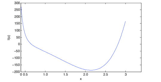
Figure 1. A plot of the integrand $I(u)$ with $u\mathop{\,{\scriptstyle\stackrel{{\scriptstyle\triangle}}{{=}}}}\,x$, $\bar{a}=2$, $R=-1000$, $\tau=\sqrt{72}$, $\sigma=\sqrt{48}$, $\rho=1/\pi$, and $\Omega=[0.4,3]$.

When the energy functional is convex, a weak solution can be found by minimizing the energy functional using a Newton-like iteration. However, when the energy is nonconvex, a weak solution may be a maximizer or saddlepoint of the energy. In this case, Newton’s method can be used to find a stationary point of the energy functional with progress towards a stationary point being guaranteed by computing steps along the Newton direction that yield sufficient decrease in a merit function. The positivity constraint $u>0$ can naturally be enforced when solving the Lichnerovich equation (2.1–2.3) using a safe-guarded Newton method. Unlike the Lichnerovich equation, the Yamabe Problem (1.1) does not have a singularity at $u=0$; thus, a barrier method can be used to help enforce the positive inequality constraint on $u$. In the following section, we consider barrier methods for nonconvex optimization and develop a primal barrier energy method for this class of problems.

3. Barrier methods for nonconvex optimization

Barrier methods are the most widely-used type of interior method for general nonlinear inequality-constrained optimization problems of the form:

$$\begin{array}[]{lc}{\displaystyle\mathop{\mathrm{minimize}}_{x\in\Re^{n}}}&f(x)\\ \hbox{\rm subject to}&c(x)\geq 0,\end{array}$$ (3.1)

where $f:\Re^{n}\rightarrow\Re$ is assumed to be twice-continuously differentiable and $c:\Re^{n}\rightarrow\Re^{m}$ is an $m$-vector of constraints. Generally speaking, barrier methods seek to minimize a composite function that both resembles the original function and naturally prevents infeasible iterates. Today, the most widely used barrier function is the classical logarithmic barrier function:

$$B_{\mu}(x)=f(x)-\mu\sum_{i=1}^{m}\ln c_{i}(x).$$ (3.2)

Notice that if $\mu$ is small, the barrier function resembles the original function; moreover, this function inherits the smoothness associated with the original problem but is only defined in the strict interior of the feasible region for the original problem (3.1).

The classical barrier method solves (3.1) by minimizing $B_{\mu}(x)$ for a decreasing sequence of positive $\mu$. Given a fixed $\mu>0$, first-order optimality conditions for $x^{*}$ to be a minimizer of the barrier function is that $\nabla B_{\mu}(x^{*})=0$, i.e.,

$$\nabla f(x^{*})-J(x^{*})^{T}y(x^{*})=0,$$ (3.3)

where $J$ denotes the constraint Jacobian and $y_{i}(x)\mathop{\,{\scriptstyle\stackrel{{\scriptstyle\triangle}}{{=}}}}\,\mu/c_{i}(x)$. Alternatively, $y$ is interpreted as a vector of Lagrange multipliers associated with the original inequality problem (3.1). Moreover, $c_{i}(x)y_{i}=\mu$ can be viewed a perturbation of the complementarity condition for a first-order KKT point.

When $c(x)\mathop{\,{\scriptstyle\stackrel{{\scriptstyle\triangle}}{{=}}}}\,x$, the Newton equations for minimizing $B_{\mu}(x)$ are given by

$$\left(\nabla^{2}f(x)+\mu\mathop{\mathrm{diag}}(X^{-2})\right)p=-\left[\nabla f(x)-\mu X^{-1}\right],$$ (3.4)

where $X^{-j}\mathop{\,{\scriptstyle\stackrel{{\scriptstyle\triangle}}{{=}}}}\,[1/x_{1}^{j},1/x_{2}^{j},\ldots,1/x_{n}^{j}]^{T}$ for $j\in\{1,2\}$, and $\mathop{\mathrm{diag}}(x)$ is the diagonal matrix whose $i$th diagonal entry is $x_{i}$. To ensure global convergence, a line search must be used to satisfy a sufficient decrease criteria (e.g., the Armijo or Wolfe conditions). Once a minimizer $x(\mu)$ of $B_{\mu}(x)$ is computed, $\mu$ is reduced and the process is repeated. Notice that the subsequent minimization can be warm-started by choosing the minimizer of the previous barrier function as the initial guess. Algorithm 3 summarizes the classical barrier method for solving (3.1) with $c(x)\mathop{\,{\scriptstyle\stackrel{{\scriptstyle\triangle}}{{=}}}}\,x$ and using the Amijo condition for sufficient descent.

                                                                                                                                   

Algorithm 3: Classical Barrier Method.

Choose $x_{0}>0$, $\mu>0$, $\eta\in\left(0,\frac{1}{2}\right)$, and $\gamma\in(0,1)$;

Set $k=0$;

while  $\mathop{\mathbf{not}\,}\mathit{converged}$  do 

Compute $x(\mu)$, an unconstrained minimizer of $B_{\mu}(x)$:

while  $\mathop{\mathbf{not}\,}\mathit{converged}$  do 

Solve (3.4) to obtain $p$;

Use the “99% rule” to compute $\alpha_{\max}$;

Compute $\alpha\in(0,\alpha_{\max}]$ such that $B_{\mu}(x+\alpha p)\leq B_{\mu}(x)+\eta\alpha\nabla B_{\mu}(x)^{T}p$;

$x\leftarrow x+\alpha p$;

end do

$x_{k+1}\leftarrow x(\mu)$;

$\mu\leftarrow\gamma\mu$;

$k\leftarrow k+1$;

end do

                                                                                                                                   

When computing a step length, it is necessary to safeguard the step to avoid taking a step into the infeasible region. For linear constraints, the so-called “99%” rule may be invoked (e.g., see  [6]) that states that if $\Delta x_{i}<0$ for at least one $i$: (i) Compute $\alpha_{max}=\max\{-(x_{i}/\Delta x_{i})\,\,:\,\,\Delta x_{i}<0\}$; (ii) Set the maximum step length to be $\bar{\alpha}=\max\{0.99\times\alpha_{max},1\}$.

We now state two theorems that summarize the convergence of the classical barrier method. The first theorem governs the local convergence of a sequence of minimizers of the classical barrier function. Before stating this theorem, we state the following theorem, which will be used in the proof of the theorem on local convergence.

Theorem 3.1.

Consider problem (3.1), where $f:\Re^{n}\rightarrow\Re$ and $c:\Re^{n}\rightarrow\Re^{m}$ are continuous. Let $\mathcal{N}$ denote the set of all local constrained minimizers with objective function value $f^{*}$, and assume that $f^{*}$ has been chosen so that $\mathcal{N}$ is nonempty. Assume further that the set $\mathcal{N}^{*}\subseteq\mathcal{N}$ is a nonempty compact isolated subset of $\mathcal{N}$. Then there exists a compact set $\mathcal{S}$ such that $\mathcal{N}^{*}$ lies in $\mathop{\mathrm{int}}(\mathcal{S})\cap\mathcal{F}$ and for any feasible point $\bar{x}$ in $\mathcal{S}$ but not in $\mathcal{N}^{*}$, $f(\bar{x})>f^{*}$. Furthermore, every point $x^{*}$ in $\mathcal{N}^{*}$ has the property that $f(x^{*})=f^{*}=\min f(x)$ for all $x\in\mathcal{S}\cap\mathcal{F}$.

Proof.

See [5, Theorem 7] and [12, Theorem 6]. ∎

The following theorem and proof regarding convergence of the minimizers of the barrier function is found in [6].

Theorem 3.2.

Consider problem (3.1), where $f:\Re^{n}\rightarrow\Re$ and $c:\Re^{n}\rightarrow\Re^{m}$ are continuous. Let $\mathcal{F}$ denote the feasible region, let $\mathcal{N}$ denote the set of minimizers with objective function value $f^{*}$, and assume that $\mathcal{N}$ is nonempty. Let $\{\mu_{k}\}$ be a strictly decreasing sequence of positive barrier parameters such that $\lim_{k\to\infty}\mu_{k}=0$. Assume that

1. there exists a nonempty compact set $\mathcal{N}^{*}$ of local minimizers that is an isolated subset of $\mathcal{N}$;

2. at least one point in $\mathcal{N}^{*}$ is in the closure of $\mathop{\mathrm{strict}}(\mathcal{F})$.

Then the following results hold:

1. there exists a compact set $\mathcal{S}$ such that $\mathcal{N}^{*}\subset\mathop{\mathrm{int}}(\mathcal{S})\cap\mathcal{F}$ and such that, for any feasible point $\bar{x}$ in $\mathcal{S}$ but not in $\mathcal{N}^{*}$, $f(\bar{x})>f^{*}$;

2. for all sufficiently small $\mu_{k}$, there is an unconstrained minimizer $y_{k}$ of the barrier function $B_{\mu_{k}}(x)$ in $\mathop{\mathrm{strict}}(\mathcal{F})\cap\mathop{\mathrm{int}}(\mathcal{S})$, with

   $$B_{\mu_{k}}(y_{k})=\hbox{\rm min}\,\{\,B_{\mu_{k}}(x)\mathop{\mathrm{:}}x\in\mathop{\mathrm{strict}}(\mathcal{F})\cap\mathcal{S}\,\}.$$

   Thus $B_{\mu_{k}}(y_{k})$ is the smallest value of $B_{\mu_{k}}(x)$ for any $x\in\mathop{\mathrm{strict}}(\mathcal{F})\cap\mathcal{S}$;

3. any sequence of these unconstrained minimizers $\{y_{k}\}$ of $B_{\mu_{k}}(x)$ has at least one convergent subsequence;

4. the limit point $x_{\infty}$ of any convergent subsequence $\{x_{k}\}$ of the unconstrained minimizers $\{y_{k}\}$ defined in (ii) lies in $\mathcal{N}^{*}$;

5. for the convergent subsequences $\{x_{k}\}$ of part (iv),

   $$\lim_{k\to\infty}f(x_{k})=f^{*}=\lim_{k\to\infty}B_{\mu_{k}}(x_{k}).$$

Proof.

See [6]. ∎

Applied to problem (3.1), the classical barrier method can be viewed as a path-following method that defines a path to both an optional $x^{*}$ and associated Lagrange multipliers $\lambda^{*}$.

The following theorem (stated and proved in [6] and based on results from [5, 12, 13]) summarizes the conditions under which a sequence of barrier minimizers converges to the solution of (3.1).

Theorem 3.3.

Consider problem (3.1). Assume that the set of strictly feasible points is nonempty. Let $x^{*}$ be a local constrained minimizer of (3.1), $\nabla f(x)\mathop{\,{\scriptstyle\stackrel{{\scriptstyle\triangle}}{{=}}}}\,g(x)$, $J(x)\mathop{\,{\scriptstyle\stackrel{{\scriptstyle\triangle}}{{=}}}}\,\nabla c(x)^{T}$, and $\mathcal{A}$ denote the set of indices of the active constraints at $x^{*}$. Assume that the following sufficient optimality conditions hold at $x^{*}$:

• $x^{*}$ is a KKT point, i.e., there exists a nonempty set $\mathcal{M_{\lambda}}$ of Lagrange multipliers $\lambda$ satisfying

  $$M_{\lambda}=\{\lambda\,:\,g(x^{*})=J(x^{*})^{T}\lambda,\,\,\lambda\geq 0,\,\,\text{and}\,\,c_{i}(x^{*})\lambda_{i}=0\,\,\,\forall i\};$$

• there exists $p$ such that $J_{\mathcal{A}}(x^{*})p>0$, where $J_{\mathcal{A}}(x^{*})$ denotes the active constraints at $x^{*}$; and

• there exists $\omega>0$ such that $p^{T}H(x^{*},\lambda)p\geq w\|p\|_{2}^{2}$ for all $\lambda\in\mathcal{M_{\lambda}}$ and all nonzero $p$ satisfying $g(x^{*})^{T}p=0$ and $J_{\mathcal{A}}(x^{*})p\geq 0$, where $H(x^{*},\lambda)\mathop{\,{\scriptstyle\stackrel{{\scriptstyle\triangle}}{{=}}}}\,\nabla^{2}f(x^{*})-\sum_{i=1}^{m}\lambda_{i}\nabla^{2}c_{i}(x^{*})$ is the Hessian of the Lagrangian evaluated at $x=x^{*}$.

Assume that a logarithmic barrier method is applied in which $\mu_{k}$ converges monotonically to zero as $k\rightarrow\infty$. Then

• there is at least one subsequence of unconstrained minimizers of the barrier function $B_{\mu_{k}}(x)$ converging to $x^{*}$;

• let $\{x^{k}\}$ denote such a convergent subsequence. Then the sequence of barrier multipliers $\{\lambda_{k}\}$, whose $i$th component is $\mu_{k}/c_{i}(x^{k})$ is bounded;

• $\lim_{k\rightarrow\infty}\lambda(x^{k})=\bar{\lambda}\in\mathcal{M_{\lambda}}$.

If, in addition, strict complementarity holds at $x^{*}$, i.e., there is a vector $\lambda\in\mathcal{M_{\lambda}}$ such that $\lambda_{i}>0$ for all $i\in\mathcal{A}$, then

• $\bar{\lambda}_{\mathcal{A}}>0;$

• for sufficiently large $k$, the Hessian matrix $\nabla^{2}B_{\mu_{k}}(x^{k})$ is positive definite;

• a unique, continuously differentiable vector function $x(\mu)$ of unconstrained minimizers of $B_{\mu}(x)$ exists for positive $\mu$ in a neighborhood of $\mu=0$; and

• $\lim_{\mu\rightarrow 0_{+}}x(\mu)=x^{*}$.

Proof.

See [6]. ∎

Consider the case when $c(x)\mathop{\,{\scriptstyle\stackrel{{\scriptstyle\triangle}}{{=}}}}\,x$, and the constrained local minimizer $x^{*}$ is strictly positive. In this case, Theorem 3.3 reduces to the following corollary:

Corollary 3.4.

Consider problem (3.1) with $c(x)\mathop{\,{\scriptstyle\stackrel{{\scriptstyle\triangle}}{{=}}}}\,x$. Suppose $x^{*}$ be a local constrained minimizer of (3.1). Further, assume that $x^{*}>0$. Let $\nabla f(x)$, $J(x)$ and $\mathcal{A}$ be defined as in Theorem 3.3. Assume that the following sufficient optimality conditions hold at $x^{*}$:

• $x^{*}$ is a stationary point of $f(x)$, i.e., $g(x^{*})=0$;

• $\nabla^{2}f(x^{*})$ is positive definite.

Assume that a logarithmic barrier method is applied in which $\mu_{k}$ converges monotonically to zero as $k\rightarrow\infty$. Then

• there is at least one subsequence of unconstrained minimizers of the barrier function $B_{\mu_{k}}(x)$ converging to $x^{*}$;

• let $\{x^{k}\}$ denote such a convergent subsequence. Then the sequence of barrier multipliers $\{\lambda(x^{k})\}$, whose $i$th component is $\mu_{k}/c_{i}(x^{k})$ is bounded;

• $\lim_{k\rightarrow\infty}\lambda(x^{k})=0$;

• for sufficiently large $k$, the Hessian matrix $\nabla^{2}B_{\mu_{k}}(x_{k})$ is positive definite;

• a unique, continuously differentiable vector function $x(\mu)$ of unconstrained minimizers of $B_{\mu}(x)$ exists for positive $\mu$ in a neighborhood of $\mu=0$; and

• $\lim_{\mu\rightarrow 0_{+}}x(\mu)=x^{*}$.

Proof.

This proof is based on the proof given in [6] for Theorem 3.3, modified for the case when $c(x)=x$ and the constrained local minimizer $x^{*}$ is strictly positive.

Since $x^{*}>0$, $x^{*}$ is in $\mathop{\mathrm{strict}}(\mathcal{F})$, and thus, in the closure of $\mathop{\mathrm{strict}}(\mathcal{F})$. Assumptions (a) and (b) imply that $x^{*}$ is an isolated unconstrained minimizer of $f(x)$. Thus, the conditions of Theorem 3.2 are met, implying that there is at least one subsequence of unconstrained minimizers of $B_{\mu_{k}}(x)$ converging to $x^{*}$. This proves (i).

Let $\{x^{k}\}$ denote such a convergent sequence, i.e., $\lim_{k\to\infty}x^{k}=x^{*}$. Each $x^{k}$ is an unconstrained minimizer of $B_{\mu_{k}}(x)$:

$$\nabla B_{\mu_{k}}(x)=g(x^{k})-\sum_{i=1}^{m}\nabla c_{i}(x^{k})\lambda_{i}(x^{k}),\quad\hbox{where}\quad\lambda_{i}(x^{k})=\frac{\mu_{k}}{c_{i}(x^{k})}.$$

Because $c(x^{k})>0$ (from Theorem 3.2, result (ii)), $\lambda_{i}(x^{k})$ is strictly positive for any $\mu_{k}>0$. Since there are no active constraints at $x^{*}$ and $x^{k}$ converges to $x^{*}$,

$$\lim_{k\to\infty}c_{i}(x^{k})=c_{i}(x^{*})>0,\quad\hbox{and hence}\quad\lim_{k\to\infty}\lambda_{i}(x^{k})=0,$$

for all $i=1,\ldots,m$, proving (ii) and (iii).

As in the proof of (v) in Theorem 3.3, to determine the properties of $\nabla^{2}B_{\mu_{k}}(x^{k})$ as $k\to\infty$, we write the Hessian of the barrier function (3.2) as

$$\nabla^{2}B_{\mu_{k}}(x^{k})=\nabla^{2}f(x^{k})+-\sum_{i=1}^{m}{\lambda_{i}(x^{k})}\;\nabla^{2}c_{i}(x^{k})+\sum_{i=1}^{m}\frac{\lambda_{i}(x^{k})}{c_{i}(x^{k})}\nabla c_{i}(x^{k})(\nabla c_{i}(x^{k}))^{T}.$$

Since $x^{k}\to x^{*}$ and $\lambda(x^{k})\to 0$ as $k\to\infty$, $\lim_{k\to\infty}\nabla^{2}B_{\mu_{k}}(x^{k})=\nabla^{2}f(x^{*})$. Thus, by assumption (b), for sufficiently large $k$, the Hessian $\nabla^{2}B_{\mu_{k}}(x^{k})$ is positive definite, proving (iv).

To verify the existence of a unique, differentiable function $x(\mu)$ for positive $\mu$ in a neighborhood of $x(\mu_{k})$, we apply the implicit function theorem (see, for example, [11, p. 128] and [10, pp. 585–586]) to the $n+1$ variables $(x,\mu)$. At $(x^{k},\mu_{k})$, we know that the following system of nonlinear equations has a solution:

$$\Phi(x,\mu)=g(x)$$

The Jacobian of $\Phi$ with respect to $x$ is the barrier Hessian $\nabla^{2}B_{\mu}(x)$, which was just shown to be positive definite at $x=x^{k}$ and $\mu=\mu_{k}$. The implicit function theorem then implies that there is a locally unique, differentiable function $x(\mu)$ passing through $x(\mu_{k})\mathop{\,{\scriptstyle\stackrel{{\scriptstyle\triangle}}{{=}}}}\,x^{k}$ such that $\Phi(x(\mu),\mu)=0$ for all positive $\mu$ in a neighborhood of $\mu_{k}$.

Using continuation arguments, it is straightforward to show that the function $x(\mu)$ exists for all $0<\mu\leq\mu_{k}$ for all sufficiently large $k$, giving result (vi).

Result (vi) is immediate from the local uniqueness of $x(\mu)$ and result (i), that $x_{k}$ is a local unconstrained minimizer of the barrier function. ∎

4. The Primal Barrier Energy Method

Inequality constraints on $u$ introduced in Section 2 can be enforced using a barrier method. Define

$$J_{\mu}(u)=J(u)-\mu\int_{\Omega}\ln(u)\,\,\,dx,$$

where $J(u)$ is defined as in (2.1). The Gateaux derivative is given by

$$J^{\prime}_{\mu}(u)(v) = J^{\prime}(u)(v)-\frac{d}{dt}\left[\mu\int_{\Omega}\ln(u+tv)\right]\bigg{|}_{t=0}$$ (4.1)

$$= \int_{\Omega}\left[\left(\bar{a}\nabla u\right)\cdot\nabla v+k(u)v\right]\,\,\,dx$$

$$+\int_{\partial_{N}\Omega}(cu-g_{N})v\,\,\,ds-\mu\int_{\Omega}u^{-1}v\,\,\,dx.$$

Thus, the condition for stationarity of $J_{\mu}(u)$ is given by solving the following problem:

$$\text{Find}~{}u\in H_{0}^{1}{(\Omega)}~{}\text{s.t.}~{}J^{\prime}_{\mu}(u)(v)=0,\ \ \forall v\in H_{0}^{1}{(\Omega)}.$$ (4.2)

The second Gateaux derivative of $J_{\mu}(u)$ is given by

$$J^{\prime\prime}_{\mu}(u)(w,v)=\int_{\Omega}\left[\left(\bar{a}\nabla w\right)\cdot\nabla v+k^{\prime}(u)wv\right]\,\,\,dx+\int_{\partial_{N}\Omega}cwv\,\,\,ds+\mu\int_{\Omega}u^{-2}wv\,\,\,dx.$$ (4.3)

Thus, the Newton update for solving (4.2) is given by:

$$\text{Find}~{}w\in H_{0,D}^{1}(\Omega)~{}\text{s.t.}~{}J^{\prime\prime}_{\mu}(u)(w,v)=-J^{\prime}_{\mu}(u)(v),\ \ \forall v\in H_{0,D}^{1}(\Omega).$$ (4.4)

4.1. Discretization

We use a standard Galerkin finite element method to approximate the solution (4.4) in an $N$-dimensional subspace $X_{h}\subset X=H_{0,D}^{1}(\Omega)\cap[u_{-},u_{+}]$. Thus, we seek a solution $u_{h}\in X_{h}$ such that

$$J^{\prime}_{\mu}(u_{h})(v_{h})=0,\ \ \forall v\in X_{h}.$$ (4.5)

The Newton update is given by:

$$\text{Find}~{}w_{h}\in X_{h}\subset X~{}\text{s.t.}~{}J^{\prime\prime}_{\mu}(u_{h})(w_{h},v_{h})=-J^{\prime}_{\mu}(u_{h})(v_{h}),\ \ \forall v_{h}\in X_{h}.$$ (4.6)

Let $\{\phi_{i}\}_{1}^{N}$ be a basis $X_{h}$. Then, without loss of generality, let

$$u_{h}=\sum_{i}^{N}\alpha_{i}\phi_{i},\quad w_{h}=\sum_{i}^{N}\beta_{i}\phi_{i},$$

for some $\{\alpha_{i}\}$ and $\{\beta_{i}\}$. It is sufficient to take the test functions $v_{h}\in X_{h}$ to be the basis functions $\{\phi_{i}\}_{i=1}^{N}$. Equation (4.6) is equivalent to solving the following matrix-vector equation:

$$\left[A(u_{h})+\mu M(u_{h})\right]W=-\left[G(u_{h})-\mu H(u_{h})\right],$$ (4.7)

where

$$A_{ij}(u_{h}) = J^{\prime\prime}_{\mu}(u_{h})\left(\phi_{j},\phi_{i}\right),$$ (4.8)

$$M_{ij}(u_{h}) = \int_{\Omega}\left(u_{h}\right)^{-2}\phi_{j}\phi_{i}\,\,\,dx$$ (4.9)

$$W_{i} = \beta_{i},$$ (4.10)

$$G_{i}(u_{h}) = J^{\prime}_{\mu}(u_{h})(\phi_{i}),$$ (4.11)

$$H_{i}(u_{h}) = \int_{\Omega}(u_{h})^{-1}\phi_{i}\,\,\,dx$$ (4.12)

The barrier term contributes an extra term to the system matrix, namely

$$M=\mu\int_{\Omega}u_{h}^{-2}\phi_{j}\phi_{i}\,\,\,dx.$$

Thus, the barrier term adds a positive definite matrix to the original system matrix, and so, may be viewed as a regularization. In FETK, this integral is approximated using a high-accuracy quadrature rule, using a finite sum with fixed positive weights.

The Newton update $W$ defines a descent direction for

$$\phi(u_{h})=\frac{1}{2}\|G(u_{h})\|_{2}^{2},$$ (4.13)

and thus, $\phi(u_{h})$ may be used as a merit function to enforce sufficient descent.

At optimality, the solution $u_{h}$ must lie in the strict interior of the feasible region, and thus, the Lagrange multipliers must be exactly zero. Because of this, there is no restriction that $\mu$ must be kept away from zero. Thus, $\mu$ may be steadily decreased, and in fact, may be set to zero–solving the original stationary problem.

Algorithm 4.1 summarizes the primal barrier energy method:

                                                                                                                                   

Algorithm 4.1: Primal Barrier Energy Method.

Choose $u_{0}>0$, $\mu>0$, $\eta\in\left(0,\frac{1}{2}\right)$, and $\gamma\in(0,1)$;

Set $k=0$;

while  $\mathop{\mathbf{not}\,}\mathit{converged}$  do 

Compute $u(\mu)$ to approximately solve (4.5):

while  $\mathop{\mathbf{not}\,}\mathit{converged}$  do 

Solve (4.7) to obtain $w^{i}_{h}$;

Use the “99% rule” to compute $\alpha_{\max}$;

Compute $\alpha\in(0,\alpha_{max}]$ such that $\phi(u^{i}_{h}+\alpha w^{i}_{h})\leq\phi(u^{i}_{h})+\eta\alpha\nabla\phi(u_{h}^{i})^{T}w^{i}_{h}$;

$u^{i}_{h}\leftarrow u^{i}_{h}+\alpha w^{i}_{h}$;

end do

$u_{k+1}\leftarrow u(\mu)$;

$\mu\leftarrow\gamma\mu$;

$k\leftarrow k+1$;

$i\leftarrow 0$;

end do

                                                                                                                                   

In practice, each barrier function $B_{\mu}(x)$ does not have to be minimized to high precision. Typically, each barrier function is considered sufficiently minimized when the norm of its gradient is either less than an fixed absolute tolerance or satisfies a relative tolerance based on $B_{\mu}(x_{0})$, where $x_{0}$ denotes the initial guess for the minimization (see, for example, [4]).

5. Numerical Results

The standard Newton method, a standard Newton method with safeguarding, and the primal barrier energy method was implemented using FETK (the Finite Element ToolKit; see [7] and http://www.FETK.org). These methods were used to solve the Einstein constraint equations on three single-hole domains, centered at the origin, with given boundary conditions on both the inner and outer boundary. Each tetrahedral mesh was generated by the GAMer component of FETK, which is a high-fidelity surface and volume meshing tool based on standard simplex triangulation, subdivision, and smoothing algorithms (cf. [14, 15]). Details of the three meshes are given in Table 1.

Table 1. Meshes

	Mesh #1	Mesh #2	Mesh #3
Inner radius	50	10	1
Outer radius	100	100	100
Vertices	2089	1436	2820
Simplicies	9726	7589	15321

At the heart of each nonlinear solver is a linear solver (e.g., sparse direct solver or the conjugate-gradient (CG) method). For more ill-conditioned systems, the Newton equations may not be solved exactly; however, it is necessary that any step obtained from the linear solver of choice must be a descent direction. A simple backtracking line search is used to obtain a step that meets the sufficient decrease criteria in Algorithms 3 and 4.1. Convergence is obtained when the norm of the nonlinear residual defining the PDE is less than a chosen tolerance of $\epsilon\mathop{\,{\scriptstyle\stackrel{{\scriptstyle\triangle}}{{=}}}}\,$1.0e-07, i.e.,

$$\|G(u_{k})\|_{2}\leq\epsilon.$$ (5.1)

For each example, the energy barrier method initialized $\mu$ and then decreased $\mu$ whenever the iterate $u^{k}_{h}$ satisfied

$$\|f(u^{k}_{h})\|_{2}\leq\max\{\epsilon_{\mu}\|f(u^{0}_{h})\|_{2},\epsilon_{\mu}\}$$ (5.2)

where $f(u^{k}_{h})=G(u^{k}_{h})-\mu H(u^{k}_{h})$, $u^{0}_{h}$ denotes the initial iterate after decreasing $\mu$, and $\epsilon_{\mu}=\max\{\min\{0.1,\mu\},\epsilon\}$. This choice of $\epsilon_{\mu}$ allows each subproblem to be solved to greater accuracy as $\mu$ is decreased.

Reasonable choices for parameters for the Lichnerov equation with boundary conditions include those given in Examples 1–2, in Section 2.2. The first two examples are with these choices of parameters.

Example 1. Set $\bar{a}=1.0$, $R=1.0$, $\tau=0.1$, $\sigma=0.2$, $\rho=0.1$, $c=1.0$, and $g_{N}=-1.0$. We pick $\Omega$ to have Robin boundary conditions on both the inner and outer boundary. The presence of the negative exponents acts as a natural barrier function, preventing infeasible iterates. For this reason, to obtain a positive solution it is sufficient to add a safeguarding procedure such as the so-called “99% rule” (see Section 3) to the standard Newton method.

Table 2 gives the results of using the standard Newton method, Newton’s method with safeguarding using the “99% rule”, and the primal energy method to solve the Lichnerovich equation. For each solver, the initial guess was a vector of all ones. We list the number of iterations (“itns”), residual, and the signs of the entries in the vector of coefficients for $u_{h}$ (i.e., $+$ denotes all the entries are strictly positive, $-$ denotes all the entries are strictly negative, and $+/-$ denotes both positive and negative entries). Note that there is one linear solve per iteration, and thus, the number of iterations is also the number of linear solves required by each method. All four solvers converged on all three meshes to strictly positive solutions.

In Table 2, the energy barrier method is reported with two different initial values of $\mu$. First, the energy barrier method was run with $\mu=0.0$, making it numerically equivalent to Newton’s method with safeguarding. (For nonconvex problems, we do not expect the energy barrier method to converge to a strictly positive solution with this choice of $\mu$). For illustrative purposes, the results with $\mu=1.0$ are also reported; for this test, when each subproblem was sufficiently solved (i.e., (5.2) was satisfied), we reduced $\mu$ by a factor of $1/10$. However, for this convex problem, allowing faster reductions of $\mu$ leads to fewer overall iterations. In fact, reducing $\mu$ by a factor of $1/100$ led to 14 iterations on mesh #1, 16 iterations on mesh #2, and 16 iterations on mesh #3. For more difficult problems, reducing $\mu$ too quickly will impede convergence. Even though faster reductions in $\mu$ would lead to results more similar to the Newton methods, for the results in Table 2, we chose to display results with a reasonable, commonly accepted reduction of $1/10$. Also, it is worth noting that the different residual values for the algorithms are inconsequential in that convergence only requires (5.1) to be satisfied. (In these cases, Newton’s method was fortunate in that quadratic convergence led to a much smaller residual for each final iterate.)

In Table 2 we see that a positive solution was obtained by all methods using an initial guess of all ones. As previously noted, a barrier method is not required to obtain a strictly positive solution since the energy functional has a natural barrier in the form of negative coefficients of $u$. Thus, we expect that a safeguarded Newton method will be sufficient to recover a positive solution. In this example, Newton’s method with and without safeguarding produced the same iterates. It is of interest to note that a strictly negative solution can be recovered on all three meshes by using the standard Newton method together with the initial guess of a vector of all negative ones.

Table 2. Example #1.

	Mesh #1			Mesh #2			Mesh #3
method	itns	resid	sign	itns	resid	sign	itns	resid	sign
Newton (standard)	6	2.71e-12	+	6	5.15e-12	+	6	4.73e-12	+
Newton (safeguarded)	6	2.71e-12	+	6	5.15e-12	+	6	4.73e-12	+
Barrier energy ($\mu_{0}=0.0$)	6	2.71e-12	+	6	5.15e-12	+	6	4.73e-12	+
Barrier energy ($\mu_{0}=1.0$)	22	6.15e-08	+	24	1.19e-08	+	24	1.17e-08	+

Example 2. Let $a=2$, $R=-1000$, $\tau=\sqrt{72}$, $\sigma=\sqrt{48}$, and $\rho=1/\pi$. For this example, the inner and outer boundaries of all three meshes have a Robin boundary condition with $c=2$ and $g_{N}=10$.

On the first mesh, the standard Newton method failed to converge in 50 iterations, denoted by the asterisk in Table 3; in fact, at the 100th iteration, the current approximation to $u_{h}$ contained both positive and negative entries–the standard Newton method was unable to maintain a strictly positive solution. When the initial guess was set to a vector whose entries were all 10, Newton’s method converged to a positive solution; when the initial guess was set to a vector whose entries were all -10, the standard Newton method returned a strictly negative solution; and when the initial guess was set to a vector whose enries were all -1, the standard Newton method returned a strictly positive solution. (Newton’s method without safeguarding was unpredictable–one could recover a positive solution even when starting with an initial negative guess.) Meanwhile, with an initial guess of all ones, the safeguarded Newton method converged to a strictly positive solution. The barrier energy method converged with $\mu_{0}=1$ and subsequent reductions in $\mu$ of $1/10$, as in Example 1.

On the second mesh, all methods converged to the same strictly positive solution when the initial guess was all ones. (The barrier energy method was run with $\mu_{0}=1$ and subsequent reductions in $\mu$ of $1/10$, as in Example 1.) A strictly negative solution can be recovered by using the standard Newton method together with the initial guess of a vector whose entries are all -10.

On the third mesh, Newton’s method without safeguarding did not converge within the first 100 iterations and had both positive and negative components. A negative solution was obtained by the standard Newton method by starting with a vector whose entries were all -10. Meanwhile, Newton’s method with safeguarding made insignificant progress after the seventh iteration, and thus, failed to converge in 100 iterations. The safeguarded method failed because the initial safeguarded Newton steps took some of the coefficients of $u_{h}$ very close to the boundary and the following Newton directions continued to point in the direction of negative numbers for these components. In this event, the “99% rule” allows subsequent steps of only negligible size along the Newton direction at each iteration. As a result, the safeguarded Newton method is unable to make any real progress each subsequent iteration, and thus, fails to converge.

In this example, we see that even though there is a natural barrier in the Lichnerovich equation, there are additional benefits that a barrier function approach can offer: By setting the parameter $\mu$ to be large enough, we can alter the pure Newton direction, preventing the initial Newton iterates from getting too close to the boundary. For example, setting $\mu_{0}$ to be 10, 20, 30, or 40, the energy method’s iterates took large initial steps to the boundary, preventing convergence; however, with $\mu_{0}=50$, the algorithm converged to a positive solution. (The values in Table 3 are with $\mu_{0}=50$ and subsequent reductions in $\mu$ of $1/10$.)

The energy barrier method was the only method to find a strictly positive solution to this problem on all three meshes.

Table 3. Example #2.

	Mesh #1			Mesh #2			Mesh #3
method	itns	resid	sign	itns	resid	sign	itns	resid	sign
Newton (standard)	*	4.69e+19	+/-	11	9.80e-08	+/-	*	4.92e+20	+/-
Newton (safeguarded)	9	2.89e-09	+	7	1.37e-08	+	*	2.01e+07	+
Barrier energy	16	4.02e-08	+	16	7.67e-08	+	17	9.47e-09	+

Example 3. Consider following Yamabe problem:

$$-8\Delta u+\rho(r)u^{5}=0,$$

where $\rho(r)=1/r^{3}$, and $r$ is the Euclidean distance. (This choice of $\rho(r)$ was motivated by equation (41) in [1]). For this example, we impose the Dirichlet condition $u=1$ on both the inner and outer boundaries of all three meshes. For this example, the initial guess was taken to be a vector of ones; given the Dirichlet condition, this is a reasonable starting point.

Table 4 reports the results of each solver on this problem. Neither backtracking nor a barrier method was required to solve this problem.

Table 4. Example #3.

	Mesh #1			Mesh #2			Mesh #3
method	itns	resid	sign	itns	resid	sign	itns	resid	sign
Newton (standard)	1	1.91e-08	+	2	1.16e-12	+	3	1.18e-12	+
Newton (safeguarded)	1	1.91e-08	+	2	1.16e-12	+	3	1.18e-12	+
Barrier energy ($\mu$=1.0)	18	1.13e-12	+	22	1.25e-12	+	23	1.34e-12	+

Example 4. For this example, we modify the problem in Example 3 to include the extra term in (1.1):

$$-8\Delta u-\frac{1}{8}u=-\rho(r)u^{5},$$

where $\rho(r)=1/r^{3}$, and $r$ is the Euclidean distance. Also, assume Dirichlet boundary conditions of $u=1$ on both the inner and outer boundaries. For this example, the initial guess was taken to be a vector of ones.

Table 5 contains the results on all three meshes. The standard Newton method converged quickly to a solution with positive and negative components on each mesh. Newton’s method with safeguarding did not converge on any mesh. On the all three meshes, the method took initial large steps to the boundary and made negligible progress after ten iterations. The primal barrier energy method with $\mu_{0}=1$ converged on the first mesh, but this initial value of $\mu$ on the second mesh was too small. With $\mu_{0}=10$, the primal barrier energy method converged to a strictly positive solution on all three meshes.

Table 5. Example #4.

	Mesh #1			Mesh #2			Mesh #3
method	itns	resid	sign	itns	resid	sign	itns	resid	sign
Newton (standard)	11	2.71e-08	+/-	16	9.65e-09	+/-	18	8.97e-11	+/-
Newton (safeguarded)	*	9.16e+03	+	*	1.64e+04	+	*	1.47e+04	+
Barrier energy ($\mu$=10.0)	17	1.94e-11	+	18	2.86e-11	+	18	2.69e-11	+

6. Conclusion

In this article we considered both the design and the analysis of a certain class of nonconvex optimization-based numerical methods for approximating positive solutions to nonlinear geometric elliptic partial differential equations containing critical exponents. As noted, these types of problems arise regularly in geometric analysis and mathematical physics; our primary interest here was Yamabe problem and the Einstein constraint equations. The difficulty one faces with these problems are the simultaneous presence of several challenging features, including spatial dimension $n\geqslant 3$, varying and potentially non-smooth coefficients, critical (or even super-critical) nonlinearity, non-monotone nonlinearity (arising from a non-convex energy), and spatial domains that are typically Riemannian manifolds rather than simply open sets in $R^{n}$. For these types of problems, there may be multiple solutions, although only positive solutions typically have mathematical and physical meaning. This creates additional complexities in both the theory and numerical treatment of such problems, as this feature introduces both non-uniqueness as well as the need to incorporate an inequality constraint into the formulation. As a practical approach for treating these difficulties, we considered numerical methods based on Galerkin-type discretization, covering any standard bases construction (finite element, spectral, or wavelet), and the combination of a barrier method for nonconvex optimization and global inexact Newton-type methods for dealing with nonconvexity and the presence of inequality constraints. After giving an overview of barrier methods in non-convex optimization, we then developed and analyzed a primal barrier energy method. We then presented a sequence of numerical experiments using this type of barrier method, based on a particular Galerkin method, namely the piecewise linear finite element method, leverage the FETK modeling package. In the experiments, the negative pole in the Hamilitonian constraint provided a “natural” barrier, aiding the convergence of Newton methods. In this setting, a barrier method will often be unnecessary; however, in some cases the numerical experiments showed that allowing for a flexible barrier parameter can be helpful (see Example 2, Mesh #3). The experiments also confirmed that on some classes of Yamabe problems, a solution could not be found without the use of a barrier method (see Example #4), suggesting that barrier methods are more useful on critical exponent problems without singularities that arise from lower-order negative exponent terms.

Although we considered here only scalar elliptic equations with variational structure, that is, they that arise as the Euler condition for stationarity of an underlying (usually nonconvex) energy, more generally these types of critical exponent problems may arise as part of a more complex elliptic system. A prime example is the coupled Hamiltonian and momentum constraints in the Einstein equations [8, 9]. While the Hamiltonian constraint (as well as the momentum constraint) alone has variational structure, when combined as a system there is in fact no variational structure to exploit. Nevertheless, the ideas in this paper can be applied by using alternative formulations of the Einstein constraints, and will be pursued in a second article.

References

- [1] T. W. Baumgarte, N. O. Murchadha, and H. P. Pfeiffer. Einstein constraints: Uniqueness and nonuniqueness in the conformal thin sandwich approach. Phys. Rev. D, 75(4):044009, Feb 2007.
- [2] C. Budd. Weak finite-dimensional approximations of semi-linear elliptic pdes with near-critical exponents. Asymptotic Analysis, 17(3):185–220, 1998.
- [3] C. Budd and A. Humphries. Adaptive methods for semi-linear elliptic equations with critical exponents and interior singularities. Applied Numerical Mathematics, 26(1):227–240, 1998.
- [4] R. S. Dembo, S. C. Eisenstat, and T. Steihaug. Inexact Newton methods. SIAM J. Numer. Anal., 19(2):400–408, 1982.
- [5] A. V. Fiacco and G. P. McCormick. Nonlinear Programming. Classics in Applied Mathematics. Society for Industrial and Applied Mathematics (SIAM), Philadelphia, PA, second edition, 1990. Reprint of the 1968 original.
- [6] A. Forsgren, P. E. Gill, and M. H. Wright. Interior methods for nonlinear optimization. SIAM Rev., 44:525–597, 2002.
- [7] M. Holst. Adaptive numerical treatment of elliptic systems on manifolds. Advances in Computational Mathematics, 15(1–4):139–191, 2001. Available as arXiv:1001.1367 [math.NA].
- [8] M. Holst, G. Nagy, and G. Tsogtgerel. Far-from-constant mean curvature solutions of Einstein’s constraint equations with positive Yamabe metrics. Physical Review Letters, 100(16):161101.1–161101.4, 2008. Available as arXiv:0802.1031 [gr-qc].
- [9] M. Holst, G. Nagy, and G. Tsogtgerel. Rough solutions of the Einstein constraints on closed manifolds without near-CMC conditions. Comm. Math. Phys., 288(2):547–613, 2009. Available as arXiv:0712.0798 [gr-qc].
- [10] J. Nocedal and S. J. Wright. Numerical Optimization. Springer-Verlag, New York, 1999.
- [11] J. M. Ortega and W. C. Rheinboldt. Iterative solution of nonlinear equations in several variables. Society for Industrial and Applied Mathematics (SIAM), Philadelphia, PA, 2000. Reprint of the 1970 original.
- [12] M. H. Wright. Interior methods for constrained optimization. In Acta Numerica, 1992, pages 341–407. Cambridge University Press, New York, USA, 1992.
- [13] S. J. Wright and D. Orban. Properties of the log-barrier function on degenerate nonlinear programs. Preprint ANL/MCS-P772-0799, Mathematics and Computer Science Division, Argonne National Laboratory, Argonne, IL, July 1999.
- [14] Z. Yu, M. Holst, Y. Cheng, and J. McCammon. Feature-preserving adaptive mesh generation for molecular shape modeling and simulation. Journal of Molecular Graphics and Modeling, 26:1370–1380, 2008.
- [15] Z. Yu, M. Holst, and J. McCammon. High-fidelity geometric modeling for biomedical applications. Finite Elem. Anal. Des., 44(11):715–723, 2008.