Statistical analysis of structural transitions in small systems

Abstract

We discuss general thermodynamic properties of molecular structure formation processes like protein folding by means of simplified, coarse-grained models. The conformational transitions accompanying these processes exhibit similarities to thermodynamic phase transitions, but also significant differences as the systems that we investigate here are very small. The usefulness of a microcanonical statistical analysis of these transitions in comparison with a canonical interpretation is emphasized. The results are obtained by employing sophisticated generalized-ensemble Markov-chain Monte Carlo methodologies.

1 Polymers and proteins

In heterogeneous many-particle systems, where typically different energy scales, associated with the inter-particle interactions, compete with each other, the formation of stable composites is a complex process. This is even more relevant if the many-particle system exhibits constraints such as covalent chemical bonds restricting the mobility of atomistic or monomeric subunits. Furthermore, the flexibility of the molecular system to adapt to environmental conditions (solvent, temperature, pressure, etc.) is reduced. Non-covalent interactions among such subunits which are due, for example, to dipole–dipole interactions (van der Waals “bonds”, hydrogen bonds), cause additional limitations [1].

Concentrating on linear, linelike molecules in solvent, two major classes are discriminated: homopolymers and heteropolymers. Homopolymers are chains of repeated identical subunits, i.e., chemical groups (“monomers”); a typical example is polyethylene -[CH₂]-. The “two ends” of the backbone of the characteristic monomers (in the case of polyethylene this is the methylene group CH₂) are connected by covalent bonds (e.g., C-C) with the previous and the next group, respectively.

In general, depending on symmetry and stability, covalent bonds strongly differ in their response to excitations, which, for example, can be induced by external fields or thermal fluctuations. If, under present environmental conditions and external fields, these bonds are hardly excited to perform fluctuations, then they are rather “stiff”, i.e., the contour length of the chain is widely conserved. Thus, depending on the backbone stiffness, longitudinal degrees of freedom are frozen and thus result in constraints of the tangential monomeric mobility. In other cases, polymers can be elastic and due to the longitudinal flexibility, the contour length fluctuates upon excitation.

Basic backbone geometries that can be associated with such linelike objects are helices, strands, rodlike, and “random” wormlike conformations. Helices and sheets belong to the class of secondary structures and are stabilized by hydrogen bonds formed by dipole–dipole interactions of polar groups (e.g., -CO, -NH, -OH) in the polymer backbone. However, it shcould be noted that the formation of hydrogen bonds is not a necessary condition for the onset of secondary structures which are rather elementary intrinsic geometries of such linear monomeric chains. This is particularly visible, if the monomers contain side chains whihc can be modeled as tubelike polymers [2, 3].

If the monomers have a larger chemical complexity, e.g., by the existence of side chains (e.g., polar groups, aromatic rings, etc.) protruding from the backbone, repulsive volume exclusion effects and attractive interactions among side chains (caused by electrostatic, van der Waals, or hydrophobic forces), higher-order (“tertiary”), i.e., crystalline or amorphous, glassy structures can form. These interactions entail a further, not necessarily uniform, limitation of the individual monomeric mobility. Typically, the energy of such non-covalent bonds among side chains of different monomers is typically sufficiently small and non-covalent bonds can break by comparatively weak changes of environmental conditions. Consequently, different phases of polymers are discriminated which depend on temperature, polymer concentration, solvent quality, pressure, presence of external fields, etc.

However, despite the huge number of natural and technologically important synthesized polymers with different chemical composition, a rough classification of linear polymers into groups of flexible, semiflexible, and stiff polymers is possible. Thus, only a few system parameters, based on the fundamental length and energy scales associated with covalent bonds and non-covalent interactions, are necessary to describe the generic phase behavior of classes of polymers [1]. Conformational transitions of single homopolymers can be understood as thermodynamic phase transitions if the degree of polymerization, i.e., the length of the chain or the number of monomers $N$, is huge [4, 5]. The general structural behavior of polymers is typically described by geometric quantities such as the end-to-end distance $R_{\rm ee}$ and the radius of gyration $R_{\rm gyr}$, the latter being a measure for the compactness of polymers. For very long chains, i.e., in the limit $N\to\infty$, the ensemble average has a power-law form, $\langle R_{\rm ee,gyr}^{2}\rangle\sim N^{2\nu}$, where $\nu$ is a universal exponent which is a characteristic constant in the structural phase the polymer resides in. For a flexible interacting polymer in good solvent (or temperatures $T$ above the $\Theta$ point $T_{\Theta}$), for example, $\nu\approx 3/5$. This corresponds to the behavior of self-avoiding walks (random coils with pure steric volume exclusion). At the $\Theta$ point that separates good from poor solvent conditions, or alternatively, the random-coil phase from the globular phase of compact conformations at $T_{\Theta}$, $\nu=1/2$. The polymer behaves like a random walk – repulsive volume exclusion and attractive monomer–monomer interaction cancel each other. In the globular and crystalline phase ($T<T_{\Theta}$), very compact (or spherical) conformations dominate and thus $\nu\approx 1/3$.

However, it should be noted that the interest in polymers of rather small length $N\ll\infty$ has increased in the past years with the onset of nowadays available high-resolution experimental techniques and the demand for nanofabrication of molecular applications. The investigation of the finite-length behavior of single polymers sheds some new light on the conformational transitions of polymers. Nucleation effects are governed by the competition of likewise surface and volume effects as well as entropic ambiguity and energetic significance of polymer conformations in a certain macrostate (“pseudophase”) and close to transitions between different macrostates (“pseudophase transitions”). The thermodynamic limit is not of relevance anymore and thus also is not the asymptotic critical behavior. The understanding of subphases and transitions in-between becomes crucial, but this is challenging because of the high specificity of small polymers. Thus, a generic classification of conformational subphases is an intricate problem as details of monomeric properties – even down to the atomistic level – can essentially influence the overall pseudophase behavior. The description of structural behavior by means of theoretical models is, therefore, difficult and one has to be aware that results of studies of the same polymer can differ from model to model. Thus, model studies of finite-length polymers are of highly qualitative nature and results have to be interpreted as “possible scenarios” rather than definite answers [6].

This is particularly relevant for a special class of polymers, the heteropolymers. The most prominent representatives are the proteins which are the workhorses in all biological cell systems. Proteins are synthesized by the ribosomes in the cell, where the genetic code in the DNA is translated into a sequence of amino acids. The folding of a synthesized protein into its three-dimensional structure is typically a spontaneous process that takes place in an aqueous environment. In a complex biological system, the large variety of processes which are necessary to keep an organism alive requires an ensemble of different functional proteins. In the human body, for example, about 100 000 different proteins fulfill specific functions. However, this number is extremely small, compared to the huge number of possible amino acid sequences ($=20^{N}$, where $N$ is the number of amino acids, typically in the range 100 to 3000). The reason is that bioproteins have to obey very specific demands. Most important are stability, uniqueness, and functionality.

2 Folding transitions of proteins

The structural changes a protein experiences in the folding process are of different nature. There are rather local, but nonetheless cooperative arrangements of monomeric subunits in helical or sheetlike segments. These are secondary structures (the amino acid sequence is the primary structure). The formation of secondary structures is a conformational transition; a very prominent one is the helix-coil transition: In a collective effect of orientational ordering, an unfolded segment of adjacent amino acids transforms into a helical substructure. Molecular helix-coil transitions are typically accompanied by hydrogen-bond formation. Hydrogen bonds stabilize the symmetry of secondary structures. A famous example is the Watson-Crick $\alpha$-helix with 3.6 amino acids per winding (see Fig. 1).

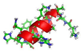
Figure 1: The C-peptide of ribonuclease A consists of 13 amino acids and is a typical $\alpha$-helix former.

In proteins, the size of individual secondary-structure segments is typically rather small. The reason is that proteins are “interacting polymers”, i.e., the amino acids strongly interact with each other and form a globular or tertiary shape. This is due to the fact that amino acids possess a uniform backbone and differ only in their side chains. Adjacent amino acid backbones are connected via the peptide bond and electric dipoles formed by backbone atoms are typically involved in hydrogen-bond formation. Backbone-backbone interaction provides the symmetry of secondary structures. However, the interaction between the non-bonded side chains is non-uniform and strongly dependent of the side chain type. Roughly, two significantly different classes of side chains occur: hydrophilic ones that favor contact with a surrounding polar solvent like water and hydrophobic side chains which are non-polar, thus disfavoring contact with water molecules (for representatives of the two classes see Fig. 2). Therefore, the effective force that leads to the formation of a compact hydrophobic core surrounded by a screening shell of polar amino acids is called hydrophobic force. For spontaneously folding single-domain proteins it is the essential driving force in the tertiary folding process.

The folded structure of a functional bioprotein is thermodynamically stable under physiological conditions, i.e., thermal fluctuations do not lead to significant globular conformational changes. To force tertiary unfolding requires an activation energy that is much larger than the energy of the thermal fluctuations. This activation barrier can be drastically reduced by the influence of other proteins, the prions. The Creutzfeld-Jakob disease is an example for the disastrous consequences prion-mediated degeneration of proteins can cause in the brain. The folded structure and the statistical ensemble of native-like structures, which are morphologically identical to the native fold, form a macrostate. It represents a conformational phase which is energy-dominated. Functionality of the native structure is only assured if entropic effects are of little relevance.

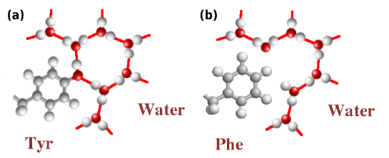
Figure 2: (a) Tyrosine (Tyr) is an amino acid with an OH group in the side chain. Thus, it is hydrophilic as the OH dipole can form a hydrogen bond with a polar solvent molecule (water). (b) Phenylalanine (Phe), on the other hand, is a typical example for a hydrophobic amino acid. The CH₂-C₆H₅ side chain does not contain a polar group. Phe in the surface-accessible protein shell would disturb the hydrogen-bond network of the solvent which is energetically disfavored.

A significant change of the environmental conditions such as temperature, pH value, or, following the above example, the prion concentration, can destabilize the folded phase. Entropy becomes relevant, the entropic contribution to the free energy starts dominating over energy. Consequently, the hydrophobic core decays. This does not necessarily lead to a globular unfolding of the protein. A rather compact intermediate conformational phase can be stable [7]. However, further imbalancing the conditions will finally lead to the phase of randomly unstructured coils. The latter transition is often called “folding/unfolding transition”, whereas the hydrophobic core formation is referred to as “glassy transition”, as unresolvable competing energetic effects may result in frustration. The primary structure, i.e., the sequence of different amino acids lining up in proteins, is already sort of quenched disorder.

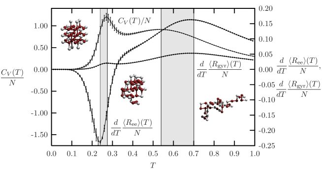
Figure 3: Folding thermodynamics of a 42-residue peptide using a simple hydrophobic-polar lattice peptide model [9]. Shown are the specific heat and fluctuations of structural quantities such as end-to-end distance and radius of gyration.

A simple example for these transitions accompanying a lattice peptide [8] folding process is shown in Fig. 3, where the specific heat $C_{V}$ and the fluctuations of end-to-end distance and radius of gyration, $d\langle R_{\rm ee,gyr}\rangle/dT$, are plotted as functions of temperature. Above the folding transition, structureless conformations dominate the “vapor phase”. Below the folding transition, but above the hydrophobic-core collapse, very compact “globular” structures form the “liquid phase”. When, for lower temperatures, the hydrophobic-core formation proceeds, the fluctuations get smaller. Finally, the native state with maximally compact hydrophobic core has formed. As in this example, the native state is not necessarily the overall most compact conformation. This is obvious from the negativity of the gyration radius fluctuations in this transition region. Although all fluctuating quantities clearly signalize the transitions, the peak temperatures do not perfectly coincide. This is a typical indication for the finiteness of the system. There are no transition points in protein structure-formation processes, but rather transition regions [6, 9]. This separates conformational transitions of finite-length polymers (pseudophase transitions) from thermodynamic phase transitions being considered in the thermodynamic limit.

3 Microcanonical vs. canonical interpretation

The smallness of such systems can cause surprising side-effects in nucleation processes which protein folding belongs to. Since the formation of the solvent-accessible hydrophilic surface and the bulky hydrophobic core is crucial for the whole tertiary folding process, the competition between surface and volume effects significantly influences the thermodynamics of nucleation [10, 11, 12, 13, 14]. For this reason, it is not obvious at all, which statistical ensemble represents the appropriate frame for the thermodynamic analysis of folding processes. This is even more intricate, as one may think. It is, for example, quite common to interpret phase transitions by means of fluctuating quantities calculated within the canonical formalism. Transition points are characterized by divergences in the fluctuations (second-order phase transitions) or entropy discontinuities (first-order transitions), occurring at unique transition temperatures. This standard analysis is based on the assumption that the temperature is a well-defined quantity, as it seems to be an easily accessible control parameter in experiments. This assumption is true for very large systems ($N\to\infty$) with vanishing surface/volume ratio in equilibrium, where surface fluctuations are irrelevant. The microcanonical Hertz entropy $S(E)=\ln\,G(E)$ (with $k_{B}=1$ in our units), where $G(E)=\int_{E_{\rm min}}^{E}dE^{\prime}g(E^{\prime})$ is the integrated density of states, is a concave function and thus the microcanonical temperature, defined by the mapping ${\cal F}:E\mapsto T=:T(E)=[\partial S(E)/\partial E]^{-1}$, never decreases with increasing energy $E$. A discrimination of the parameter “temperature” in the canonical ensemble and the microcanonical (caloric) temperature $T(E)$ is not necessary, as energetic fluctuations vanish and thus the canonical and the microcanonical ensemble are equivalent in the thermodynamic limit.

But what if surface fluctuations are non-negligible? In this case, the canonical temperature can be a badly defined control parameter for studies of nucleation transitions with phase separation. This becomes apparent in the following microcanonical folding analysis of an exemplified off-lattice hydrophobic-polar heteropolymer with 20 monomers and sequence H₃P₂HP₂HPHP₂HPHPHPH, as described by the AB model [15, 16, 17].

From multicanonical [18] computer simulations, an accurate estimate of the density of states $g(E)$ can be obtained. For this particular heteropolymer, it turns out that the entropy $S(E)$ exhibits a convex region, i.e., a tangent with two touching points, at $E_{\rm fold}$ and $E_{\rm unf}>E_{\rm fold}$, can be constructed. This so-called Gibbs hull is then parametrized by $H(E)=S(E_{\rm fold})+E/T_{\rm fold}$, where $T_{\rm fold}=[\partial H(E)/\partial E]^{-1}=[(\partial S(E)/\partial E)_{E_{\rm fold},E_{\rm unf}}]^{-1}$ is the microcanonically defined folding temperature, which is here $T_{\rm fold}\approx 0.36$. As shown in Fig. 4, the difference $S(E)-H(E)$ has two zeros at $E_{\rm fold}$ and $E_{\rm unf}$, and a noticeable well in-between with the local minimum at $E_{\rm sep}$. The deviation $\Delta S=H(E_{\rm sep})-S(E_{\rm sep})$ is called surface entropy as the convexity of the entropy in this region is caused by surface effects.

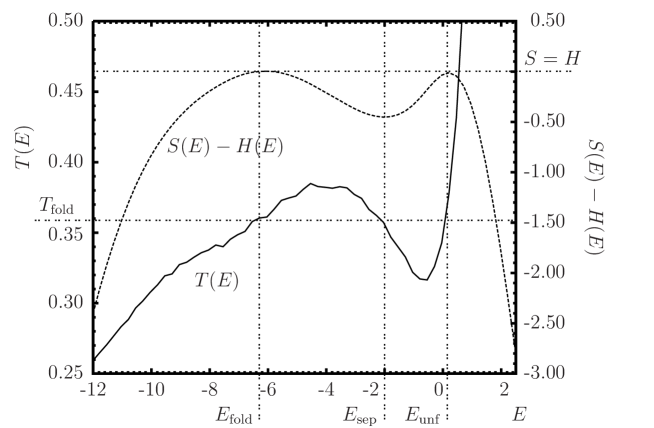
Figure 4: Folding transition as a phase-separation process for an exemplified 20mer in the AB model. In the transition region, the caloric temperature $T(E)$ of the protein decreases with increasing total energy. Folded and unfolded conformations coexist at the folding transition temperature, where $S(E)=H(E)$, corresponding to $T_{\rm fold}\approx 0.36$. The energetic transition region is bounded by the energies $E_{\rm fold}\approx-6.3$ and $E_{\rm unf}\approx 0.15$. Folding and unfolding regions are separated at $E_{\rm sep}\approx-2.0$.

However, the most striking feature in Fig. 4 is the qualitative change of the microcanonical temperature $T(E)$ in the transition region: Approaching from small energies (folded phase), the curve passes the folding temperature $T_{\rm fold}$ and follows the overheating branch. It then decreases with increasing energy (passing again $T_{\rm fold})$ before following the undercooling branch, crossing $T_{\rm fold}$ for the third time. In the unfolded phase, temperature and energy increase as expected. The unusual backbending of the caloric temperature curve within the transition region is not an artifact of the theory. It is a physical effect and has been confirmed in sodium cluster formation experiments [19], where a similar behavior was observed.

In Fig. 5, results from the canonical calculations (mean energy $\langle E\rangle$ and specific heat per monomer $c_{V}$) are shown as functions of the temperature. The specific heat exhibits a clear peak near $T=0.35$ which is close to the folding temperature $T_{\rm fold}$, as defined before in the microcanonical analysis. The loss of information by the canonical averaging process is apparent by comparing $\langle E\rangle$ and the inverse, non-unique mapping ${\cal F}^{-1}$ of microcanonical temperature and energy. The temperature decrease in the transition region from the folded to the unfolded structures is unseen in the plot of $\langle E\rangle$.

Figure 5: Comparison of canonical and microcanonical analysis for the folding transition: The fluctuations of energy as represented by the specific heat per monomer, $c_{V}(T)$, exhibit a sharp peak near $T\approx 0.35$. The canonical mean energy $\langle E\rangle(T)$ crosses over from the folded to the unfolded conformations. However, the canonical calculation averages out the overheating/undercooling branches and the backbending effect which are clearly signaled by the microcanonical analysis of the (inverse) mapping between temperature and energy. The microcanonically defined “folding temperature” $T_{\rm fold}$ is close to the peak temperature of the specific heat.

Eventually, as we had already mentioned when discussing the results shown in Fig. 3, there is also no unique canonical folding temperature signaled by peaks of fluctuating quantities; there are rather transition regions. Therefore, for small systems, the definition of transitions based on the canonical temperature is indeed little useful. Consequently, the microcanonical analysis is at least a powerful alternative for discussing conformational transitions of “small” systems. This also applies to molecular aggregation [13] and adsorption transitions [20], where similar phenomena can occur.

4 Conclusions

As we have exemplarily shown for the folding of proteins, conformational transitions of molecular systems can be well-described by analysis techniques known from statistical physics. However, the interpretation of these cooperative effects as thermodynamic phase transitions has noticeable limitations. This not only regards the impossibility to precisely identify definite transition points. It is even more fundamental to ask the question which of the typically used statistical ensembles provides the most comprehensive interpretation of finite-system structure formation processes. We have shown that the microcanonical analysis of folding thermodynamics is particularly advantageous, as, e.g., the remarkable temperature backbending effect is averaged out in the canonical ensembles, where the temperature is considered as an external control parameter which seems to be questionable for small systems [10, 11, 12, 13, 14].

I thank Wolfhard Janke for quite successful long-term collaboration. This work is partially supported by the DFG (German Science Foundation) under Grant Nos. JA 483/24-1/2/3. Support by a supercomputer time grant of the John von Neumann Institute for Computing (NIC), Forschungszentrum Jülich, is acknowledged.

References

- [1] M. Rubinstein and R.H. Colby, Polymer Physics, Oxford University Press, New York, 2003.
- [2] A. Maritan, C. Micheletti, A. Trovato, and J.R. Banavar, Nature 406 (2000) 287.
- [3] T. Vogel, T. Neuhaus, M. Bachmann, and W. Janke, Europhys. Lett. 85 (2009) 10003.
- [4] P.-G. de Gennes, Scaling Concepts in Polymer Physics, Cornell University Press, Ithaca, 1979.
- [5] P.J. Flory, Principles of Polymer Chemistry, Cornell University Press, Ithaca, 1953.
- [6] M. Bachmann and W. Janke, Lect. Notes Phys. 736 (2008) 203.
- [7] S. Schnabel, M. Bachmann, and W. Janke, Phys. Rev. Lett. 98 (2007) 048103; J. Chem. Phys. 126 (2007) 105102.
- [8] K.F. Lau and K.A. Dill, Macromolecules 22 (1989) 3986.
- [9] M. Bachmann and W. Janke, Phys. Rev. Lett. 91 (2003) 208105; J. Chem. Phys. 120 (2004) 6779.
- [10] D.H.E. Gross, Microcanonical Thermodynamics, World Scientific, Singapore, 2001.
- [11] S. Hilbert and J. Dunkel, Phys. Rev. E 74 (2006) 011120; J. Dunkel and S. Hilbert, Physica A 370 (2006) 390.
- [12] H. Behringer and M. Pleimling, Phys. Rev. E 74 (2006) 011108.
- [13] C. Junghans, M. Bachmann, and W. Janke, Phys. Rev. Lett. 97 (2006) 218103; J. Chem. Phys. 128 (2008) 085103; Europhys. Lett. in print (2009).
- [14] T. Chen, X. Lin, Y. Liu, and H. Liang, Phys. Rev. E 76 (2007) 046110.
- [15] F.H. Stillinger and T. Head-Gordon, Phys. Rev. E 52 (1995) 2872.
- [16] H.-P. Hsu, V. Mehra, and P. Grassberger, Phys. Rev. E 68 (2003) 037703.
- [17] M. Bachmann, H. Arkın, and W. Janke, Phys. Rev. E 71 (2005) 031906.
- [18] B.A. Berg and T. Neuhaus, Phys. Lett. B 267 (1991) 249; Phys. Rev. Lett. 68 (1992) 9.
- [19] M. Schmidt, R. Kusche, T. Hippler, J. Donges, W. Kronmüller, B. von Issendorff, and H. Haberland, Phys. Rev. Lett. 86 (2001) 1191.
- [20] M. Möddel, W. Janke, and M. Bachmann, preprint (2009).